Nonvanishing anisotropic magnetoresistance in Rashba two-dimensional electron systems with nonmagnetic disorders

Abstract

We study anisotropic magnetoresistance (AMR) in a spin-polarized two-dimensional electron gas with Rashba spin-orbit coupling and nonmagnetic disorder collision. We show that AMR exists, arising from the combined effect of in-plane magnetization, spin-orbit coupling, and nonmagnetic remote disorder scattering. Further, numerical evaluation demonstrates that the smoothness of the remote disorder can strongly affect AMR, and this AMR is sensitive to the electron density. Large magnitude of AMR ($\approx 24\%$) is obtained for low density system with strong spin-orbit splitting.

1 Introduction

Magnetotransport phenomena in ferromagnetic semiconductor, such as anisotropic magnetoresistance (AMR)[1, 2, 3, 4, 5, 6, 7, 8, 9, 10, 11, 12], have attracted significant attentions due to applications in the emerging field of spintronics [13, 14]. AMRs, including longitudinal and transverse AMRs, are the response of magnetoresistance to the relative angle between magnetization and current in magnetic materials. Both the longitudinal and transverse conductivities show the symmetric feature: $\sigma_{xx}(\bm{M}_{0})=\sigma_{xx}(-\bm{M}_{0})$ and $\sigma_{yx}(\bm{M}_{0})=\sigma_{yx}(-\bm{M}_{0})$, where the magnetization $\bm{M}_{0}$ is usually in the two-dimensional plane ($x$-$y$ plane). However, one should note that for ordinary charge Hall effect (including anomalous Hall effect [15]) the transverse conductivity obeys the antisymmetric relation, $\sigma_{yx}(\bm{M}_{0})=-\sigma_{yx}(-\bm{M}_{0})$. Here $\bm{M}_{0}$ is normal to the plane.

Experimentally, AMR has been extensively studied in diluted magnetic semiconductors recently. Rushforth et al. investigated the physical origin of the noncrystalline and crystalline components of AMR in diluted magnetic semiconductors [6]. Shin et al. explored the temperature dependence of AMR in ferromagnetic (Ga,Mn)As films [16]. A giant transverse AMR was also observed in this ternary ferromagnetic semiconductor (Ga,Mn)As [10, 9]. In contrast to the extensive experimental studies of AMR, the theoretical interpretation of AMR is relatively poor. The experimental analyses are usually based on a phenomenological treatment [2, 3]. The full Boltzmann theory simulations have been made to study the origin of the sources of AMR in $p$-type magnetic semiconductor [6, 8, 17]. Kato. et al. analyzed the intrinsic AMR in spin-polarized two-dimensional gas (2DEG) with Rashba spin-orbit coupling (SOC) [7]. They showed that AMR vanishes unless the relaxation time is spin-related. Recently, Trushin et al. studied AMR for Rashba or Dresselhaus spin-orbit splitting electron system with polarized magnetic impurities [18]. In the above theoretical studies, the microscopic mechanism of AMR is considered as due to the anisotropic carriers lifetime, arising from the combined effect of the SOC and the scattering by the polarized magnetic impurities. The spin-dependent scattering is the essential factor in AMR [12, 6, 8, 7, 18, 19]. In most studies, the nonmagnetic disorder potential is taken as $\delta$-form type. However in realistic heterostructure, the electron density is not large enough to screen the nonmagnetic impurities, where the interaction between electron and disorder is long-ranged. Hence, the effect of electron-impurity scattering on AMR is far from being understood, completely.

In this paper, we employ the kinetic equation approach to investigate AMR in two-dimensional electron system in the presence of Rashba-type spin-orbit interaction and in-plane magnetization. We show that the combined effect of SOC, in-plane magnetization, and nonmagnetic long-range impurity can lead to AMR. At the same time, numerical evaluation demonstrates the disorder-distance- and electron-density-related feature of AMR. The present study may provide another mechanism of AMR in spin-orbit interaction 2DEG with in-plane magnetization. The nonmagnetic wave-vector-dependent disorders, coupling to the SOC and magnetization, induces the magnetotransport anisotropy.

2 Theoretical approach

We consider a 2DEG confined in a [001]-grown III-V semiconductor heterostructure with Rashba SOC and a homogenous in-plane magnetization $\bm{M}_{0}$. The $x$ and $y$ axes are taken along [100] and [010] direction, respectively. Hence, the noninteracting one-particle Hamiltonian can be written as

$$\check{H}=\frac{k^{2}}{2m}+\alpha(\hat{z}\times\bm{\sigma})\cdot{\bm{k}}-M_{x}\sigma_{x}-M_{y}\sigma_{y}.$$ (1)

Here $m$ is the electron effective mass, $\bm{\sigma}\equiv(\sigma_{x},\sigma_{y},\sigma_{z})$ are the Pauli matrices, ${\bm{k}}\equiv(k\cos\theta_{\bm{k}},k\sin\theta_{\bm{k}})$ is the two-dimensional electron wave vector, $\alpha$ is the Rashba SOC parameter, and $\bm{M}\equiv(M_{x},M_{y})=M(\cos\xi,\sin\xi)=g\mu_{B}\bm{M}_{0}\equiv g\mu_{B}M_{0}(\cos\xi,\sin\xi)$ with ${g}$ as the effective $g$-factor, $\mu_{B}$ as the Bohr magneton, and $\xi$ as the angle between the magnetization $\bm{M}_{0}$ and [100]-axis.

The above Hamiltonian (1) can be diagonalized into $\hat{H}=U_{\bm{k}}^{\dagger}\check{H}U_{\bm{k}}={\rm diag}[\varepsilon_{1}(\bm{k}),\varepsilon_{2}(\bm{k})]$ in the helicity basis with the help of the following local unitary transformation

$$U_{\bm{k}}=\frac{1}{\sqrt{2}}\left(\begin{array}[]{cc}1&1\\ ie^{i\chi_{\bm{k}}}&-ie^{i\chi_{\bm{k}}}\\ \end{array}\right).$$ (2)

Here the energy dispersion $\varepsilon_{\mu}(\bm{k})=\frac{k^{2}}{2m}+(-1)^{\mu}\varepsilon_{\rm RM}(\bm{k})$ with $\varepsilon_{\rm RM}(\bm{k})=\sqrt{\alpha^{2}k^{2}+M^{2}+2\alpha kM\sin(\xi-\theta_{\bm{k}})}$, $\mu=1,2$ as the helix band index, and

$$\chi_{\bm{k}}=\tan^{-1}\frac{\alpha k\sin\theta_{\bm{k}}-M\cos\xi}{\alpha k\cos\theta_{\bm{k}}+M\sin\xi}.$$ (3)

Now we consider the quasi-two-dimensional system is driven by a weak dc electric field $\bm{E}$ along [100] direction. Obviously, in order to carry out the evaluation of the AMR, it is necessary to determine the matrix electron distribution function. The kinetic equation for the $2\times 2$ matrix distribution function $\rho(\bm{k})$ in the stationary linear response regime can be derived, where the elastic electron-impurity scattering is taken into account in the self-consistent Born approximation [20, 21, 22]. Following the procedure of these papers, the distribution function can be obtained as, $\rho(\bm{k})=\rho^{(0)}(\bm{k})+\rho^{(1)}(\bm{k})+\rho^{(2)}(\bm{k})$, with equilibrium distribution function $\rho^{(0)}(\bm{k})={\rm diag}\big{\{}n_{\rm F}[\varepsilon_{1}(\bm{k})],n_{\rm F}[\varepsilon_{2}(\bm{k})]\big{\}}$, and $n_{\rm F}(x)$ as the Fermi-Dirac function. Here $\rho^{(1)}(\bm{k})$ and $\rho^{(2)}(\bm{k})$ are collision-unrelated and collision-related matrix distribution functions in the first order of electric field, respectively. The collision-unrelated distribution function $\rho^{(1)}(\bm{k})$ is off-diagonal matrix with the elements given by

$$\rho^{(1)}_{12}(\bm{k})=\rho^{(1)}_{21}(\bm{k})=\frac{eE_{0}}{4\varepsilon_{\rm RM}}\frac{\partial\chi_{\bm{k}}}{\partial k_{x}}\big{\{}n_{\rm F}[\varepsilon_{1}(\bm{k})]-n_{\rm F}[\varepsilon_{2}(\bm{k})]\big{\}},$$ (4)

where $E_{0}$ is the strength of the electric field. This distribution function is associated with the interband transition between two spin-orbit-coupled bands, making no contribution to charge conductivity. However, it is important for spin Hall effect, which results in the collision-independent intrinsic spin Hall effect [23, 24, 22]. The collision-related distribution function $\rho^{(2)}(\bm{k})$ is determined by the coupled equations

$$eE_{0}\frac{\partial n_{\rm F}(\varepsilon_{\bm{k}\mu})}{\partial k_{x}} =\pi\sum_{\bm{q}\mu^{\prime}}|V(\bm{k}-\bm{q})|^{2}\Omega_{\mu\mu^{\prime}}$$

$$\times \left[\rho_{\mu\mu}^{(2)}(\bm{k})-\rho_{\mu^{\prime}\mu^{\prime}}^{(2)}(\bm{q})\right]\delta\big{[}\varepsilon_{\mu}(\bm{k})-\varepsilon_{\mu^{\prime}}(\bm{q})\big{]},$$ (5)

$$4\varepsilon_{\rm RM}(\bm{k}){\rm Re}\rho_{12}^{(2)}(\bm{k}) =\pi\sum_{\bm{q}\mu\mu^{\prime}}|V(\bm{k}-\bm{q})|^{2}\bar{\Omega}_{\mu\mu^{\prime}}$$

$$\times \left[\rho_{\mu\mu}^{(2)}(\bm{k})-\rho_{\mu^{\prime}\mu^{\prime}}^{(2)}(\bm{q})\right]\delta\big{[}\varepsilon_{\mu}(\bm{k})-\varepsilon_{\mu^{\prime}}(\bm{q})\big{]}.$$ (6)

Here $\Omega_{\mu\mu^{\prime}}=1+(-1)^{\mu+\mu^{\prime}}\cos(\chi_{\bm{k}}-\chi_{\bm{q}})$ and $\bar{\Omega}_{\mu\mu^{\prime}}=(-1)^{\mu^{\prime}}\sin(\chi_{\bm{k}}-\chi_{\bm{q}})$. $V(\bm{k}-\bm{q})$ is the nonmagnetic impurity scattering potential. ${\rm Re}\rho_{12}^{(2)}(\bm{k})$ represents the real part of the off-diagonal distribution function $\rho_{12}^{(2)}(\bm{k})$. One should note that here the weak scattering limit is assumed, where we restrict ourselves to the leading order of the impurity concentration. In this case, the imaginary part of the off-diagonal distribution function $\rho_{12}^{(2)}(\bm{k})$ can be ignored completely [20]. In the above kinetic equations, both the interband and the intraband transitions are considered.

In order to study AMR, it is necessary to evaluate the drift velocity. In spin basis, the two in-plane matrix velocity operators read

$$\check{v}_{x}=\left(\begin{array}[]{cc}\frac{k_{x}}{m}&i\alpha\\ -i\alpha&\frac{k_{x}}{m}\\ \end{array}\right),$$ (7)

$$\check{v}_{y}=\left(\begin{array}[]{cc}\frac{k_{y}}{m}&\alpha\\ \alpha&\frac{k_{y}}{m}\\ \end{array}\right).$$ (8)

It is clear that the velocity operators in spin basis are independent of the magnetization. Moreover, the expressions of the velocity operators are the same as the ones of semiconductor heterostructure with Rashba spin-orbit interaction in the absence of magnetization. However, in the helicity basis, the single-particle operators of velocity $\hat{v}_{i}=U_{\bm{k}}^{\dagger}\check{v}_{i}U_{\bm{k}}$ ($i=x,y$), rely on the magnetization through the energy spectrum and the angle $\chi_{\bm{k}}$, and are given by

$$\hat{v}_{x}=\left(\begin{array}[]{cc}\frac{\partial\varepsilon_{1}(\bm{k})}{\partial k_{x}}&i\alpha\sin\chi_{\bm{k}}\\ -i\alpha\sin\chi_{\bm{k}}&\frac{\partial\varepsilon_{2}(\bm{k})}{\partial k_{x}}\\ \end{array}\right),$$ (9)

$$\hat{v}_{y}=\left(\begin{array}[]{cc}\frac{\partial\varepsilon_{1}(\bm{k})}{\partial k_{y}}&-i\alpha\cos\chi_{\bm{k}}\\ i\alpha\cos\chi_{\bm{k}}&\frac{\partial\varepsilon_{2}(\bm{k})}{\partial k_{y}}\\ \end{array}\right).$$ (10)

One find that the off-diagonal elements of in-plane velocity operators are also nonvanishing in helicity basis. The corresponding macroscopical drift velocities are obtained by taking the statistical average over them, $v_{i}=\frac{1}{N}\sum_{\bm{k}}{\rm Tr}[\rho(\bm{k})\hat{v}_{i}]$, and expressed as

$$v_{i}=\frac{1}{N}\sum_{\bm{k}\mu}\frac{\partial\varepsilon_{\mu}(\bm{k})}{\partial k_{i}}\rho_{\mu\mu}^{(2)}(\bm{k}).$$ (11)

Here $N$ is the electron density. It can be seen that the average velocities only depend on the diagonal element of velocity operators. One should emphasize that in clean limit approximation, the imaginary part of the off-diagonal element of collision-related distribution function vanishes. Hence, the drift velocities only relate to the diagonal elements of velocity operators and the diagonal elements of distribution function. And the expressions of average velocities become the same as the usual form of two band system without interband coupling. We only need Eq. (5) to determine the diagonal elements of distribution function. The real part of off-diagonal elements, ${\rm Re}\rho_{12}^{(2)}(\bm{k})$, is essential for calculation of spin Hall effect [21, 22] and anomalous Hall effect [20]. The longitudinal and transverse conductivities are defined by $\sigma_{xx}=Nev_{x}/E_{0}$ and $\sigma_{yx}=Nev_{y}/E_{0}$, respectively.

For AMR, one can find that the longitudinal and transverse conductivities obey the symmetric relations: $\sigma_{xx}(\bm{M}_{0})=\sigma_{xx}(-\bm{M}_{0})$ and $\sigma_{yx}(\bm{M}_{0})=\sigma_{yx}(-\bm{M}_{0})$. We can understand these properties as follows: The eigenenergy $\varepsilon_{\mu}(\bm{M}_{0},\bm{k})$ and angle $\chi_{\bm{k}}(\bm{M}_{0})$ satisfy $\varepsilon_{\mu}(-\bm{M}_{0},-\bm{k})=\varepsilon_{\mu}(\bm{M}_{0},\bm{k})$ and $\chi_{-\bm{k}}(-\bm{M}_{0})=\pi+\chi_{\bm{k}}(\bm{M}_{0})$. Therefore distribution function satisfies $\rho_{\mu\mu}^{(2)}(-\bm{M}_{0},-\bm{k})=-\rho_{\mu\mu}^{(2)}(\bm{M}_{0},\bm{k})$. Note that for brevity, the argument $\bm{M}_{0}$ for eigenenergy, distribution function and so on, is dropped elsewhere. When $\bm{M}_{0}\rightarrow-\bm{M}_{0}$, we make transformation $\bm{k}\rightarrow-\bm{k}$ in Eq. (11). This transformation will not change the total integral, hence the conductivities satisfy the symmetric property. This property is in vivid contrast to the one of anomalous Hall effect, where the transverse conductivity obeys the antisymmetric relation. Now we remark these relations from the point of view of the time reversal symmetry. For AMR, the conductivities are related to the diagonal elements of distribution function, which are proportional to a momentum-dependent effective transport relaxation time $\tau_{\rm tr}$ (see footnote). However, the anomalous Hall conductivity relies on the off-diagonal elements. The off-diagonal elements do not depend on this effective transport relaxation time, directly, and the disorder plays only an intermediate role [20]. Under time reversal, for AMR, $\sigma_{xx}(-\bm{M}_{0},-\tau_{\rm tr})=-\sigma_{xx}(\bm{M}_{0},\tau_{\rm tr})$ and $\sigma_{yx}(-\bm{M}_{0},-\tau_{\rm tr})=-\sigma_{yx}(\bm{M}_{0},\tau_{\rm tr})$. By considering the relations between the conductivities and the effective relaxation time, one can obtain the symmetric feature. While for anomalous Hall conductivity $\sigma_{yx}(-\bm{M}_{0})=-\sigma_{yx}(\bm{M}_{0})$ under time reversal, and the antisymmetric relation is obtained directly.

3 Numerical results

We numerically investigate the combined effect of Rashba SOC, magnetization, and long-range nonmagnetic electron-impurity scattering on the AMR in InAs/InSb heterostructure. The long-range electron-impurity collision is considered as due to remote nonmagnetic charged impurities separated at a distance $s$ from the interface. The potential takes the form $V({q})=U({q})/\kappa({q})$ with $|U({q})|^{2}=n_{i}\left(\frac{e^{2}}{2\epsilon_{0}\kappa q}\right)^{2}e^{-2qs}I(q)^{2}$ [25, 26]. Here $I(q)$ is the form factor and $\kappa({q})$ is the factor related to the Coulomb screening, the expressions of which can be found in Ref. [26]. $n_{i}$ is the density of nonmagnetic remote impurity. In the calculation the electron effective mass is taken as $m=0.04m_{\rm e}$ with $m_{\rm e}$ as the free electron mass. The dielectric constant of InAs $\kappa=15.15$. In the numerical analysis, we have assumed that $\varepsilon_{\rm F}>M$, i.e. both the minority and the majority bands are occupied, with $\varepsilon_{\rm F}$ as the Fermi energy.

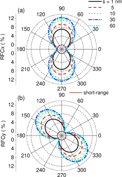
Figure 1: The relative fractional change in the longitudinal (a) and transverse (b) conductivities as functions of the angle $\xi$ between magnetization in the plane and [100]-axis for various remote impurity distances. The thin wine lines are obtained for $\delta$-form short-range electron-disorder collision. The electron density $N=1.0\times 10^{11}\,{\rm cm}^{-2}$. Rashba constant $\alpha=3.0\times 10^{-11}\,{\rm eVm}$ and the magnetization $M=2\,{\rm meV}$.

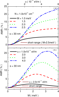
Figure 2: AMR is shown as functions of spin-orbit interaction parameter for various magnetizations (a) and as functions of magnetization for various Rashba coupling parameters (b) at fixed distance $s=30\,{\rm nm}$. Here the electron concentration $N=1.0\times 10^{11}{\rm cm}^{-2}$. The thin wine lines indicate the corresponding AMR for short-range electron-impurity scattering.

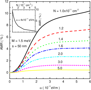
Figure 3: Dependencies of AMR on SOC constant $\alpha$ for different electron densities. The magnetization $M=1.5\,{\rm meV}$ and the remote impurity distance $s=50\,{\rm nm}$. The inset shows AMR as functions of electron density when Rashba spin-orbit splitting $\alpha=4.0\times 10^{-11}\,{\rm eVm}$.

We first consider the relative fractional changes in the conductivity (RFC), which are defined by

$${\rm RFCx} = \frac{\Delta\sigma_{xx}}{\sigma_{av}}-\left(\frac{\Delta\sigma_{xx}}{\sigma_{av}}\right)_{\rm min},$$ (12)

$${\rm RFCy} = \frac{\Delta\sigma_{yx}}{\sigma_{av}}-\left(\frac{\Delta\sigma_{yx}}{\sigma_{av}}\right)_{\rm min},$$ (13)

where $\Delta\sigma_{xx}=\sigma_{xx}-\sigma_{av}$, $\Delta\sigma_{yx}=\sigma_{yx}-\sigma_{av}$, and $\sigma_{av}$ is the average value of the longitudinal conductivity as the magnetization is rotated through $360^{\circ}$ with respect to [100]-axis. The subscript “min” means the corresponding minimum value of the fractional change. It is seen that RFC is independent of impurity density.

In Fig. 1, the relative fractional changes in the longitudinal and transverse conductivities are shown as functions of the angle between magnetization in the plane and [100]-axis for this nonmagnetic remote disorder. The corresponding thin wine solid line is obtained for $\delta$ shape short-range electron-disorder collision, $V(q)=V_{0}$, independent of momentum. It is clear that the longitudinal conductivity shows the strong anisotropy for magnetization aligned along various direction when the nonmagnetic disorder is long-ranged. However, the anisotropy completely vanishes for short-range electron-impurity scattering, in agreement with the previous studies [7, 18]. The degree of this anisotropy depends strongly on the smoothness of the remote disorder. With the rise of the impurity distance, the degree of the anisotropy first enhances, and then drops when the distance is large enough. In Fig. 1 (b), it is seen that the transverse conductivity also indicates the anisotropy for various direction of magnetization. The remote disorders can affect the degree of the anisotropy of transverse conductivity, similar to the longitudinal conductivity. It is also found that, when the nonmagnetic disorder becomes short-ranged, the anisotropy of transverse conductivity also vanishes completely. This confirms that the combined effect of Rashba SOC, in-plane magnetization, and nonmagnetic remote disorder could lead to AMR. Our numerical evaluation shows that these longitudinal and transverse AMRs are consistent with the standard phenomenology due to symmetry arguments [6, 18]: ${\Delta\sigma_{xx}}/{\sigma_{av}}=C_{I}\cos 2\xi$, ${\Delta\sigma_{yx}}/{\sigma_{av}}=C_{I}\sin 2\xi$. Here $C_{I}$ is a dimensionless constant and is sometimes called noncrystalline coefficient in literatures. One note that crystalline AMR coefficient vanishes in this case, which is a special property of the Rashba model. It is not valid for systems with other SOC, such as Dresselhaus SOC [18].

Now we limit ourselves to AMRs defined as the relative change between longitudinal resistivities for magnetization along and normal to the current direction. We take the current direction along [100]-axis. In this case, it is found that the transverse conductivity vanishes. Hence, AMR is given by

$${\rm AMR}=\frac{\rho_{xx}^{\parallel}-\rho_{xx}^{\perp}}{(\rho_{xx}^{\parallel}+\rho_{xx}^{\perp})/2}=2\frac{\sigma_{xx}^{\perp}-\sigma_{xx}^{\parallel}}{\sigma_{xx}^{\parallel}+\sigma_{xx}^{\perp}}.$$ (14)

Here $\sigma_{xx}^{\parallel}$ and $\sigma_{xx}^{\perp}$ are the corresponding longitudinal conductivities for $\bm{M}\parallel\bm{J}$ and $\bm{M}\perp\bm{J}$ with $\bm{J}$ as the current density. Also one find that this definition of AMR is disorder-density-independent.

In Fig. 2(a), we plot AMRs as functions of spin-orbit interaction constant for various magnetizations at fixed impurity distance $s=30\,{\rm nm}$. It is seen that the magnitude of magnetization can affect AMR strongly. A large AMR ($\sim 24\%$) can be observed for Rashba coupling parameter up to $6\times 10^{11}\,{\rm eVm}$ at $M=2.5\,{\rm meV}$. With the increment of Rashba SOC coefficient, AMR ascends and may saturate at strong coupling. We also evaluate the dependencies of AMR on the magnitude of magnetization for various SOC constants in Fig. 2(b). With the rise of magnetization, AMR first increases, and then decreases. However, AMR is always positive. The strength of the spin-orbit interaction can affect both the value and the position of maximum AMR. For short-range nonmagnetic impurity, AMR vanishes completely.

In order to investigate the density-related feature of AMR, in Fig. 3, AMRs are calculated for various electron density for fixed magnetization and disorder distance. It is clear that AMR is very sensitive to the electron concentration. With the increasing density, AMR, arising from the electric remote scattering in SOC semiconductor with in-plane magnetization, drops quickly. For $N=5.0\times 10^{11}\,{\rm cm}^{-2}$ at large coupling constant, ${\rm AMR}\sim 0.45\%$. It is small but still measurable experimentally [6]. The inset shows the dependence of AMR on electron density for $\alpha=4\times 10^{-11}\,{\rm eVm}$. This implies vanishing AMR in the limit of $k_{+}(\theta_{\bm{k}})\approx k_{-}(\theta_{\bm{k}})$ with $k_{\pm}(\theta_{\bm{k}})$ as the two angle-dependent Fermi wave vectors.

We now make some comments on the experiments to confirm the present results. Since we deals with AMR arising from nonmagnetic disorder, the nonmagnetic $n$-type InAs-based heterojunction can be well satisfied. The in-plane magnetization may be induced by an in-plane magnetic field. The magnitude of magnetic field corresponds to a magnetization $M=1\,{\rm meV}$ is $2.16\,\rm T$ (in InAs-based heterojunction, the effective $g$-factor $g=8$ [27]). The Rashba SOC constant can be tuned by controlling the gate voltage. The usual Hall setup is well satisfied to measure this AMR. We note that Papadakis et al. reported the observation of AMR of two-dimensional holes in nonmagnetic GaAs [28]. Our present study may provide a possible interpretation of that novel phenomenon. However, careful theoretical investigation should be made for $p$-type semiconductor systems.

4 Conclusion

In summary, AMR for two-dimensional electron systems with a Rashba-type spin-orbit splitting and an in-plane magnetization is investigated for nonmagnetic impurity collision. It is found that the combined effect of SOC, in-plane magnetization, and electric remote disorder leads to AMR. The disorder distance can strongly affect the degree of anisotropy of longitudinal and transverse conductivity. The strong density-related character of AMR is also demonstrated.

- [1] \NameThomson W. \REVIEWProc. R. Soc.81857546.
- [2] \NameSmit J. \REVIEWPhysica171951612.
- [3] \NameMcGuire T., Potter R. \REVIEWIEEE Trans. Magn.1119751018.
- [4] \NameJaoul O., Campbell I. A. Fert A. \REVIEWJ. Magn. & Magn. Mater.5197723.
- [5] \NameBaxter D. V., Ruzmetov D., Scherschligt J., Sasaki Y., Liu X., Furdyna J. K. Mielke C. H. \REVIEWPhys. Rev. B652002212407.
- [6] \NameRushforth A. W., Výborný K., King C. S., Edmonds K. W., Campion R. P., Foxon C. T., Wunderlich J., Irvine A. C., Vašek P., Novák V., Olejniḱ K., Sinova J., Jungwirth T. Gallagher B. L. \REVIEWPhys. Rev. Lett.992007147207.
- [7] \NameKato T., Ishikawa Y., Itoh H. Inoue J. I. \REVIEWPhys. Rev. B772008233404.
- [8] \NameRushforth A. W., Výborný K., King C. S., Edmonds K. W., Campion R. P., Foxon C. T., Wunderlich J., Irvine A. C., Novák V., Olejník K., Kovalev A. A., Sinova J., Jungwirth T. Gallagher B. L. \REVIEWJ. Magn. & Magn. Mater.32120091001.
- [9] \NameTang H. X., Kawakami R. K., Awschalom D. D. Roukes M. L. \REVIEWPhys. Rev. Lett.902003107201.
- [10] \NamePappert K., Hümpfner S., Wenisch J., Brunner K., Gould C., Schmidt G. Molenkamp L. W. \REVIEWAppl. Phys. Lett.902007062109.
- [11] \NameLim W. L., Liu W., K. Dziatkowski Z. G., Shen S., Furdyna J. K. Dobrowolska M. \REVIEWJ. Appl. Phys.99200608D505.
- [12] \NameKovalev A. A., Tserkovnyak Y., Výborný K. Sinova J. \REVIEWPhys. Rev. B792009195129.
- [13] \NameWolf S. A., Awschalom D. D., Buhrman R. A., Daughton J. M., von Molnar S., Roukes M. L., Chtchelkanova A. Y. Treger D. M. \REVIEWScience29420011488.
- [14] \NameJungwirth T., Sinova J., Mašek J., Kučera J. MacDonald A. H. \REVIEWRev. Mod. Phys.782006809.
- [15] \NameSinitsyn N. A. \REVIEWJ. Phys.: Condens. Matter202008023201.
- [16] \NameShin D. Y., Chung S. J., Lee S., Liu X. Furdyna J. K. \REVIEWPhys. Rev. B762007035327.
- [17] \NameVýborný K., Kučera J., Sinova J., Rushforth A. W., Gallagher B. L. Jungwirth T. \REVIEWPhys. Rev. B802009165204.
- [18] \NameTrushin M., Výborný K., Moraczewski P., Kovalev A. A., Schliemann J. Jungwirth T. \REVIEWPhys. Rev. B802009134405.
- [19] \NameVýborný K., Kovalev A. A., Sinova J. Jungwirth T. \REVIEWPhys. Rev. B792009045427.
- [20] \NameLiu S. Y. Lei X. L. \REVIEWPhys. Rev. B722005195329.
- [21] \NameLiu S. Y. Lei X. L. \REVIEWPhys. Rev. B722005155314.
- [22] \NameLin Q., Liu S. Y. Lei X. L. \REVIEWAppl. Phys. Lett.882006122105.
- [23] \NameMurakami S., Nagaosa N. Zhang S.-C. \REVIEWScience30120031348.
- [24] \NameSinova J., Culcer D., Niu Q., Sinitsyn N., Jungwirth T. MacDonald A. \REVIEWPhys. Rev. Lett.922004126603.
- [25] \NameStern F. Howard W. E. \REVIEWPhys. Rev.1631967816.
- [26] \NameLei X. L., Birman J. L. Ting C. S. \REVIEWJ. Appl. Phys.5819852270.
- [27] \NameSmith III T. P. Fang F. F. \REVIEWPhys. Rev. B3519877729.
- [28] \NamePapadakis S. J., Poortere E. P. D. Shayegan M. \REVIEWPhys. Rev. Lett.8420005592.