Cosmological test of gravity with polarizations of stochastic gravitational waves around 0.1-1 Hz

Abstract

In general relativity, a gravitational wave has two polarization modes (tensor mode), but it could have additional polarizations (scalar and vector modes) in the early stage of the universe, where the general relativity may not strictly hold and/or the effect of higher-dimensional gravity may become significant. In this paper, we discuss how to detect extra-polarization modes of stochastic gravitational wave background (GWB), and study the separability of each polarization using future space-based detectors such as BBO and DECIGO. We specifically consider two plausible setups of the spacecraft constellations consisting of two and four clusters, and estimate the sensitivity to each polarization mode of GWBs. We find that a separate detection of each polarization mode is rather sensitive to the geometric configuration and distance between clusters and that the clusters should be, in general, separated by an appropriate distance. This seriously degrades the signal sensitivity, however, for suitable conditions, space-based detector can separately detect scalar, vector and tensor modes of GWBs with energy density as low as $h_{0}^{2}\Omega_{\rm gw}\sim 10^{-15}$.

I Introduction

Incoherent superposition of gravitational waves produced by many unresolved sources or diffuse sources forms a stochastic background of gravitational waves (GWs), whose statistical properties contain valuable information about the high-energy astrophysical phenomena and the cosmic structure formation. In particular, with the gravitational wave backgrounds (GWBs), we can directly probe the very early Universe beyond the last-scattering surface of the cosmic microwave background.

Various mechanisms or scenarios have been proposed for generation of cosmological GWBs in the early universe, via the inflation Grishchuk (1974); Rubakov et al. (1982); Abbott and Wise (1984); Allen (1988), cosmological phase transition Kosowsky et al. (1992); Kamionkowski et al. (1994); Grojean and Servant (2007); Kahniashvili et al. (2008), and reheating of the Universe Khlebnikov and Tkachev (1997); Easther and Lim (2006); Dufaux et al. (2007); Garcia-Bellido and Figueroa (2007); J. Garcia-Bellido and Sastre (2008) and etc.. An important aspect of those scenarios is that general relativity (GR) may not strictly hold in the high-energy regime of the universe, and the gravitational waves do not necessarily satisfy the transverse and traceless conditions. This implies that the number of polarization modes of a GW is more than that of tensor modes (i.e., two polarization modes called plus and cross modes), and it can have six modes at most in the four-dimensional spacetime, including scalar and vector modes bib (a); Eardley et al. (1973). In modified gravity theories such as Brans-Dicke theory Brans and Dicke (1961); bib (b) and $f(R)$ gravity bib (c); Capozziello et al. (2009), such additional polarizations appear (For more rigorous treatment of the polarizations with the Newman-Penrose formalism, see Alves et al. (2009); bib (d)). Further, there are several attractive scenarios that we live in a three-dimensional brane embedded in a higher-dimensional spacetime, such as the Kaluza-Klein theory and the Dvali-Gabadadze-Porrati (DGP) braneworld model Dvali et al. (2000). In those models, even the tensor modes satisfying the transverse and traceless conditions can have extra polarization degrees, which propagate in the extra-dimensional bulk spacetime. The effects of higher-dimensional gravity are expected to be significant at high-energy scales, and thus the cosmological GWBs generated during such a stage may have additional polarization modes, which can be viewed as the mixture of scalar and vector polarizations in the projected three-dimensional space. In these respects, the polarization modes of GWBs provide additional information about the physics of the early universe, and thus a search for extra-polarization modes is indispensable as a cosmological test of GR. Note also that the polarization of GWB from astrophysical origin can also be useful as a test of strong gravity associated with astrophysical phenomena.

Currently, there is no observational evidence for GWBs, and the constraints on the extra-polarization modes of GWBs are almost nonexistent . However, the observations of cosmic microwave background anisotropies are currently consistent with the adiabatic density perturbations plus negligible contribution of tensor GWB bib (e) and no significant contributions of scalar and vector GWBs are expected. Further, a search for stochastic GWBs by LIGO bib (f) has given an upper limit on the energy density of GWBs around $\sim 100$Hz, $h^{2}\Omega_{\rm{gw}}\lesssim 3.6\times 10^{-6}$, where $\Omega_{\rm{gw}}$ is the energy density per logarithmic frequency bin normalized by the critical density of the Universe, and the present Hubble parameter normalized by $H_{0}=100\,h_{0}\,\rm{km\,sec^{-1}\,Mpc^{-1}}$. This null detection is applied to the constraints on the GWBs of extra-polarization modes with correction by a factor of a few, depending on the response of the GW detectors to each polarization mode.

In this paper, we investigate how well we can separately detect and measure the polarizations of a GWB using space-based GW detectors. Previously, we have studied the detection and separation of polarization modes of GWB using a network of ground-based laser interferometers (for a detection of GWB using the pulsar timing arrays, see Ref.  Lee et al. (2008)). With the correlation signals obtained from more than three advanced detectors, we found that scalar, vector and tensor modes of GWBs can be separately detected around the frequencies $f\sim 100$Hz, and the sensitivity to each polarization mode can reach $h_{0}^{2}\Omega_{\rm{gw}}=10^{-9}\sim 10^{-8}$. Extending the previous analysis to those using space-based interferometers, we discuss a direct detection of extra-polarization modes of low-frequency GWBs at $f=0.1\sim 1$Hz.

Currently, several space missions to detect GWs have been proposed. Among these, DECI-hertz interferometer Gravitational-wave Observatory (DECIGO) Seto et al. (2001); bib (g) and Big-Bang Observer (BBO) bib (h) (also see Cutler and Holz (2009) for updated information) will aim at detecting cosmological GWBs generated during the inflationary epoch as the primary target. These orbit the Sun with a period of one sidereal year, and constitute several clusters, each of which consists of three spacecrafts exchanging laser beams with the others, as shown in Fig. 1. DECIGO plans to have the arm-length $10^{3}\,{\rm{km}}$, equipped with Fabry-Perot cavity in each arm, while BBO will adopt the transponder type with arm-length $10^{4}\,{\rm{km}}$. The crucial difference between space- and ground-based detectors is that practical design as well as precise orbital configurations for space interferometers are still under debate, and there are a number of options for the detector configuration. Hence, in this paper, we will examine several plausible setups and discuss under what conditions we can separately measure the scalar, vector and tensor polarizations of GWB.

This paper is organized as follows. In Sec. II, for notational convenience, we first present the definitions of GW polarizations. Then, we discuss a methodology to separately detect the polarization modes, based on the previous analysis using the ground-based interferometers. In Sec. III, we investigate the separability of the polarization modes of the GWB in specific configurations of space-based detectors, and calculate the detector sensitivities to each polarization mode, especially focusing on DECIGO. Sec. IV presents discussion on the low-frequency cutoff due to the presence of astronomical confusion noise, and the sensitivity to polarizations in the BBO case. Finally, the paper is summarized in Sec. V.

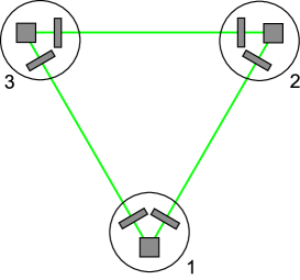
Figure 1: A cluster of DECIGO.

II Formulation

II.1 GW polarizations and detector response

We start by briefly reviewing the basic concepts of data analysis of stochastic GWB search. First consider the spacetime metric generated by a stochastic GWB in the observed three-dimensional space. At a position $\vec{\mathbf{X}}$ and time $t$, it is expressed as

$$\mathbf{h}(t,\vec{\mathbf{X}}) = \sum_{p}\int_{S^{2}}d\hat{\mathbf{\Omega}}\int_{-\infty}^{\infty}df\,$$ (1)

$$\times\tilde{h}_{p}(f,\hat{\mathbf{\Omega}})\,e^{2\pi if(t-\hat{\mathbf{\Omega}}\cdot\vec{\mathbf{X}}/c)}\,\mathbf{e}_{p}(\hat{\mathbf{\Omega}})\>,$$

where $c$ is the speed of light bib (i), $f$ is frequency of a GW, and $\hat{\mathbf{\Omega}}$ is a unit vector pointed at the GW propagating direction. The amplitude $\tilde{h}_{p}(f,\hat{\mathbf{\Omega}})$ represents the Fourier transform of the GW amplitude for each polarization mode, and the quantity $\mathbf{e}_{p}$ is the polarization tensor. Including the extra-polarization degrees of scalar and vector modes, we have six polarization modes in three-dimensional space; $p=+,\times,b,\ell,x,$ and $y$, which are called plus, cross, breathing, longitudinal, vector-x, and vector-y modes, respectively. Using the orthonormal vectors, $\hat{\mathbf{m}}$ and $\hat{\mathbf{n}}$, perpendicular to the direction vector $\hat{\mathbf{\Omega}}$ (as shown in Fig. 2), the polarization tensors are defined by Eardley et al. (1973); bib (a)

$$\mathbf{e}_{+} = \hat{\mathbf{m}}\otimes\hat{\mathbf{m}}-\hat{\mathbf{n}}\otimes\hat{\mathbf{n}}\;,$$

$$\mathbf{e}_{\times} = \hat{\mathbf{m}}\otimes\hat{\mathbf{n}}+\hat{\mathbf{n}}\otimes\hat{\mathbf{m}}\;,$$

$$\mathbf{e}_{b} = \hat{\mathbf{m}}\otimes\hat{\mathbf{m}}+\hat{\mathbf{n}}\otimes\hat{\mathbf{n}}\;,$$

$$\mathbf{e}_{\ell} = \sqrt{2}\,\hat{\mathbf{\Omega}}\otimes\hat{\mathbf{\Omega}}\;,$$

$$\mathbf{e}_{x} = \hat{\mathbf{m}}\otimes\hat{\mathbf{\Omega}}+\hat{\mathbf{\Omega}}\otimes\hat{\mathbf{m}}\;,$$

$$\mathbf{e}_{y} = \hat{\mathbf{n}}\otimes\hat{\mathbf{\Omega}}+\hat{\mathbf{\Omega}}\otimes\hat{\mathbf{n}}\;.$$

Each polarization mode is orthogonal to one another and is normalized so that $e_{ij}^{p}e^{ij}_{p^{\prime}}=2\delta_{pp^{\prime}}$ for $p,p^{\prime}=+,\times,b,\ell,x,$ and $y$. Note that the breathing and longitudinal modes do not satisfy the traceless condition, in contrast to the ordinary plus and cross polarization modes in GR. For the universe with extra-dimensions, the number of polarization modes generally can be more than six, but in the projected three-dimensional space, GW can be viewed as a mixture of scalar, vector and tensor modes mentioned above.

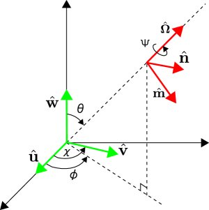
Figure 2: Coordinate systems.

Next consider the response of the GW detector. The laser interferometers measure the time variation of the spacetime metric as one-dimensional time-series data. In a space-based interferometer, the gravitational-wave signal is obtained by differentiating two link signals in Fig.1 (three interferometer signals is obtained about a cluster.). Denoting the signal strain measured by the interferometer $I$ (whose position is located at $\vec{\mathbf{X}}$) by $h_{I}(t)$, the strain amplitude of GW is expressed as

$$h_{I}(t,\vec{\mathbf{X}}) = \mathbf{D}_{I}:\mathbf{h}(t,\vec{\mathbf{X}})$$ (2)

$$= \sum_{p}\int_{S^{2}}d\hat{\mathbf{\Omega}}\int_{-\infty}^{\infty}df\,$$

$$\times\,\tilde{h}_{p}(f,\hat{\mathbf{\Omega}})\,e^{2\pi if(t-\hat{\mathbf{\Omega}}\cdot\vec{\mathbf{X}}/c)}F_{I}^{p}(f,\hat{\mathbf{\Omega}})\>,$$

where the quantity $\mathbf{D}_{I}$ is the detector tensor, and the $F_{I}^{p}$ is the angular response function for each polarization mode. They are respectively given by

$$F^{p}_{I}(\hat{\mathbf{\Omega}}) \equiv \mathbf{D}_{I}:\mathbf{e}_{p}(\hat{\mathbf{\Omega}})\;,$$ (3)

$$\mathbf{D}_{I} \equiv \frac{1}{2}\left[\hat{\mathbf{u}}\otimes\hat{\mathbf{u}}-\hat{\mathbf{v}}\otimes\hat{\mathbf{v}}\right]\>,$$ (4)

with the unit vectors $\hat{\mathbf{u}}$ and $\hat{\mathbf{v}}$ being directed to each detector arm. The expression of Eq. (4) is valid when the arm length of the detector, $L$, is much smaller than the wavelength of observed GWs, $\lambda_{\rm{g}}$, i.e., $L\ll\lambda_{\rm g}$. For DECIGO, the observable frequency range is around $f\sim 1\,\rm{Hz}$, which corresponds to $\lambda_{\rm{g}}=3\times 10^{5}\,\rm{km}$. Thus, with the arm length $L=10^{3}\,\rm{km}$, the so-called low frequency approximation is fully satisfied.

II.2 Cross-correlation analysis

Throughout the paper, we assume that stochastic GWB is (i) isotropic, (ii) stationary, (iii) Gaussian, and (iv) has no intrinsic correlation between polarization modes (If this is not the case, see Allen and Ottewill (1997); Cornish (2001a); Kudoh and Taruya (2005); Taruya and Kudoh (2005); Kudoh et al. (2006); Taruya (2006); Thrane et al. (2009) and Drasco and Flanagan (2003); Himemoto et al. (2007); Seto (2008) for discussions on the detection of GWBs in the presence of anisotropies and non-Gaussianity, respectively.). Adopting these assumptions, all the statistical properties of the GWB are characterized by the power spectral density:

$$\langle\tilde{h}_{p}^{\ast}(f,\hat{\Omega})\tilde{h}_{p^{\prime}}(f^{\prime},\hat{\Omega^{\prime}})\rangle = \delta(f-f^{\prime})\frac{1}{4\pi}\delta^{2}(\hat{\Omega},\hat{\Omega^{\prime}})\delta_{pp^{\prime}}$$ (5)

$$\quad\quad\times\,\frac{1}{2}S_{h}^{p}(|f|)\;,$$

where $\delta^{2}(\hat{\Omega},\hat{\Omega^{\prime}})\equiv\delta(\phi-\phi^{\prime})\delta(\cos\theta-\cos\theta^{\prime})$, and $\langle\cdots\rangle$ denotes ensemble average. The function $S_{h}^{p}(f)$ is the one-sided power spectral density for each polarization mode.

Conventionally, the amplitude of GWB for each polarization is also characterized by an energy density per logarithmic frequency bin, normalized by the critical energy density of the Universe:

$$\Omega_{\rm{gw}}^{p}(f)\equiv\frac{1}{\rho_{c}}\frac{d\rho_{\rm{gw}}^{p}}{d\ln f}=\left(\frac{2\pi^{2}}{3H_{0}^{2}}\right)f^{3}S_{h}^{p}(f)\>,$$ (6)

where $\rho_{c}=3H_{0}^{2}/8\pi G$ and $H_{0}$ is the Hubble constant. In the second equality, we used the relation between $\Omega_{\rm{gw}}(f)$ and $S_{h}(f)$ given by Maggiore (2000); Allen and Romano (1999). Then, we define the GWB energy density in tensor, vector, and scalar polarization modes as

$$\Omega_{\rm{gw}}^{T} \equiv \Omega_{\rm{gw}}^{+}+\Omega_{\rm{gw}}^{\times}\;,$$

$$\Omega_{\rm{gw}}^{V} \equiv \Omega_{\rm{gw}}^{x}+\Omega_{\rm{gw}}^{y}\;,$$

$$\Omega_{\rm{gw}}^{S} \equiv \Omega_{\rm{gw}}^{b}+\Omega_{\rm{gw}}^{\ell}=\Omega_{\rm{gw}}^{b}(1+\kappa)\;,$$

The subscripts $T$, $V$, and $S$ stand for tensor, vector, and scalar, respectively. Hereafter, we assume $\Omega_{\rm{gw}}^{+}=\Omega_{\rm{gw}}^{\times}$ for the tensor mode and $\Omega_{\rm{gw}}^{x}=\Omega_{\rm{gw}}^{y}$ for the vector mode. This assumption is valid for a stochastic GWB generated in most of cosmological scenarios bib (j). For the scalar mode, we introduce a model-dependent new parameter, $\kappa(f)\equiv\Omega_{\rm{gw}}^{\ell}(f)/\Omega_{\rm{gw}}^{b}(f)$.

In order to discriminate a stochastic GWB from random detector noise, one needs to cross-correlate between detector signals Christensen (1992); Flanagan (1993); Allen and Romano (1999). Let us consider the outputs of a detector, $s(t)=h(t)+n(t)$, where $h(t)$ and $n(t)$ are the GW signal and the noise of a detector. In general, the amplitude of GWB is thought to be much smaller than that of detector noise. Cross-correlation signal $Y$ between two detectors is given by

$$Y \equiv \int_{-T_{\rm{obs}}/2}^{T_{\rm{obs}}/2}dt\int_{-T_{\rm{obs}}/2}^{T_{\rm{obs}}/2}dt^{\prime}\,s_{I}(t)s_{J}(t^{\prime})Q(t-t^{\prime})\;,$$ (7)

$$\approx \int_{-\infty}^{\infty}df\int_{-\infty}^{\infty}df^{\prime}\delta_{T}(f-f^{\prime})\tilde{s}_{I}^{*}(f)\tilde{s}_{J}(f^{\prime})\tilde{Q}(f^{\prime}),$$

where $T_{\rm{obs}}$ is observation time, $\tilde{s}_{I}(f)$, $\tilde{s}_{J}(f)$ and $\tilde{Q}(f)$ are the Fourier transforms of $s_{I}(t)$, $s_{J}(t)$ and $Q(t-t^{\prime})$, respectively. $Q(t-t^{\prime})$ is a filter function, which will be later adjusted to maximize the signal-to-noise ratio (SNR) of correlation signal. The function $\delta_{T}(f)$ is defined by

$$\delta_{T}(f)\equiv\int_{-T_{\rm{obs}}/2}^{T_{\rm{obs}}/2}dt\,e^{-2\pi ift}=\frac{\sin(\pi fT_{\rm{obs}})}{\pi f}\>.$$

Taking the ensemble average over the expression (7), and substituting Eqs. (5) and (6) into this, we obtain a GW signal in a correlation analysis between $I$-th and $J$-th detectors,

$$\mu \equiv \langle Y\rangle$$ (8)

$$= \int_{-\infty}^{\infty}df\int_{-\infty}^{\infty}df^{\prime}\delta_{T}(f-f^{\prime})\langle\tilde{h}_{I}^{*}(f)\tilde{h}_{J}(f^{\prime})\rangle\tilde{Q}(f^{\prime})\>.$$

$$= \frac{3H_{0}^{2}}{20\pi^{2}}T_{\rm{obs}}\,\sin^{2}\chi\int_{-\infty}^{\infty}df|f|^{-3}\tilde{Q}(f)$$

$$\times \biggl{[}\Omega_{\rm{gw}}^{T}(f)\gamma^{T}_{IJ}(f)+\Omega_{\rm{gw}}^{V}(f)\gamma^{V}_{IJ}(f)$$

$$+\xi(f)\,\Omega_{\rm{gw}}^{S}(f)\gamma^{S}_{IJ}(f)\biggr{]}\;,$$

$$\xi(f) \equiv \frac{1}{3}\left(\frac{1+2\kappa(f)}{1+\kappa(f)}\right)\;.$$

The parameter $\xi$ takes the value in the range $1/3\leq\xi\leq 2/3$ and characterizes the ratio of the energy in the longitudinal mode to the breathing mode. The sensitivity to the GWB can be governed by the so-called overlap reduction functions Christensen (1992); Flanagan (1993); Allen and Romano (1999), which represents how much of the correlation of the GW signal between detectors can be preserved. The overlap reduction function for each polarization is defined by Nishizawa et al. (2009)

$$\gamma_{IJ}^{M}(f) \equiv \frac{1}{\sin^{2}\chi}\int_{S^{2}}\frac{d\hat{\Omega}}{4\pi}\,e^{2\pi if\hat{\Omega}\cdot\Delta\vec{X}/c}\,{\cal{R}}_{IJ}^{M}\;,$$ (9)

$${\cal{R}}_{IJ}^{T}(\hat{\mathbf{\Omega}}) \equiv \frac{5}{2}\,(F_{I}^{+}F_{J}^{+}+F_{I}^{\times}F_{J}^{\times})\;,$$

$${\cal{R}}_{IJ}^{V}(\hat{\mathbf{\Omega}}) \equiv \frac{5}{2}\,(F_{I}^{x}F_{J}^{x}+F_{I}^{y}F_{J}^{y})\;,$$

$${\cal{R}}_{IJ}^{S}(\hat{\mathbf{\Omega}}) \equiv \frac{15}{1+2\kappa}\,(F_{I}^{b}F_{J}^{b}+\kappa F_{I}^{\ell}F_{J}^{\ell})\;,$$

which are normalized to unity in the limit $f\to 0$. The subscript $M$ denotes $M=T,V,S$, and the quantity $\Delta\vec{\mathbf{X}}$ is the separation vector defined by $\Delta\vec{\mathbf{X}}\equiv\vec{\mathbf{X}}_{I}-\vec{\mathbf{X}}_{J}$. Note that the prefactor, $\sin^{2}\chi=1-(\hat{\mathbf{u}}\cdot\hat{\mathbf{v}})^{2}$, in Eq. (9) comes from the non-orthogonal detector arms. For an equilateral triangle configuration of the spacecraft constellation in Fig. 1, we have $\sin^{2}\chi=3/4$.

In Eq. (9), the angular integral is analytically performed prior to specifying the detector location and orientation Nishizawa et al. (2009). The result is expressed as

$$\gamma_{IJ}^{M}(f) = \frac{1}{\sin^{2}\chi}\biggl{[}\rho_{1}^{M}(\alpha)D_{I}^{ij}D^{J}_{ij}+\rho_{2}^{M}(\alpha)D_{I,\,k}^{i}D_{J}^{kj}\hat{d}_{i}\hat{d}_{j}$$ (10)

$$+\rho_{3}^{M}(\alpha)D_{I}^{ij}D_{J}^{k\ell}\hat{d}_{i}\hat{d}_{j}\hat{d}_{k}\hat{d}_{\ell}\biggr{]}\;,$$

with unit vector $\hat{d}_{i}$ defined by $\hat{d}_{i}\equiv\Delta\vec{X}/|\Delta\vec{X}|$. The summation is taken over each component of the subscripts $i,j,k,\ell$. In the above, frequency dependence of the overlap reduction function is incorporated into the coefficients, $\rho^{M}_{1}$, $\rho^{M}_{2}$, and $\rho^{M}_{3}$, which sensitively depend on each polarization mode. We have

$$\left(\begin{array}[]{c}\rho_{1}^{T}\\ \rho_{2}^{T}\\ \rho_{3}^{T}\end{array}\right)=\frac{1}{14}\left(\begin{array}[]{ccc}28&-40&2\\ 0&120&-20\\ 0&0&35\end{array}\right)\left(\begin{array}[]{c}j_{0}\\ j_{2}\\ j_{4}\end{array}\right)\;,$$

for tensor mode,

$$\left(\begin{array}[]{c}\rho_{1}^{V}\\ \rho_{2}^{V}\\ \rho_{3}^{V}\end{array}\right)=\frac{2}{7}\left(\begin{array}[]{ccc}7&5&-2\\ 0&-15&20\\ 0&0&-35\end{array}\right)\left(\begin{array}[]{c}j_{0}\\ j_{2}\\ j_{4}\end{array}\right)\;,$$

for vector mode, and

$$\left(\begin{array}[]{c}\rho_{1}^{S}\\ \rho_{2}^{S}\\ \rho_{3}^{S}\end{array}\right)=\frac{1}{7}\left(\begin{array}[]{ccc}14&20&6\\ 0&-60&-60\\ 0&0&105\end{array}\right)\left(\begin{array}[]{c}j_{0}\\ j_{2}\\ j_{4}\end{array}\right)\;.$$

for scalar mode. Here, $j_{n}(\alpha)$ is the spherical Bessel function with its argument given by

$$\alpha(f)\equiv\frac{2\pi fD}{c}\;,\quad\quad D\equiv|\Delta\vec{X}|\;.$$ (11)

These expressions are very useful to obtain a simple expression for the overlap reduction function in specific detector configurations below.

Let us now consider the noise part in the cross correlation analysis. As long as the intrinsic noise correlation between two detectors is absent, the ensemble average of cross correlation quantity $Y$ in Eq. (7) is dominated by the GW signals. This is true even in the weak signal limit, $h\ll n$. However, the variance of $Y$ is dominated by the detector noises. We obtain

$$\sigma^{2} \equiv \langle Y^{2}\rangle-\langle Y\rangle^{2}$$ (12)

$$\approx \langle Y^{2}\rangle$$

$$\approx \int_{-\infty}^{\infty}df\int_{-\infty}^{\infty}df^{\prime}\,\tilde{Q}(f)\tilde{Q}^{\ast}(f^{\prime})\,$$

$$\times\langle\tilde{n}^{\ast}_{I}(f)\tilde{n}_{I}(f^{\prime})\rangle\,\langle\tilde{n}_{J}(f)\tilde{n}^{\ast}_{J}(f^{\prime})\rangle$$

$$\approx \frac{T_{\rm{obs}}}{4}\int_{-\infty}^{\infty}df\,P_{I}(|f|)P_{J}(|f|)\,|\tilde{Q}(f)|^{2}\>,$$

where the one-sided power spectrum density of the detector noise, $P_{I}(f)$, is defined by

$$\langle\tilde{n}^{\ast}_{I}(f)\tilde{n}_{J}(f^{\prime})\rangle\equiv\frac{1}{2}\delta(f-f^{\prime})\delta_{IJ}P_{I}(|f|)\;.$$

For DECIGO, the analytical fit of the noise power spectrum is obtained for a single interferometer. Assuming that the detector noise is idealistically limited by the sum of quantum noises, i.e., shot noise, $P^{\rm{shot}}$, and radiation-pressure (acceleration) noise, $P^{\rm{acc}}$, we have bib (k):

$$P(f) = P^{\rm{acc}}(f)+P^{\rm{shot}}(f)$$

$$P^{\rm{acc}}(f) = 6.31\times 10^{-51}\biggl{(}\frac{f}{1\rm{Hz}}\biggr{)}^{-4}\;\rm{Hz}^{-1}\;,$$

$$P^{\rm{shot}}(f) = 1.88\times 10^{-48}+5.88\times 10^{-50}\biggl{(}\frac{f}{1\rm{Hz}}\biggr{)}^{2}\;\rm{Hz}^{-1}\;.$$

In Fig. 3, the noise power spectrum of DECIGO is plotted as the strain amplitude, $S_{h}^{1/2}$.

Figure 3: DECIGO noise curve.

From Eqs. (8) and (12), the SNR in the correlation analysis between two detectors is simply given by ${\rm{SNR}}=\mu/\sigma$. In the absence of extra-polarization degrees (i.e., only the tensor modes exit), two-detector correlation is sufficient to detect GWB, and the optimal choice of the filter function $\tilde{Q}(f)$ is easy to derive Allen and Romano (1999). On the other hand, in the presence of multiple polarization modes, we need more than three detectors in order to separately detect each polarization mode. The optimal SNR combining multiple detectors is not simply given by the sum of $\mu/\sigma$, and thus the choice of filter function is rather non-trivial. We will discuss this issue in the next section.

II.3 Signal-to-noise ratio

In principle, three polarization modes, i.e., scalar, vector and tensor, can be separately detected by linearly combining more than three independent correlation signals. In our previous paper Nishizawa et al. (2009), we considered the situation that only the three correlation signals are available. We then presented the formula for optimal SNR. Here, we consider the optimal SNR combining arbitrarily large number, $N_{\rm{pair}}$, of correlation signals. Such a generalized formula has been derived for the cases with two polarizations (i.e., circularly polarized and un-polarized modes of tensor GWs) by Seto and Taruya Seto and Taruya (2008). Based on this, in Appendix B, the extension of the formula to the three-polarization case is presented. Combining $N_{\rm{pair}}$ correlation signals, the resultant optimal SNR for separately detecting scalar, vector and tensor GWBs becomes (see Eq. (LABEL:eq47))

$${\rm{SNR}}^{M}=\frac{9H_{0}^{2}}{40\pi^{2}}\biggl{[}2\int_{0}^{\infty}df\,\frac{(\Omega_{\rm{gw}}^{M}(f))^{2}\det\mathbf{F}(f)}{f^{6}{\cal{F}}_{M}(f)}\biggr{]}^{1/2},\;\;$$ (13)

$$\mathbf{F}(f)=\left(\begin{array}[]{ccc}F_{TT}&F_{TV}&F_{TS}\\ F_{TV}&F_{VV}&F_{VS}\\ F_{TS}&F_{VS}&F_{SS}\end{array}\right)\;,\quad\quad\quad\quad\quad\;\;$$ (17)

$$F_{MM^{\prime}}(f)=\sum_{i}\int_{0}^{T_{\rm{obs}}}dt\,\frac{\gamma_{i}^{M}(t,f)\gamma_{i}^{M^{\prime}}(t,f)}{{\cal{N}}_{i}(f)}\;,\quad\;\;$$ (18)

where $M$ and $M^{\prime}$ denote polarization modes, $M,M^{\prime}=T,V,S$. The quantity ${\cal{F}}_{M}$ is the determinant of the sub-matrix, which is constructed by removing the $M$’s elements from $\mathbf{F}$. The subscript $i$ indicates a pair of detectors (e.g., $i=(I,J)$ for pair of $I$- and $J$-th detectors), and ${\cal{N}}_{i}(f)$ is defined as, say, ${\cal{N}}_{12}(f)\equiv P_{1}(f)P_{2}(f)$. In what follows, for simplicity, we consider the case that all interferometers have the same noise spectrum, i.e., $P_{I}(f)=P(f)$.

The expression (13) is a rather general formula for optimal SNR in the sense that the stationary configuration of GW detectors is not strictly assumed. The configuration of space-based interferometers gradually changes in time due to the orbital motion of the spacecrafts. In the formula (13), the effect of such gradual change is incorporated into the explicit time dependence of the overlap reduction function, which will be important later in Sec. III.2. Note that for stationary detector configuration, the time integral in Eq. (18) simply reduces to the factor $T_{\rm{obs}}$, which gives rise to the well-known result that $SNR\propto T_{\rm{obs}}^{1/2}$. Further, if we consider the combination of three detectors ($N_{\rm{pair}}=3$), the above SNR can be reduced to Eq. (53) in Ref. Nishizawa et al. (2009) except for the prefactor $\sin^{2}\chi=3/4$ or (124) in this paper.

The expression (13) is one of the most important results of this paper. Provided the location and orientation of GW detectors, the SNR is quantitatively evaluated. Before doing so, it is important to note that a separate detection of three polarization modes is possible only when the quantity $\det\mathbf{F}$ becomes non-vanishing. As we explain in detail below, this implies that the configuration of space-based detectors must satisfy both conditions:

(i)

The detectors have to be separated by at least the distance of a typical wavelength of the observed GWs, e.g., $3\times 10^{5}\,{\rm{km}}$ for a GW with frequency $f=1\,{\rm{Hz}}$.

(ii)

Detector pairs are not geometrically degenerate, e.g., three detectors located at the vertices of a non-equilateral triangle.

If one of the two conditions fails, the SNR is expected to be significantly degraded.

For intuitive explanation of the above two conditions, let us consider the three-detector (three correlation-signal) case Nishizawa et al. (2009) (This does not lose generality because one can verify that SNR with an arbitrary number of detectors can be reduced to weighted sum of SNR with three-detector subset.). In the case, the condition $\det\mathbf{F}\neq 0$ corresponds to $\det\mathbf{\Pi}\neq 0$ where

$$\mathbf{\Pi}(f)\equiv\left(\begin{array}[]{ccc}\gamma^{T}_{12}&\gamma^{V}_{12}&\gamma^{S}_{12}\\ \gamma^{T}_{23}&\gamma^{V}_{23}&\gamma^{S}_{23}\\ \gamma^{T}_{31}&\gamma^{V}_{31}&\gamma^{S}_{31}\end{array}\right)\;.$$

The condition (i) comes from nondegeneracy of the components in a column of $\mathbf{\Pi}$, e.g. $\gamma^{T}_{12}\neq\gamma^{V}_{12}\neq\gamma^{S}_{12}$. As we will see explicitly in Sec. III, for a closer detector pair ($\alpha\rightarrow 0$), there is no difference in the overlap reduction functions for each polarization mode, since the spherical Bessel functions, $j_{2}$ and $j_{4}$ vanish. On the other hand, for a detector pair with $\alpha\sim 1$, $j_{2}$ and $j_{4}$ are of the same order as $j_{0}$ and result in differences between the overlap reduction functions. The condition (ii) comes from nondegeneracy of the components in a row of $\mathbf{\Pi}$, e.g. $\gamma^{T}_{12}\neq\gamma^{T}_{23}\neq\gamma^{T}_{31}$. This condition implies that a non-colinear configuration of three detectors is preferred.

III Sensitivity to polarization modes

We are in a position to discuss how well one can separately detect scalar, vector and tensor GWBs. In this section, we specifically consider the two setups of detector configuration, and estimate the detectability for each polarization mode. First, we consider the four-cluster configuration with coplanar orbits (case I). This is the prototypical configuration proposed at an early phase of the conceptual design of DECIGO bib (g). We then move to a discussion of two-cluster configuration, in which the orbits of two clusters are slightly inclined in relation to one another (case II). In the calculations below, the energy spectrum of GWBs $\Omega_{\rm{gw}}^{M}(f)$ is assumed to be a flat spectrum, i.e., $\Omega_{\rm{gw}}^{M}=$const. In computing SNR below, we do not consider the single-cluster correlation. This is because correlation signals from a single cluster are not sensitive enough to GWB at low frequencies, as discussed in Appendix A.

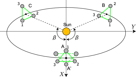
Figure 4: Case I — Four clusters, A, A’, B, and C, sharing the coplanar orbit, whose radius is $1\,{\rm{AU}}$.

III.1 Case I: four clusters

III.1.1 Configuration

Let us consider the detector configuration consisting of four clusters shown in Fig. 4. Each cluster is inclined by 60 degrees from the orbital plane in order to close the orbit. The guiding center of each cluster, i.e., the center-of-mass of three spacecrafts, follows a circular orbit around the Sun, with the radius $R_{0}=1\,{\rm{AU}}\approx 1.5\times 10^{8}\,{\rm{km}}$ and orbital period of one year. In the coordinate system $(X,Y,Z)$ shown in Fig. 4, the position of the guiding center is given by

$$\vec{X}(t)=(R_{0}\cos\phi(t),\,R_{0}\sin\phi(t),\,0\,)\;,$$

where the phase of the orbit is $\phi(t)=\omega_{\rm{orbit}}t=2\pi(t/{1\rm{yr}})$ for the clusters A and A’. The phases of the clusters B and C are relatively shifted to $\beta$ and $-\beta$ from that of the clusters A and A’, respectively. Thus, the distances between the clusters, $D\equiv|\Delta\vec{\mathbf{X}}|$, become $D_{\rm{AB}}(\beta)=D_{\rm{AC}}(\beta)=2R_{0}|\sin(\beta/2)|$ for the AB and AC link, and $D_{\rm{BC}}(\beta)=2R_{0}|\sin\beta|$ for the BC link.

In each cluster, the position of the spacecraft relative to the guiding center is given by

$$\vec{\mathbf{x}}_{i}(t) = \mathbf{R}_{Z}\bigl{[}-\phi(t)\bigr{]}\,\mathbf{R}_{Y}\bigl{[}-\theta\bigr{]}\,\mathbf{R}_{Z}\bigl{[}\phi(t)\bigr{]}\,\vec{\mathbf{x}}_{i,0}\;,$$ (19)

$$\vec{\mathbf{x}}_{i,0} = \frac{L}{\sqrt{3}}\times(\,\cos\sigma_{i},\,\sin\sigma_{i},\,0\,)\;.$$ (20)

with $\theta=\pi/3$. The matrices $\mathbf{R}_{Y}$ and $\mathbf{R}_{Z}$ are the rotation matrices around $Y$ and $Z$ axes, respectively. The angle $\sigma_{i}$ represents the orientation angle of the bisector of two arms of each interferometer. Let the angle of the interferometer 1 be $\sigma_{1}=\sigma_{0}$. The orientations of interferometer 2 and 3 in a cluster are given by $\sigma_{2}=\sigma_{0}+2\pi/3$ and $\sigma_{3}=\sigma_{0}+4\pi/3$, respectively.

In the setup mentioned above, the angles $\beta$ and $\sigma_{0}$ are apparently regarded as the free parameters. However, in an optimal combination of detector signals, several examinations reveal that the resultant SNR is turns out to be insensitive to any choice of $\sigma_{0}$. We thus set $\sigma_{0}=0$, and treat the separation angle $\beta$ as the only free parameter. For simplicity of the calculation below, the separation of the detectors between different clusters is approximated as the distance between the guiding centers of each cluster. This treatment is validated as long as we are interested in the low-frequency GWs satisfying $\lambda_{g}\gg L$. Then, the detector configuration can become stationary, and no explicit time-dependence appears at the overlap reduction functions in Eq. (13).

III.1.2 Overlap reduction functions

For each detector link of four-cluster configuration, the overlap reduction function given by Eq. (10) is reduced to a rather compact expression. For correlation signals of AB, AC, BC links, the overlap reduction functions are respectively written as

$$\gamma^{M}_{AB}(f,\beta,\sigma_{A},\sigma_{B};\alpha_{AB})=\frac{1}{16}\quad\quad\quad\quad\quad\quad\quad\quad\quad$$

$$\times\biggl{[}\Theta_{1}^{M}(\alpha_{AB},\beta/2)\,\cos[2(\sigma_{A}-\sigma_{B})]\quad\quad\quad\quad$$

$$-\Theta_{2}^{M}(\alpha_{AB},\beta/2)\,\sin[2(\sigma_{A}-\sigma_{B})]\quad\quad\quad\quad$$

$$+\Theta_{3}^{M}(\alpha_{AB},\beta/2)\,\cos[2\beta-2(\sigma_{A}+\sigma_{B})]\biggr{]}\;,\;\;$$ (21)

$$\gamma^{M}_{AC}(f,\beta,\sigma_{A},\sigma_{C};\alpha_{AC})=\gamma^{M}_{AB}(f,-\beta,\sigma_{A},\sigma_{C};\alpha_{AB})\;,$$

and

$$\gamma^{M}_{BC}(f,\beta,\sigma_{B},\sigma_{C};\alpha_{BC})=\frac{1}{16}\quad\quad\quad\quad\quad\quad\quad\quad\quad$$

$$\times\biggl{[}\Theta_{1}^{M}(\alpha_{BC},\beta)\,\cos[2(\sigma_{B}-\sigma_{C})]\quad\quad\quad\quad\quad$$

$$+\Theta_{2}^{M}(\alpha_{BC},\beta)\,\sin[2(\sigma_{B}-\sigma_{C})]\quad\quad\quad\quad\quad$$

$$+\Theta_{3}^{M}(\alpha_{BC},\beta)\,\cos[2(\sigma_{B}+\sigma_{C})]\biggr{]}\;.\quad\quad\quad\;\;\;$$ (23)

Note that the overlap reduction function for $AA^{\prime}$ link becomes $\gamma^{M}_{AA^{\prime}}=1$, because of the mirror symmetry. As for A’B and A’C links, the overlap reduction functions are identical to those for AB and AC links. Here, the function $\Theta^{M}_{i}(\alpha,\beta)$ is defined by

$$\Theta_{1,2}^{M}(\alpha,\beta)\equiv J_{M}(\alpha)\,U_{1,2}(\beta)\;,$$

$$\left(\begin{array}[]{c}\Theta_{3}^{T}(\alpha,\beta)\\ \Theta_{3}^{V}(\alpha,\beta)\\ \Theta_{3}^{S}(\alpha,\beta)\end{array}\right) \equiv -9\left[\left(\begin{array}[]{c}J_{T}(\alpha)\\ J_{V}(\alpha)\\ J_{S}(\alpha)\end{array}\right)\sin^{4}\beta\right.$$ (30)

$$+ \frac{5}{14}\left(\begin{array}[]{c}-8j_{2}(\alpha)-j_{4}(\alpha)\\ 4j_{2}(\alpha)+4j_{4}(\alpha)\\ 8j_{2}(\alpha)-6j_{4}(\alpha)\end{array}\right)\sin^{2}\beta$$ (34)

$$+ \left.\frac{5}{9}\left(\begin{array}[]{c}j_{4}(\alpha)\\ -4j_{4}(\alpha)\\ 6j_{4}(\alpha)\end{array}\right)\right]\;.$$ (38)

$$U_{1}(\beta) \equiv \sin^{4}\beta+8\cos^{6}\beta(1+\cos^{2}\beta)\;,$$ (39)

$$U_{2}(\beta) \equiv 2\bigl{(}1+\cos^{2}\beta\bigr{)}\bigl{(}1+\cos^{2}\beta+2\cos^{4}\beta\bigr{)}\,\sin 2\beta\;,$$

$$J_{T}(\alpha) \equiv j_{0}(\alpha)+\frac{5}{7}j_{2}(\alpha)+\frac{3}{112}j_{4}(\alpha)\;,$$ (41)

$$J_{V}(\alpha) \equiv j_{0}(\alpha)-\frac{5}{14}j_{2}(\alpha)-\frac{3}{28}j_{4}(\alpha)\;,$$ (42)

$$J_{S}(\alpha) \equiv j_{0}(\alpha)-\frac{5}{7}j_{2}(\alpha)+\frac{9}{56}j_{4}(\alpha)\;.$$ (43)

The subscript $M$ stands for the polarization mode, $T,V,S$. The angles $\sigma_{A}$, $\sigma_{B}$, and $\sigma_{C}$ are the orientation of the interferometer in the clusters A, B, and C, respectively. $\alpha_{AB}$, $\alpha_{AC}$, and $\alpha_{BC}$ imply the dimensionless frequency $\alpha$ defined in Eq. (11) for AB, AC, and BC links. Note that from the expressions (21)-(23), the overlap reduction functions are invariant under the transformation $\sigma\to\sigma+n\pi/2$ except for an overall sign. This is due to the quadrupole nature of GWs.

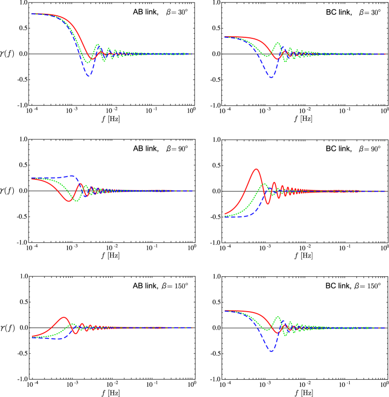
Figure 5: Overlap reduction functions of the correlation between interferometers in cluster A and B (left panels) and cluster B and C (right panels) in the case I. The orientations of the interferometers are selected as $\sigma_{A}=\sigma_{B}=\sigma_{C}=0$. Solid (red), dotted (green), and dashed (blue) curves correspond to the tensor, vector, and scalar modes, respectively.

In the four-cluster configuration, the detector separation $D$ is typically of the order of 1 AU. This means that the overlap reduction function starts to oscillate, and rapidly decay above the characteristic frequency, $f_{c}\equiv c/(2D)\sim 10^{-3}\,\rm{Hz}$. Examples of the overlap reduction function for each polarization mode are shown in Fig. 5, where the parameters of detector configuration are selected as $\sigma_{A}=\sigma_{B}=\sigma_{C}=0$, and the results for $\beta=30^{\circ},90^{\circ}$, and $150^{\circ}$ are plotted from top to bottom panels. At the frequency $f\sim 0.1$Hz, the amplitudes of overlap reduction function are significantly dropped, but they show different oscillatory behaviors for each polarization mode. The latter property is essential for separately detecting the scalar, vector and tensor GWBs. Note that the distance between BC link becomes identical for top and bottom panels, and the overlap reduction functions for each polarization mode coincide with each other.

In the present setup, the condition for separate detection of each polarization mode can be understood more precisely from Eqs. (21) - (23). Consider the close detectors with $\alpha\ll 1$ and $\beta<1$. The spherical Bessel functions are approximated as

$$j_{n}(\alpha)\approx\frac{\alpha^{n}}{(2n+1)!!}\;.$$

Further, we obtain $U_{1}(\beta)=16+{\cal{O}}(\beta^{2})$ and $U_{2}(\beta)=32\beta+{\cal{O}}(\beta^{3})$. Then, terms including $j_{2}$ and $j_{4}$ become negligible, and we have

$$\gamma_{AB}^{M} \approx j_{0}(\alpha)[1+{\cal{O}}(\beta)]\cos\bigl{[}2(\sigma_{A}-\sigma_{B})\bigr{]}\;,$$

$$\gamma_{BC}^{M} \approx j_{0}(\alpha)[1+{\cal{O}}(\beta)]\cos\bigl{[}2(\sigma_{B}-\sigma_{C})\bigr{]}\;.$$

Clearly, the overlap reduction functions for all polarization modes become degenerate, and reduce to an identical form in the limit $\beta\to 0$. Therefore, the $j_{2}$ and $j_{4}$ terms play a crucial role in breaking this degeneracy. These terms become comparable to the $j_{0}$ term only when $\alpha\gtrsim 1$, leading to the condition $D>\lambda_{g}$. Hence, widely separated detectors are essential for separately measuring each polarization mode of GWB. However, this generally conflicts with the optimal detection of GWBs. The resultant sensitivity to each polarization mode is thus significantly reduced, as shown below.

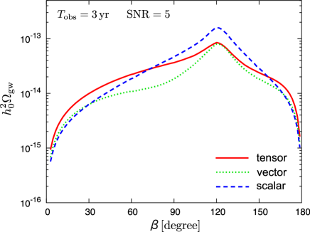
Figure 6: Detectable $h_{0}^{2}\Omega_{\rm{gw}}$ ($\xi h_{0}^{2}\Omega_{\rm{gw}}$ for the scalar mode) after the mode separation in the case I.

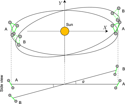
Figure 7: Case II — Two clusters, A and B, whose radius of the orbits is $1\,{\rm{AU}}$. The orbital plane of the cluster B is tilted by the angle $\psi$.

III.1.3 Results

The optimal SNR for four-cluster configuration is calculated with, in total, 54 correlation signals (AA’, AB, AC, A’B, A’C, BC $\times 9\;{\rm{links}}=54$). Setting the observation time and detection threshold to $T_{\rm{obs}}=3\,{\rm{yr}}$ and ${\rm{SNR}}=5$, we estimate minimum detectable amplitude $h_{0}^{2}\Omega_{\rm{gw}}$ ($\xi h_{0}^{2}\Omega_{\rm{gw}}$ for the scalar mode).

In Fig. 6, the resultant amplitude is plotted as function of angle $\beta$. At $\beta\sim 120^{\circ}$, the sensitivity degrades due to the symmetry of the detector configuration. In other words, the clusters, A, B, and C, are located at the apexes of an equilateral triangle, and some of the correlation signals are degenerated. As $\beta$ approaches $0^{\circ}$ and $180^{\circ}$, the detector sensitivity reaches nearly maximum, because the clusters A and B (or C), and B and C are close to the colocated configuration. In practice, to keep a better angular resolution to point GW sources, two of four clusters have to be located far from the star-like clusters Holz and Hughes (2005); Cutler and Holz (2009). Thus, the optimal choice of the parameter $\beta$ may be around $\beta\sim 60^{\circ}$, which gives the detectable amplitude for each polarization mode as

$$h_{0}^{2}\Omega_{\rm{gw}}^{T}=2.2\times 10^{-14},$$

$$h_{0}^{2}\Omega_{\rm{gw}}^{V}=1.1\times 10^{-14},$$

$$\xi h_{0}^{2}\Omega_{\rm{gw}}^{S}=1.9\times 10^{-14}.$$

These results are compared with the optimal detection of GWB without mode separation. For two clusters that are colocated and coaligned like clusters A and A’, the sensitivity reaches $h_{0}^{2}\Omega_{\rm{gw}}|_{0}=7.1\times 10^{-17}$. Thus, for a separate detection of polarization modes, the sensitivity to GWB is significantly degraded by more than two orders of magnitude.

III.2 Case II: two clusters

III.2.1 Configuration

For better measurement of each polarization of GWB, we consider an alternative setup shown in Fig. 7 originally proposed by Ref. Seto (2007) in order to detect a circularly polarized component of tensor GWB. In this setup, the orbital configuration of the one cluster is the same as cluster A in case I, while the orbital plane of the other cluster B is slightly tilted by the angle $\psi$ around the $Y$ axis. The position of each spacecraft in cluster A is described by Eqs. (19) and (20), with specific choice of the parameters, $\theta=\pi/3$, $\sigma_{1}=0$, $\sigma_{2}=2\pi/3$, and $\sigma_{3}=4\pi/3$. The orbit of the guiding center of the cluster B, and the relative positions of the spacecrafts are respectively given by

$$\vec{X}_{B}(t) = \mathbf{R}_{Y}\bigl{[}-\psi\bigr{]}\,\vec{X}_{A}(t)\;,$$

$$\vec{\mathbf{x}}_{B}(t) = \mathbf{R}_{Y}\bigl{[}-\psi\bigr{]}\,\vec{\mathbf{x}}_{A}(t)\;.$$

Note that, seen at a certain moment $t$, the intercluster correlation signals (the overlap reductions) between cluster A and B are highly degenerate due to the geometrical degeneracy in the interferometer location (e.g. $\gamma^{T}_{A1B1}\neq\gamma^{T}_{A1B2}\neq\gamma^{T}_{A1B3}$). So, the differences between the overlap reduction functions are of the order of ${\cal{O}}(L^{2}/D^{2})$. However, the degeneracy can be broken by utilizing the orbital motion of the clusters. The advantage of this configuration is that the distance between the clusters gradually changes with time, and the correlation signals measured at the different times can be regarded as that of a different detector pair with different location and separation. As a result of closer detector separation, the sensitivity to each polarization mode can become even better compared to the four-cluster configuration.

As long as we consider the low-frequency GWs, the detector separation is approximately described by $D(\psi,\phi)=2R_{0}\left|\sin(\psi/2)\,\cos\phi\right|$. Since $\phi$ assigns a time to an overlap reduction function, the inclination angle $\psi$ is the only free parameter. In what follows, instead of $\psi$, we use the maximum separation of clusters, $D_{\rm{max}}=2R_{0}|\sin(\psi/2)|$, to characterize the results.

III.2.2 Overlap reduction function

Compared to the case I, the analytical expressions of overlap reduction functions for two-cluster configuration become much more complicated, but can be obtained from Eq. (10). For a cross-correlation signal of AB links, the overlap reduction functions are

$$\gamma^{M}(f,\phi,\psi,\sigma_{A},\sigma_{B};\alpha) = \frac{1}{16}\biggl{[}\Theta_{1}^{M}(\alpha,\phi,\psi)\,\cos[2(\sigma_{A}+\sigma_{B})]+\Theta_{2}^{M}(\alpha,\phi,\psi)\,\sin[2(\sigma_{A}+\sigma_{B})$$

$$\quad+\Theta_{3}^{M}(\alpha,\phi,\psi)\,\cos[2(\sigma_{A}-\sigma_{B})]+\Theta_{4}^{M}(\alpha,\phi,\psi)\,\sin[2(\sigma_{A}-\sigma_{B})]\biggr{]}\;,$$

where

$$\left(\begin{array}[]{c}\Theta_{1,2}^{T}\\ \Theta_{1,2}^{V}\\ \Theta_{1,2}^{S}\end{array}\right) \equiv -\left(\begin{array}[]{c}J_{T}\\ J_{V}\\ J_{S}\end{array}\right)U_{1,2}(\phi)\sin^{4}\left(\frac{\psi}{2}\right)\pm\frac{45}{56}\left(\begin{array}[]{c}-8j_{2}-j_{4}\\ 4j_{2}+4j_{4}\\ 8j_{2}-6j_{4}\end{array}\right)V_{1,2}(\phi)\sin^{2}\left(\frac{\psi}{2}\right)-\frac{45}{16}\left(\begin{array}[]{c}j_{4}\\ -4j_{4}\\ 6j_{4}\end{array}\right)\cos 4\phi\;,$$ (56)

$$\left(\begin{array}[]{c}\Theta_{3}^{T}\\ \Theta_{3}^{V}\\ \Theta_{3}^{S}\end{array}\right) \equiv \left(\begin{array}[]{c}J_{T}\vspace{.5em}\\ J_{V}\vspace{.5em}\\ J_{S}\end{array}\right)U_{3}(\phi)\sin^{4}\left(\frac{\psi}{2}\right)-8\left[4\left(\begin{array}[]{c}j_{0}+\frac{25}{56}j_{2}-\frac{3}{448}j_{4}\vspace{.5em}\\ j_{0}-\frac{25}{112}j_{2}+\frac{3}{112}j_{4}\vspace{.5em}\\ j_{0}-\frac{25}{56}j_{2}-\frac{9}{224}j_{4}\end{array}\right)\right.$$ (74)

$$\left.+9\left(\begin{array}[]{c}j_{0}+\frac{5}{8}j_{2}+\frac{1}{64}j_{4}\vspace{.5em}\\ j_{0}-\frac{5}{16}j_{2}-\frac{1}{16}j_{4}\vspace{.5em}\\ j_{0}-\frac{5}{8}j_{2}+\frac{3}{32}j_{4}\end{array}\right)\sin^{2}\phi\right]\sin^{2}\left(\frac{\psi}{2}\right)+16\left(\begin{array}[]{c}j_{0}+\frac{5}{28}j_{2}-\frac{37}{1792}j_{4}\vspace{.5em}\\ j_{0}-\frac{5}{56}j_{2}+\frac{37}{448}j_{4}\vspace{.5em}\\ j_{0}-\frac{5}{28}j_{2}-\frac{111}{896}j_{4}\end{array}\right)\;,$$

$$\left(\begin{array}[]{c}\Theta_{4}^{T}\\ \Theta_{4}^{V}\\ \Theta_{4}^{S}\end{array}\right) \equiv -16\sqrt{3}\sin\psi\sin\phi\left[\left(\begin{array}[]{c}J_{T}\vspace{.5em}\\ J_{V}\vspace{.5em}\\ J_{S}\end{array}\right)\biggl{(}1+\frac{3}{4}\sin^{2}\phi\biggr{)}\sin^{2}\left(\frac{\psi}{2}\right)-\left(\begin{array}[]{c}j_{0}+\frac{25}{56}j_{2}-\frac{3}{448}j_{4}\vspace{.5em}\\ j_{0}-\frac{25}{112}j_{2}+\frac{3}{112}j_{4}\vspace{.5em}\\ j_{0}-\frac{25}{56}j_{2}-\frac{9}{224}j_{4}\end{array}\right)\right]\;,$$ (84)

$$U_{3}(\phi) = 97-90\cos^{2}\phi+9\cos^{4}\phi\;,$$

$$V_{1}(\phi) = 1+3\cos^{2}\phi-8\cos^{6}\phi\;,$$

$$V_{2}(\phi) = 2\sin 2\phi\cos^{2}\phi(1+2\cos^{2}\phi)\;.$$

The functions, $U_{1}$, $U_{2}$, $J_{T}$, $J_{V}$, and $J_{S}$, are defined in Eqs. (39)-(43), and the dimensionless frequency $\alpha$ is defined by Eq. (11). The argument of the spherical Bessel functions and $\Theta_{1,2,3,4}$ are omitted in the above equations. Note also that the dimensionless quantity $\alpha$ depends on not only $\phi$ but also $\psi$.

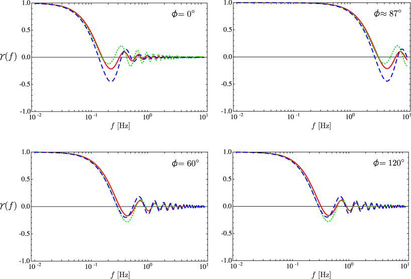
Figure 8: Overlap reduction functions of the correlation between interferometers in cluster A and B (AB link) in the case II. The orientations of the interferometers are selected as $\sigma_{A}=\sigma_{B}=0$. The tilt of the orbit is fixed to $D_{\rm{max}}/L=10^{3}$. Solid (red), dotted (green), and dashed (blue) curves correspond to the tensor, vector, and scalar modes, respectively.

The examples of the overlap reduction function for each polarization mode are shown in Fig. 8, where the parameters of the detector configuration are specifically chosen as $\sigma_{A}=\sigma_{B}=0$ and $D_{\rm{max}}/L=10^{3}$, and the results are shown for $\phi=0^{\circ}$ (top left), $60^{\circ}$ (bottom left), $87^{\circ}$ (top right), and $120^{\circ}$ (bottom right). The distance between clusters A and B becomes maximum at $\phi=0^{\circ}$ and $180^{\circ}$, and is minimum at $\phi=90^{\circ}$ and $270^{\circ}$. Compared to the four-cluster case, the amplitudes of overlap reductions functions at $f\sim 0.1$ Hz become even larger for each polarization mode. This implies that the separate detection of polarized GWBs is achievable with high SNR.

As examined in the four-cluster configuration, we consider the condition for a separate detection of three polarization modes. For small $\psi\ll 1$, Eqs. (LABEL:eq31)-(84) become

$$\left(\begin{array}[]{c}\Theta_{1,2}^{T}\\ \Theta_{1,2}^{V}\\ \Theta_{1,2}^{S}\end{array}\right) = -\frac{45}{16}\left(\begin{array}[]{c}j_{4}\\ -4j_{4}\\ 6j_{4}\end{array}\right)\cos 4\phi\;,$$ (91)

$$\left(\begin{array}[]{c}\Theta_{3}^{T}\\ \Theta_{3}^{V}\\ \Theta_{3}^{S}\end{array}\right) = 16\left(\begin{array}[]{c}j_{0}+\frac{5}{28}j_{2}-\frac{37}{1792}j_{4}\vspace{.5em}\\ j_{0}-\frac{5}{56}j_{2}+\frac{37}{448}j_{4}\vspace{.5em}\\ j_{0}-\frac{5}{28}j_{2}-\frac{111}{896}j_{4}\end{array}\right)\;,$$ (98)

$$\left(\begin{array}[]{c}\Theta_{4}^{T}\\ \Theta_{4}^{V}\\ \Theta_{4}^{S}\end{array}\right) = 16\sqrt{3}\,\psi\sin\phi$$ (106)

$$\times\left(\begin{array}[]{c}j_{0}+\frac{25}{56}j_{2}-\frac{3}{448}j_{4}\vspace{.5em}\\ j_{0}-\frac{25}{112}j_{2}+\frac{3}{112}j_{4}\vspace{.5em}\\ j_{0}-\frac{25}{56}j_{2}-\frac{9}{224}j_{4}\end{array}\right)\;.$$

Thus, for $\alpha\ll 1$, the terms $j_{2}$ and $j_{4}$ become negligible, and the overlap reduction functions for all polarization modes are reduced to an identical form. Hence, $j_{0}\sim j_{2}\sim j_{4}$ is required for having the different oscillatory behaviors for overlap reduction function of scalar, vector, and tensor modes and leads to the same conclusion as that in case I configuration, $D>\lambda_{g}$ for each pair of detectors.

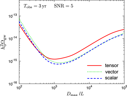
Figure 9: Detectable $h_{0}^{2}\Omega_{\rm{gw}}$ ($\xi h_{0}^{2}\Omega_{\rm{gw}}$ for the scalar mode) after the mode separation in the case II.

III.2.3 Results

For two-cluster configuration, we have, in total, 9 correlation signals between clusters A and B. Combining these signals, the optimal SNR is computed taking account of the time variation of the overlap reduction functions. In practice, the time integral in Eq. (18) is discretized as the sum of the finite time segment. We checked that the results remain unchanged if the number of segments in one year is larger than twelve.

In Fig. 9, minimum detectable amplitude $h_{0}^{2}\Omega_{\rm{gw}}$ is plotted against the maximum separation, $D_{\rm{max}}/L$, keeping $T_{\rm{obs}}=3\,{\rm{yr}}$, and ${\rm{SNR}}=5$. The detectable amplitude for each polarization mode first decreases and begins increasing as the separation $D_{\rm{max}}$ increases. The best sensitivity is achieved at $D_{\rm{max}}/L\sim 1.4\times 10^{3}$, and the detectable amplitude for each polarization mode becomes

$$h_{0}^{2}\Omega_{\rm{gw}}^{T}=1.3\times 10^{-15},$$

$$h_{0}^{2}\Omega_{\rm{gw}}^{V}=8.5\times 10^{-16},$$

$$\xi h_{0}^{2}\Omega_{\rm{gw}}^{S}=7.4\times 10^{-16}.$$

Therefore, compared to the four-cluster configuration, the sensitivity to the separate detection of each polarization mode is greatly improved. Note, however, that the optimal sensitivity to GWBs themselves is rather degraded, compared with those when we do not consider the mode separation. This is because no colocated and coaligned cluster configuration are available in the present setup.

IV Discussion

The previous section reveals that a separate detection of three polarization modes with high signal sensitivity needs a sophisticated setup for detector configuration, but we may achieve $\Omega_{\rm gw}\sim 10^{-15}$. In this section, we briefly discuss how the results are changed for a different setup or situation.

First consider the influence of astrophysical foregrounds, which was not taken into account when we estimated the SNR. It is expected that the low-frequency side of the DECIGO could be dominated by the unresolved GWs from the white-dwarf binaries. According to the estimation by Ref. Farmer and Phinney (2003), cosmological population of white-dwarf binaries produces a large GW signal at $f\lesssim 0.2$Hz, and may act as a confusion noise. Thus, below the frequency $f_{\rm cut}=0.2$Hz, a definite detection of cosmological GWBs might not be possible.

Here, in order to examine the significance of this effect, we introduce the low-frequency cutoff in the frequency integral of Eq. (13), and estimate the SNR again. Based on this, the detectable amplitude of GWB is calculated for four- and two-cluster configurations. In Figs. 10 and 11, the dependence of the detectable energy density $h_{0}^{2}\Omega_{\rm{gw}}$ on the cutoff frequency are shown for four-cluster case with $\beta=60^{\circ}$ and $90^{\circ}$, and two-cluster setup with $D_{\rm{max}}/L=10^{3}$ and $10^{4}$, respectively. In both cases, the effect of low-frequency cutoff becomes significant as $f_{\rm cut}$ increases, but the results are not drastically changed at $f_{\rm cut}\lesssim 0.2$Hz. This is rather consistent with the results by Ref. Kudoh et al. (2006). Thus, even in the presence of confusion noise, the detectable $h_{0}^{2}\Omega_{\rm{gw}}$ remains unchanged as long as the cutoff frequency is below $0.2\,{\rm{Hz}}$. This conclusion may be rather natural because DECIGO has been designed to evade the low-frequency confusion noises.

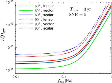
Figure 10: Detectable $h_{0}^{2}\Omega_{\rm{gw}}$ ($\xi h_{0}^{2}\Omega_{\rm{gw}}$ for the scalar mode) after the mode separation in the case I with the cutoff frequency. The detector separation is selected as $\beta=60^{\circ}$ (solid curves) and $\beta=90^{\circ}$ (dotted curves).

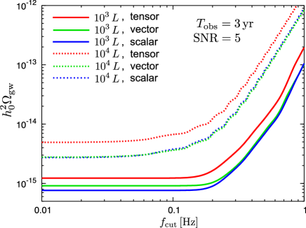
Figure 11: Detectable $h_{0}^{2}\Omega_{\rm{gw}}$ ($\xi h_{0}^{2}\Omega_{\rm{gw}}$ for the scalar mode) after the mode separation in the case II with the cutoff frequency. The detector separation is selected as $D_{\rm{max}}=10^{3}L$ (solid curves) and $10^{4}L$ (dotted curves).

Next consider the alternative design of space interferometer, i.e., BBO. As we mentioned in Sec. I, BBO plans to use a transponder type with the arm length, $L=5\times 10^{4}\,\rm{km}$. This point is rather different from DECIGO, however, the noise curve and the detector configuration of BBO are almost the same as those of DECIGO. Thus, we naively expect that the results obtained in the previous section basically hold for the case of BBO. A subtle point is that low-frequency approximation of the detector response which we adopted throughout the analysis might not be valid for GWs at frequencies $f\gtrsim 1$Hz. Thus, a correct treatment without using low-frequency approximation is necessary for quantitative estimation of detectability. Nevertheless, quantitative difference would be certainly small, and the qualitative point of our results can be applied to the BBO case, because the noise curve of BBO coincides with that of DECIGO within $5\,\%$ of a factor at frequencies below $1\,{\rm{Hz}}$ Cutler and Holz (2009) and the SNR is almost determined by a signal below $1\,{\rm{Hz}}$.

V Summary

In this paper, we discuss how well we can separately detect and measure the extra-polarization modes of a GWB in addition to the standard tensor-type GWB, i.e., scalar and vector GWBs, via the space-based interferometers. In addition to the tensor mode, scalar and vector-type GWBs may have been produced in the early stage of the Universe through various mechanisms including inflation, phase transition and reheating of the Universe, when the general relativity would not strictly hold. Thus, the detection and measurement of scalar and vector modes of GWBs is a direct probe of gravity, and can also yield information about the physics of the early universe.

We have presented the formula for optimal SNR to separately detect three polarization modes combining multiple correlation signals. Based on this, we have considered the two specific configurations for planned space interferometer, DECIGO, and estimated the ability to detect extra-polarization modes of GWB. For the four-cluster setup consisting of the four sets of spacecraft constellations with coplanar orbits, the detectable minimum amplitudes of GWB are degraded significantly for each polarization mode, and the detectable density somehow reaches $h_{0}^{2}\Omega_{\rm{gw}}\sim 10^{-14}$. This is in marked contrast to the standard analysis that only considers the tensor mode of GWB. To raise the sensitivity, we then considered the two-cluster setup, in which the orbits of two set of spacecraft constellation are slightly misaligned. Thanks to the non-stationarity of detector configuration, the cross-correlation measured at different times can be regarded as an independent set of signals with different location and separation, and this helps to improve the detection sensitivity. As a result, the detectable density is found to be $h_{0}^{2}\Omega_{\rm{gw}}\sim 10^{-15}$ for tensor mode, and even better for scalar and vector modes.

Currently, no definite theoretical bound on the amplitude of GWB exists below $h_{0}^{2}\Omega_{\rm{gw}}\sim 10^{-6}$, and thus it is rather difficult to predict how much amount of GWB is expected for each polarization mode. Nevertheless, constraints from cosmic microwave background anisotropies imply that the tensor-type GWB generated during inflation is likely to be as small as $h_{0}^{2}\Omega_{\rm{gw}}\sim 10^{-16}$ at frequency $f\sim 0.1$-$1\,{\rm{Hz}}$ Friedman et al. (2006); Chongchitnan and Efstathiou (2006); Smith et al. (2006); bib (e). Given that the coupling parameters of scalar and vector degrees of freedom to a background gravitational field are almost the same as that of the tensor, no significant amount of GWB is expected for scalar and vector polarizations. Therefore, with the setup examined in this paper, it might be hard to separately measure the three polarization modes of inflationary GWB, although the detector itself has an ability to detect such a small GWB.

Nonetheless, this argument is based on an extrapolation from the extremely low-frequency observation by 16 orders of magnitude, and there may still exist many windows to generate a large amplitude of inflationary GWB around frequency $f\sim 0.1$-$1\,{\rm{Hz}}$. Further, there are several viable scenarios that can produce a large amplitude of low-frequency GWB. An example is the GWB produced by density fluctuation through cosmological phase transition and/or preheating. In this case, the energy density of scalar GWB might exceed that of the tensor mode, because scalar GW would be easily emitted by the monopole moment of the density fluctuation. The resultant spectrum of GWB may has a sharp peak with the amplitude of at most $h_{0}^{2}\Omega_{\rm{gw}}\sim 10^{-7}$ Grojean and Servant (2007); Easther and Lim (2006); Dufaux et al. (2007); J. Garcia-Bellido and Sastre (2008); Saito and Yokoyama (2009). Hence, even with a limited sensitivity, a search for additional polarization modes of GWB via space-based interferometer is indispensable for a cosmological test of gravity, and definitely yields an additional scientific benefit for probing the physics of the early universe.

Appendix A Correlation signal in a cluster

In this Appendix, we show that it is impossible to obtain a correlation signal sensitive to a GWB in a cluster, even if three interferometers in a cluster are used.

Let us consider a correlation signal in a cluster of DECIGO like Fig. 1. We denote three spacecrafts as SC1, SC2, and SC3, three interferometers in the cluster as IFO1, IFO2, and IFO3. The displacement noise of the optical link between i-th SC and j-th SC (the light is injected from i-th SC, reflected at the mirror near j-th SC, and finally returns to i-th SC.) is $d_{ij}$ and the shot noise at i-th SC is $\zeta_{i}$. The noise components in the signal obtained by each IFO are written as

$$s_{1} = d_{12}-d_{13}+\zeta_{1}\;,$$ (107)

$$s_{2} = d_{23}-d_{21}+\zeta_{2}\;,$$ (108)

$$s_{3} = d_{31}-d_{32}+\zeta_{3}\;.$$ (109)

The displacement noises, $d_{ij}$, can be considered to be symmetric with respect to the subscripts, because the cavity storage time of light, $10L/c\approx 0.03\,{\rm{sec}}$, is shorter than the period of a GW that we are interested in, $\sim 1-10\,{\rm{sec}}$. So, Eqs. (107) - (109) can be written as

$$s_{1} = d_{12}-d_{13}+\zeta_{1}\;,$$ (110)

$$s_{2} = d_{23}-d_{12}+\zeta_{2}\;,$$ (111)

$$s_{3} = d_{13}-d_{23}+\zeta_{3}\;.$$ (112)

We linearly combine Eqs. (110) - (112) with arbitrary coefficients, and take the ensemble average of the correlation signal

$$\langle(s_{1}+c_{2}s_{2}+c_{3}s_{3})(s_{1}+c_{2}^{\prime}s_{2}+c_{3}^{\prime}s_{3})\rangle$$

$$=(1-c_{2})(1-c_{2}^{\prime})\langle d_{12}^{2}\rangle+(1-c_{3})(1-c_{3}^{\prime})\langle d_{13}^{2}\rangle$$

$$+(c_{2}-c_{3})(c_{2}^{\prime}-c_{3}^{\prime})\langle d_{23}^{2}\rangle+(1+c_{2}c_{2}^{\prime}+c_{3}c_{3}^{\prime})\langle\zeta^{2}\rangle\;.$$

Here we assumed that $\langle d_{ij}\zeta_{k}\rangle=0$, $\langle d_{ij}d_{k\ell}\rangle=0$ for $i\neq j$ and $k\neq\ell$, and $\langle\zeta_{i}\zeta_{j}\rangle=0$ for $i\neq j$, and wrote $\langle\zeta^{2}\rangle=\langle\zeta_{i}\zeta_{j}\rangle$ for $i=j$. To obtain the correlation signal that is insensitive to the correlation noise, the coefficients should be chosen as

$$(c_{2},c_{3},c_{2}^{\prime},c_{3}^{\prime})=(c_{2},-1-c_{2},1,1)\;,$$

where $c_{2}$ is arbitrary. Thus one of the combination signals in the correlation must be a symmetric combination, $s_{1}+s_{2}+s_{3}$, regardless of another combination signal.

Next, we define

$$s_{\rm{sym}}\equiv\frac{1}{\sqrt{3}}(s_{1}+s_{2}+s_{3})\;,$$

which is known as the symmetrized Sagnac signal Armstrong et al. (1999); Cornish (2001b); Prince et al. (2002), and calculate its GW signal. As we will see below, the correlation signal with $s_{\rm{sym}}$ is not helpful for the separation of the multiple polarization modes. Using Eq. (2), we can find the GW signal of $s_{\rm{sym}}$

$$h_{\rm{sym}} \equiv \frac{1}{\sqrt{3}}(h_{1}+h_{2}+h_{3})$$

$$= \sum_{p}\int_{S^{2}}d\hat{\mathbf{\Omega}}\int_{-\infty}^{\infty}df\,$$

$$\times\tilde{h}_{p}(f,\hat{\mathbf{\Omega}})\,e^{2\pi ift}\,\mathbf{D}_{\rm{sym}}:\mathbf{e}_{p}(\hat{\mathbf{\Omega}})\>,$$

where $\mathbf{D}_{\rm{sym}}$ at the zeroth order in the low frequency approximation is exactly zero since all terms are canceled due to the symmetry of the combination. To obtain the leading contribution, one needs to include the response functions in the detector arms in Eq. (4) Schilling (1997); Armstrong et al. (1999); Cornish (2001b); Rakhmanov (2008); Nishizawa et al. (2008). The detector tensor of the combination signal $s_{\rm{sym}}$ is $\mathbf{D}_{\rm{sym}}(f,\hat{\mathbf{\Omega}})\propto ifL/c$, then the GW response is suppressed below the frequency, $f\approx c/L\approx 300\,{\rm{Hz}}$. Consequently, at $0.1-1\,{\rm{Hz}}$, the GW response is $300-3000$ times worse than that before taking the signal combination.

Appendix B Derivation of optimal SNR formula for separately detecting scalar, vector and tensor polarizations

Here, we will derive the SNR formula for separately detecting the three polarization modes by optimally combining arbitrary number of detector signals ($N_{\rm{pair}}\geq 3$).

When one correlates detector signals in a frequency bin, the estimated value of the correlation signal, $\hat{\mu}_{i}(f)$, fluctuates around the true value, $\mu_{i}(f)$. Assuming the width of a frequency bin is much larger than the frequency resolution of the data we obtain, the likelihood function for $\hat{\mu}_{i}(f)$ is expected to be Gaussian distribution, owing to the central limit theorem. Let us denote a set of the estimated correlation signals of a detector pair in a frequency bin, $\{\hat{\mu}_{i}(f);1\leq i\leq N_{\rm{pair}}\}$, where the subscript $i$ designates a detector pair (for I-th and J-th detector pair, $i=IJ$). The multidimensional likelihood function for the set of the estimator is written as

$$L\bigl{[}\{\hat{\mu}_{i}(f)\}\bigr{]}\propto\exp\left[-\sum_{i=1}^{N_{\rm{pair}}}\frac{\{\hat{\mu}_{i}(f)-\mu_{i}(f)\}^{2}}{{2\cal{N}}_{i}(f)}\right]\;,$$ (114)

where the covariance noise matrix, ${\cal{N}}_{i}(f)$, is defined as, say, ${\cal{N}}_{12}(f)\equiv P_{1}(f)P_{2}(f)$. Note that we assume that detector noise is not correlated with other detectors and that a GW signal is much smaller than the noise, so the calculation in Eq. 12 is applied here.

On the other hand, from Eq. (8), the GW contribution in the correlation signal is

$$\mu_{i}(f) \propto \gamma_{i}^{T}(f)\Omega_{\rm{gw}}^{T}(f)+\gamma_{i}^{V}(f)\Omega_{\rm{gw}}^{V}(f)+\gamma_{i}^{S}(f)\xi\Omega_{\rm{gw}}^{S}(f)\;,$$

$$\hat{\mu}_{i}(f) \propto \gamma_{i}^{T}(f)\hat{\Omega}_{\rm{gw}}^{T}(f)+\gamma_{i}^{V}(f)\hat{\Omega}_{\rm{gw}}^{V}(f)+\gamma_{i}^{S}(f)\xi\hat{\Omega}_{\rm{gw}}^{S}(f)\;.$$

The hat fixed to $\Omega_{\rm{gw}}$ represents that it is the estimated quantity. Substituting Eqs. (LABEL:eq40) and (LABEL:eq41) for Eq. (114), we obtain the quadratic with respect to $\Omega_{\rm{gw}}$ in the argument of Eq. (114), from which we can read the proportional relation of the Fisher matrix

$$\mathbf{F}(f)={\rm{a\;factor}}\times\left(\begin{array}[]{ccc}F_{TT}&F_{TV}&F_{TS}\\ F_{TV}&F_{VV}&F_{VS}\\ F_{TS}&F_{VS}&F_{SS}\end{array}\right)\;,$$

with

$$F_{TT}(f) = \sum_{i}\frac{(\gamma_{i}^{T})^{2}}{{\cal{N}}_{i}}\;,\quad F_{VV}(f)=\sum_{i}\frac{(\gamma_{i}^{V})^{2}}{{\cal{N}}_{i}}\;,\quad$$ (117)

$$F_{SS}(f) = \sum_{i}\frac{(\gamma_{i}^{S})^{2}}{{\cal{N}}_{i}}\;,\quad F_{TV}(f)=\sum_{i}\frac{\gamma_{i}^{T}\gamma_{i}^{V}}{{\cal{N}}_{i}}\;,\quad$$ (118)

$$F_{VS}(f) = \sum_{i}\frac{\gamma_{i}^{V}\gamma_{i}^{S}}{{\cal{N}}_{i}}\;,\quad F_{TS}(f)=\sum_{i}\frac{\gamma_{i}^{T}\gamma_{i}^{S}}{{\cal{N}}_{i}}\;,\quad$$ (119)

Thus, we find that the SNR in a frequency bin is proportional to some combination of the components of the Fisher matrix, namely

$$\bigl{[}{\rm{SNR}}^{T}(f)\bigr{]}^{2} \propto \frac{(\Omega_{\rm{gw}}^{T})^{2}}{(\mathbf{F}^{-1})_{11}}=\frac{(\Omega_{\rm{gw}}^{T})^{2}\det\mathbf{F}}{F_{VV}F_{SS}-F_{VS}^{2}}\;,$$ (120)

$$\bigl{[}{\rm{SNR}}^{V}(f)\bigr{]}^{2} \propto \frac{(\Omega_{\rm{gw}}^{V})^{2}}{(\mathbf{F}^{-1})_{22}}=\frac{(\Omega_{\rm{gw}}^{V})^{2}\det\mathbf{F}}{F_{TT}F_{SS}-F_{TS}^{2}}\;,$$ (121)

$$\bigl{[}{\rm{SNR}}^{S}(f)\bigr{]}^{2} \propto \frac{(\xi\Omega_{\rm{gw}}^{S})^{2}}{(\mathbf{F}^{-1})_{33}}=\frac{(\Omega_{\rm{gw}}^{S})^{2}\det\mathbf{F}}{F_{TT}F_{VV}-F_{TV}^{2}}\;.$$ (122)

To determine the frequency-dependent factor of the proportional relation, we compare those with the SNR formula for $N_{\rm{pair}}=3$ case with three detectors, which has been derived in Nishizawa et al. (2009). For $N_{\rm{pair}}=3$, Eqs. (120) - (122) are reduced to

$$({\rm{SNR}}^{M}(f))^{2} \propto \left[\frac{H_{g}^{2}(f)}{H_{n}^{2}(f)}\right]^{M}\;,\quad M=T,V,S\;,$$

$$\mathbf{\Pi}(f)\equiv\left(\begin{array}[]{ccc}\gamma^{T}_{12}&\gamma^{V}_{12}&\gamma^{S}_{12}\\ \gamma^{T}_{23}&\gamma^{V}_{23}&\gamma^{S}_{23}\\ \gamma^{T}_{31}&\gamma^{V}_{31}&\gamma^{S}_{31}\end{array}\right)\;,$$

$$\left[\frac{H_{g}^{2}(f)}{H_{n}^{2}(f)}\right]^{T} = \frac{(\Omega_{\rm{gw}}^{T})^{2}(\det\mathbf{\Pi})^{2}}{P_{1}P_{2}(\gamma_{23}^{V}\gamma_{31}^{S}-\gamma_{23}^{S}\gamma_{31}^{V})^{2}+P_{2}P_{3}(\gamma_{31}^{V}\gamma_{12}^{S}-\gamma_{31}^{S}\gamma_{12}^{V})^{2}+P_{3}P_{1}(\gamma_{12}^{V}\gamma_{23}^{S}-\gamma_{12}^{S}\gamma_{23}^{V})^{2}}\;,$$

$$\left[\frac{H_{g}^{2}(f)}{H_{n}^{2}(f)}\right]^{V} = \frac{(\Omega_{\rm{gw}}^{V})^{2}(\det\mathbf{\Pi})^{2}}{P_{1}P_{2}(\gamma_{23}^{S}\gamma_{31}^{T}-\gamma_{23}^{T}\gamma_{31}^{S})^{2}+P_{2}P_{3}(\gamma_{31}^{S}\gamma_{12}^{T}-\gamma_{31}^{T}\gamma_{12}^{S})^{2}+P_{3}P_{1}(\gamma_{12}^{S}\gamma_{23}^{T}-\gamma_{12}^{T}\gamma_{23}^{S})^{2}}\;,$$

$$\left[\frac{H_{g}^{2}(f)}{H_{n}^{2}(f)}\right]^{S} = \frac{(\xi\Omega_{\rm{gw}}^{S})^{2}(\det\mathbf{\Pi})^{2}}{P_{1}P_{2}(\gamma_{23}^{T}\gamma_{31}^{V}-\gamma_{23}^{V}\gamma_{31}^{T})^{2}+P_{2}P_{3}(\gamma_{31}^{T}\gamma_{12}^{V}-\gamma_{31}^{V}\gamma_{12}^{T})^{2}+P_{3}P_{1}(\gamma_{12}^{T}\gamma_{23}^{V}-\gamma_{12}^{V}\gamma_{23}^{T})^{2}}\;.$$

On the other hand, according to Nishizawa et al. (2009), the SNR formula in $N_{\rm{pair}}=3$ case (A factor coming from non-orthogonal arms, $\sin\chi^{2}=3/4$, is corrected.) is given by

$${\rm{SNR}}=\frac{9H_{0}^{2}}{40\pi^{2}}\sqrt{T_{\rm{obs}}}\biggl{[}2\int_{0}^{\infty}df\frac{H_{g}^{2}(f)}{f^{6}H_{n}^{2}(f)}\biggr{]}^{1/2}\;.$$ (124)

Comparing Eq. (LABEL:eq44) with Eq. (124) and compensating the proportional factor, and then integrating with respect to frequency, we finally obtain

$${\rm{SNR}}^{M} = \frac{9H_{0}^{2}}{40\pi^{2}}\sqrt{T_{\rm{obs}}}\biggl{[}2\int_{0}^{\infty}df\frac{(\Omega_{\rm{gw}}^{M}(f))^{2}\det\mathbf{F}(f)}{f^{6}{\cal{F}}_{M}(f)}\biggr{]}^{1/2}\;,$$

where we redefined the Fisher matrix, $\mathbf{F}$, as the matrix

$$\mathbf{F}(f)\equiv\left(\begin{array}[]{ccc}F_{TT}&F_{TV}&F_{TS}\\ F_{TV}&F_{VV}&F_{VS}\\ F_{TS}&F_{VS}&F_{SS}\end{array}\right)\;.$$

The quantity ${\cal{F}}_{M}$ is the determinant of the sub-matrix, which is constructed by removing the $M$’s elements from (new) $\mathbf{F}$.

Although so far we implicitly assume that the overlap reduction functions are time-independent, the overlap reduction functions actually depend on time in the case of a space-based detector though its orbital motion. It is easy to extend to time-dependent overlap reduction function. In Eq. (LABEL:eq72), the overlap reduction functions are included through Eqs. (117) - (119). As long as a stochastic GWB is stationary, the summation with respect to $i$ is equivalent to the integral with respect to time, because the correlation signals at different times can be regarded as those of the detector pairs which have different location and orientation. Therefore, Eq. (LABEL:eq72) and Eqs. (117) - (119) should be replaced with

$${\rm{SNR}}^{M} = \frac{9H_{0}^{2}}{40\pi^{2}}\biggl{[}2\int_{0}^{\infty}df\frac{(\Omega_{\rm{gw}}^{M}(f))^{2}\det\mathbf{F}(f)}{f^{6}{\cal{F}}_{M}(f)}\biggr{]}^{1/2}$$

and

$$F_{MM^{\prime}}(f)=\sum_{i}\int_{0}^{T_{\rm{obs}}}dt\,\frac{\gamma_{i}^{M}(t,f)\gamma_{i}^{M^{\prime}}(t,f)}{{\cal{N}}_{i}(f)}\;,$$

where $M$ and $M^{\prime}$ denote polarization modes, $M,M^{\prime}=T,V,S$.

References

- Grishchuk (1974) L. P. Grishchuk, Sov. Phys. JETP 40, 409 (1974).
- Rubakov et al. (1982) V. A. Rubakov, M. V. Sazhin, and A. V. Veryaskin, Phys. Lett. B 115, 189 (1982).
- Abbott and Wise (1984) L. F. Abbott and M. B. Wise, Nucl. Phys. B 244, 541 (1984).
- Allen (1988) B. Allen, Phys. Rev. D 37, 2078 (1988).
- Kosowsky et al. (1992) A. Kosowsky, M. S. Turner, and R. Watkins, Phys. Rev. D 45, 4514 (1992).
- Kamionkowski et al. (1994) M. Kamionkowski, A. Kosowsky, and M. S. Turner, Phys. Rev. D 49, 2837 (1994).
- Grojean and Servant (2007) C. Grojean and G. Servant, Phys. Rev. D 75, 043507 (2007).
- Kahniashvili et al. (2008) T. Kahniashvili, A. Kosowsky, G. Gogoberidze, and Y. Maravin, Phys. Rev. D 78, 043003 (2008).
- Khlebnikov and Tkachev (1997) S. Khlebnikov and I. Tkachev, Phys. Rev. D 56, 653 (1997).
- Easther and Lim (2006) R. Easther and E. A. Lim, J. Cosmol. Astropart. Phys. 04, 010 (2006).
- Dufaux et al. (2007) J. F. Dufaux, A. Bergman, G. Felder, L. Kofman, and J. P. Uzan, Phys. Rev. D 76, 123517 (2007).
- Garcia-Bellido and Figueroa (2007) J. Garcia-Bellido and D. G. Figueroa, Phys. Rev. Lett. 98, 061302 (2007).
- J. Garcia-Bellido and Sastre (2008) D. G. F. J. Garcia-Bellido and A. Sastre, Phys. Rev. D 77, 043517 (2008).
- bib (a) C. M. Will, Theory and experiment in gravitational physics, (Cambridge University Press (1993).
- Eardley et al. (1973) D. M. Eardley, D. L. Lee, A. P. Lightman, R. V. Wagoner, and C. M. Will, Phys. Rev. Lett. 30, 884 (1973).
- Brans and Dicke (1961) C. Brans and R. H. Dicke, Phys. Rev. 124, 925 (1961).
- bib (b) Y. Fujii and K. Maeda, The Scalar-Tensor Theory of Gravitation, (Cambridge University Press (2002).
- bib (c) T. P. Sotiriou and V. Faraoni, arXiv:0805.1726.
- Capozziello et al. (2009) S. Capozziello, M. D. Laurentis, S. Nojiri, and S. D. Odintsov, Gen. Relativ. Gravit. 41, 2313 (2009).
- Alves et al. (2009) M. E. S. Alves, O. D. Miranda, and J. C. N. de Araujo, Phys. Lett. B 679, 401 (2009).
- bib (d) M. E. S. Alves, O. D. Miranda, and J. C. N. de Araujo, arXiv:1004.5580 (2010).
- Dvali et al. (2000) G. Dvali, G. Gabadadze, and M. Porrati, Phys. Lett. B 485, 208 (2000).
- bib (e) E. Komatsu and others, arXiv:1001.4538 (2010).
- bib (f) The LIGO Scientific Collaboration and The Virgo Collaboration, Nature 460, 990 (2009).
- Lee et al. (2008) K. J. Lee, F. A. Jenet, and R. H. Price, Astrophys. J. 685, 1304 (2008).
- Seto et al. (2001) N. Seto, S. Kawamura, and T. Nakamura, Phys. Rev. Lett. 87, 221103 (2001).
- bib (g) S. Sato et al., Journal of Physics: Conference Series 154, 012040 (2009).
- bib (h) E. S. Phinney et al., Big Bang Observer Mission Concept Study (NASA, 2003).
- Cutler and Holz (2009) C. Cutler and D. E. Holz, Phys. Rev. D 80, 104009 (2009).
- bib (i) In general gravity theory, massive gravitons propagate with the speed less than . However, the observation of the binary pulsars has tightly constrained the propagating speed of gravitons to be bib (l). So, we set , which hardly affects the cross-correlation analysis.
- Allen and Ottewill (1997) B. Allen and A. C. Ottewill, Phys. Rev. D 56, 545 (1997).
- Cornish (2001a) N. J. Cornish, Class. Quantum Grav. 18, 4277 (2001a).
- Kudoh and Taruya (2005) H. Kudoh and A. Taruya, Phys. Rev. D 71, 024025 (2005).
- Taruya and Kudoh (2005) A. Taruya and H. Kudoh, Phys. Rev. D 72, 104015 (2005).
- Kudoh et al. (2006) H. Kudoh, A. Taruya, T. Hiramatsu, and Y. Himemoto, Phys. Rev. D 73, 064006 (2006).
- Taruya (2006) A. Taruya, Phys. Rev. D 74, 104022 (2006).
- Thrane et al. (2009) E. Thrane, S. Ballmer, J. D. Romano, S. Mitra, D. Talukder, S. Bose, and V. Mandic, Phys. Rev. D 80, 122002 (2009).
- Drasco and Flanagan (2003) S. Drasco and E. E. Flanagan, Phys. Rev. D 67, 082003 (2003).
- Himemoto et al. (2007) Y. Himemoto, A. Taruya, H. Kudoh, and T. Hiramatsu, Phys. Rev. D 75, 022003 (2007).
- Seto (2008) N. Seto, Astrophys. J. 683, L95 (2008).
- Maggiore (2000) M. Maggiore, Phys. Rep. 331, 283 (2000).
- Allen and Romano (1999) B. Allen and J. D. Romano, Phys. Rev. D 59, 102001 (1999).
- bib (j) If a theory contains a parity-violating term, and modes are polarized. Such a model predicts a GWB with circular polarizations. The detectability has been discussed in Seto and Taruya (2008); Seto (2007, 2006); Seto and Taruya (2007).
- Christensen (1992) N. Christensen, Phys. Rev. D 46, 5250 (1992).
- Flanagan (1993) E. E. Flanagan, Phys. Rev. D 48, 2389 (1993).
- Nishizawa et al. (2009) A. Nishizawa, A. Taruya, K. Hayama, S. Kawamura, and M. Sakagami, Phys. Rev. D 79, 082002 (2009).
- bib (k) That is calculated with DECIGO design parameters, assuming the noise curve is quantum-noise limited. The parameters we used are the arm length , the angular frequency of a laser , the laser power , the mirror mass , and the finesse of the cavity 10.
- Seto and Taruya (2008) N. Seto and A. Taruya, Phys. Rev. D 77, 103001 (2008).
- Holz and Hughes (2005) D. E. Holz and S. A. Hughes, Astrophys. J. 629, 15 (2005).
- Seto (2007) N. Seto, Phys. Rev. D 75, 061302(R) (2007).
- Farmer and Phinney (2003) A. J. Farmer and E. S. Phinney, Mon. Not. R. Astron. Soc. 346, 1197 (2003).
- Friedman et al. (2006) B. C. Friedman, A. Cooray, and A. Melchiorri, Phys. Rev. D 74, 123509 (2006).
- Chongchitnan and Efstathiou (2006) S. Chongchitnan and G. Efstathiou, Phys. Rev. D 73, 083511 (2006).
- Smith et al. (2006) T. L. Smith, H. V. Peiris, and A. Cooray, Phys. Rev. D 73, 123503 (2006).
- Saito and Yokoyama (2009) R. Saito and J. Yokoyama, Phys. Rev. Lett. 102, 161101 (2009).
- Armstrong et al. (1999) J. W. Armstrong, F. B. Estabrook, and M. Tinto, Astrophys. J. 527, 814 (1999).
- Cornish (2001b) N. J. Cornish, Phys. Rev. D 65, 022004 (2001b).
- Prince et al. (2002) T. A. Prince, M. Tinto, S. L. Larson, and J. W. Armstrong, Phys. Rev. D 66, 122002 (2002).
- Schilling (1997) R. Schilling, Class. Quantum Grav. 14, 1513 (1997).
- Rakhmanov (2008) M. Rakhmanov, Class. Quantum Grav. 25, 184017 (2008).
- Nishizawa et al. (2008) A. Nishizawa et al., Phys. Rev. D 77, 022002 (2008).
- bib (l) L. S. Finn and P. J. Sutton, Phys. Rev. D 65, 044022 (2002).
- Seto (2006) N. Seto, Phys. Rev. Lett. 97, 151101 (2006).
- Seto and Taruya (2007) N. Seto and A. Taruya, Phys. Rev. Lett. 99, 121101 (2007).
- Will (2006) C. M. Will, Living Rev. Relativity 9, 3 (2006).