Secular momentum transport by gravitational waves from spinning compact binaries

Zoltán Keresztes1,2⋆    Balázs Mikóczi3†    László Á. Gergely1,2,4‡    Mátyás Vasúth 1 Department of Theoretical Physics, University of Szeged, Tisza Lajos krt 84-86, Szeged 6720, Hungary
2 Department of Experimental Physics, University of Szeged, Dóm tér 9, Szeged 6720, Hungary
3 KFKI Research Institute for Particle and Nuclear Physics, Budapest 114, P.O.Box 49, H-1525 Hungary
4 Institute for Advanced Study, Collegium Budapest, Szentháromság u 2, Budapest 1014, Hungary
zkeresztes@titan.physx.u-szeged.hu mikoczi@rmki.kfki.hu  gergely@physx.u-szeged.hu vasuth@rmki.kfki.hu
Abstract

We present a closed system of coupled first order differential equations governing the secular linear momentum loss of a compact binary due to emitted gravitational waves, with the leading order relativistic and spin-orbit perturbations included. In order to close the system, the secular evolution equations of the linear momentum derived from the dissipative dynamics are supplemented with the secular evolutions of the coupled angular variables, as derived from the conservative dynamics.

1 Introduction

The inspiral of compact objects in binary systems is driven by the emitted gravitational radiation which carries energy, angular and linear momenta away from the source. Global conservation of these quantities implies a radiative orbital evolution, including a possible recoil of the system. The energy and magnitude of orbital angular momentum of the binary determine the quasi-Keplerian orbit in the post-Newtonian (PN) regime. These quantities are known to high accuracy for binaries on eccentric orbits, with PN, spin-orbit (SO), spin-spin (SS), mass quadrupole - mass dipole (QM) and magnetic dipole - magnetic dipole (DD) coupling terms [1]. Moreover, the orientation of the (quasi-precessing) plan of motion, defined by the direction of the Newtonian orbital angular momentum, is known to high accuracy with all the above-mentioned contributions.

Due to asymmetries in the configuration of the source the radiation is often emitted anisotropically. The linear momentum loss of the binary leads to the recoil of the center of mass in the opposite direction, which in extreme situations results the kick-off of the binary from its host galaxy. This effect, however, vanishes for equal mass binaries due to the fact that the leading order relativistic contribution to the linear momentum loss scales with the mass difference $\delta m=m_{1}-m_{2}$ of the orbiting bodies.

The gravitational recoil of a binary system and the classical linear momentum loss of the final black hole were discussed in [2, 3] with the inclusion of the lowest multipoles needed for the computation of momentum ejection. The first quasi-Keplerian analytic studies were given in [4], where the linear momentum flux of gravitational waves from a binary system of two point masses in Keplerian orbit were calculated. 1 PN corrections to the gravitational recoil were discussed in [5], while 2PN recoil effects for binaries on quasicircular orbits in [6]. Several numerical estimates for the kick velocity of non-spinning binaries were given, e.g. in [7, 8, 9], with the maximum recoil in this case found as $\sim 175$ km/s [10]. Recently it has been shown [11], that the ringdown phase acts as an anti-kick as compared to the inspiral and plunge, the global result being consistent with the numerical estimates.

The rotation of the components adds however additional structure to the emitted radiation and recoil. Spin contributions to the linear momentum loss are analyzed in [12], and more recently in [13]. The SO contributions scale with the magnitude of spins which could be high for galactic black holes. Numerical analyses indicate that significant gravitational recoil can be obtained in spinning binaries [14, 15, 16, 17, 18] even with a high degree of symmetry in the configuration, i.e. for equal-mass binaries with antialigned initial spins in the orbital plane [19]. In a detailed review [20], Racine, Buonanno and Kidder have computed the instantaneous linear momentum flux emitted by spinning binaries at 2PN order with the inclusion of the next-to-leading order SO, SO tail and SS terms. Moreover, the recoil velocity as a function of the orbital frequency was given for quasicircular orbits.

In the present work we give the previously unknown secular expressions for the linear momentum loss of an inspiralling binary system, with the inclusion of leading order relativistic and SO contributions. The analytic approach presented here is suitable for characterize analytically the dependence of the recoil on binary parameters.

Section 2 contains elements of the conservative dynamics with the inclusion of first post-Newtonian and spin-orbit contributions. At the end of the section the secular conservative evolution of the relevant angle variables is given. In Section 3 we start from the expressions of the SO contributions to the instantaneous linear momentum loss given in [12], then we derive the dissipative secular linear momentum evolution. The two sets of secular evolutions couple to a closed system of first order differential equations.

The secular evolutions are derived as follows: first we rewrite the instantaneous evolutions in terms of the radial parametrization of quasi-Keplerian orbits [1]. As a result, all the radial functional dependencies are expressed in terms of a single variable $\chi$, the generalized true anomaly. Averaging these expressions over a radial period becomes particularly straightforward in terms of the complex version of $\chi$, which renders the problem to the computation of residues in the origin of the complex parameter plane [21, 22]. This procedure smears out short timescale effects and we obtain a simpler dynamics, suitable for monitoring the secular changes. The procedure is similar to our previous computations of the SO-induced secular changes of the energy, magnitude of orbital angular momentum and relative angles among the orbital angular momentum and spins [23]. An additional difficulty in the present computation arises from the vectorial character of the linear momentum, and the subsequent system of coupled differential equations.

Our description is generic, being valid for generic (non-circular, non-spherical) orbits.

Notation. For any vector $\mathbf{V}$ its magnitude is denoted as $V$ and its direction (a unit vector) as $\mathbf{\hat{V}}$.

2 Elements of the conservative dynamics

In this section we derive useful elements of the conservative dynamics, originating from the SO coupling. We derive the result in terms of:

(a) the physical parameters of the binary: total mass $m=m_{1}+m_{2}$, mass ratio ${\nu=m}_{2}/m_{1}\leq 1$, symmetric mass ratio $\eta=\mu/m$ (where $\mu=m_{1}m_{2}/m$ is the reduced mass), dimensionless spin parameters $\chi_{i}=\left(G/c\right)^{-1}S_{i}/m_{i}^{2}$

(b) dynamical constants of motion: the energy $E$, the magnitude $L$ of the orbital angular momentum $\mathbf{L}$ and $A=\left(G^{2}m^{2}\mu^{2}+{2EL^{2}/\mu}\right)^{1/2}$ (this would be the length of the Laplace-Runge-Lenz vector of the Keplerian motion characterized by $E$ and $\mathbf{L}$)

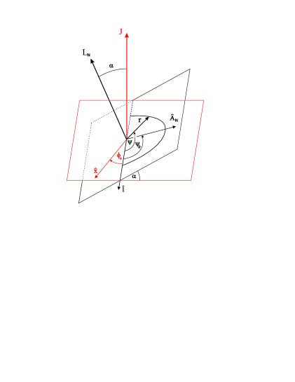
(c) angular variables related to the orbital momenta: the relative angles of spins among themselves $\gamma$ and with the orbital angular momentum $\kappa_{i}$, the polar angles $\psi_{i}$ of the spins in the plane of motion (measured from the intersection $\mathbf{\hat{l}}$ of the plane of motion with the plane perpendicular to the total angular momentum $\mathbf{J=L+S}$, where $\mathbf{S=S}_{\mathbf{1}}+\mathbf{S}_{\mathbf{2}}$), and

(d) angular variables characterizing the orbit: the inclination $\alpha$ of the orbital plane with respect to the plane perpendicular to $\mathbf{J}$, the angle $\phi_{n}$ between $\mathbf{\hat{l}}$ and an inertial axis $\mathbf{\hat{x}}$ taken in the plane perpendicular to $\mathbf{J}$, finally the angle $\psi_{p}$ span by the periastron $\mathbf{\hat{A}}_{\mathbf{N}}$ and $\mathbf{\hat{l}}$ (see Fig 1). These three angles will be referred occasionally as Euler angles, as three consecutive rotations with $\phi_{n},~{}\alpha$ and $\psi_{p}$ about the axes $z,~{}x$ and again $z$ transform from an inertial system with $\mathbf{\hat{J}}$ as the  $z\,$-axis to the system with the $x$-axis pointing towards the periastron and the $y$-axis in the plane of motion.

Refer to caption
Figure 1: The angular variables.

2.1 Lagrangian dynamics

The Lagrangian characterizing the dynamics to 1.5 PN orders (tail terms are omitted) is

$$\mathcal{L}=\mathcal{L}_{N}+\mathcal{L}_{PN}+\mathcal{L}_{SO}\ ,$$ (1)

with the contributions

$\displaystyle\mathcal{L}_{N}$ $\displaystyle=$ $\displaystyle\frac{\mu\mathbf{v}^{2}}{2}+\frac{Gm\mu}{r}\ ,$
$\displaystyle\mathcal{L}_{PN}$ $\displaystyle=$ $\displaystyle\frac{1}{8c^{2}}\left(1-3\eta\right)\mu v^{4}+\!\frac{Gm\mu}{2rc^{2}}\!\left[\!\left(3\!+\!\eta\right)v^{2}\!+\!\eta\dot{r}^{2}\!-\!\frac{Gm}{r}\!\right]\ ,$
$\displaystyle\mathcal{L}_{SO}$ $\displaystyle=$ $\displaystyle\frac{G\mu}{2c^{2}r^{3}}\mathbf{v}\cdot[\mathbf{r}\times(4\mathbf{S}+3{\mbox{\boldmath$\sigma$}})]\ .$ (2)

Here ${\mbox{\boldmath$\sigma$}=\nu}\mathbf{S}_{\mathbf{1}}+{\nu}^{-1}\mathbf{S}_{\mathbf{2}}$ is the mass-weighted spin vector. The SO part of the Lagrangian applies to the Newton-Wigner spin supplementary condition and was given first in Ref. [1]. The Lagrangian gives

$$\mathbf{a}=\mathbf{a}_{\mathbf{N}}+\mathbf{a}_{\mathbf{PN}}+\mathbf{a}_{\mathbf{SO}}\ ,$$ (3)

with

$\displaystyle\mathbf{a}_{\mathbf{N}}$ $\displaystyle=$ $\displaystyle-\frac{Gm}{r^{3}}\mathbf{r}\ ,$ (4)
$\displaystyle\mathbf{a}_{\mathbf{PN}}$ $\displaystyle=$ $\displaystyle-\frac{Gm}{c^{2}r^{3}}\left\{\mathbf{r}\left[\left(1+3\eta\right)\mathbf{v}^{2}-2\left(2+\eta\right)\frac{Gm}{r}-\frac{3}{2}\eta\dot{r}^{2}\right]-2\left(2-\eta\right)r\dot{r}\mathbf{v}\right\}\ ,$ (5)
$\displaystyle\mathbf{a}_{\mathbf{SO}}$ $\displaystyle=$ $\displaystyle\frac{G}{c^{2}r^{3}}\left[\frac{3}{2r^{2}}\mathbf{r}\left[\left(\mathbf{r}\times\mathbf{v}\right)\cdot\left(4\mathbf{S}+3{\mbox{\boldmath$\sigma$}}\right)\right]+\frac{3}{2}\frac{\dot{r}}{r}\mathbf{r}\times\left(4\mathbf{S}+3{\mbox{\boldmath$\sigma$}}\right)-\mathbf{v}\times\left(4\mathbf{S}+3{\mbox{\boldmath$\sigma$}}\right)\right]\ .$ (6)

2.2 Constants of motion

The constants of motion are the energy $E$ and the total angular momentum $\mathbf{J}$. As the total orbital angular momentum undergoes a pure precessional motion [24, 25], its magnitude $L$ is also a conserved quantity.

The total orbital angular momentum $\mathbf{L=r\times}\left(\partial\mathcal{L}/\partial\mathbf{v}\right)$ can be decomposed as

$$\mathbf{L}=\mathbf{L}_{\mathbf{N}}+\mathbf{L}_{\mathbf{PN}}+\mathbf{L}_{\mathbf{SO}}\ ,$$ (7)

with

$\displaystyle\mathbf{L_{N}}$ $\displaystyle=$ $\displaystyle\mu\mathbf{r}\times\mathbf{v}\ ,$ (8)
$\displaystyle\mathbf{L_{PN}}$ $\displaystyle=$ $\displaystyle\mathbf{L_{N}}\left[\frac{\left(1-3\eta\right)}{2}\frac{\mathbf{v}^{2}}{c^{2}}+\left(3\!+\!\eta\right)\!\frac{Gm}{c^{2}r}\right]\ ,$ (9)
$\displaystyle\mathbf{L_{SO}}$ $\displaystyle=$ $\displaystyle\frac{G\mu}{2c^{2}r^{3}}\mathbf{r}\times\left[\mathbf{r}\times\left(4\mathbf{S}+3{\mbox{\boldmath$\sigma$}}\right)\right]\ .$ (10)

We note here the useful approximate relation

$$L^{2}={L}_{N}^{2}+\lambda_{PN}+\lambda_{SO}\ ,$$ (11)

where

$\displaystyle\lambda_{PN}$ $\displaystyle\equiv$ $\displaystyle 2\mathbf{L}_{\mathbf{N}}\cdot\mathbf{L}_{\mathbf{PN}}=2{L}^{2}\left[\left(1-3\eta\right)\frac{E}{c^{2}}+2\left(2-\eta\right)\!\frac{Gm\mu}{c^{2}r}\right]\ ,$ (12)
$\displaystyle\lambda_{SO}$ $\displaystyle\equiv$ $\displaystyle 2\mathbf{L}_{\mathbf{N}}\cdot\mathbf{L}_{\mathbf{SO}}=-\frac{G\mu L}{c^{2}r}\sum\limits_{i=1,j\neq i}^{2}\!\frac{4m_{i}+3m_{j}}{m_{i}}S_{i}\cos\kappa_{i}\ .$ (13)

2.3 The evolutions of $\psi$ and $\phi_{n}$

The polar and azimuthal angles $\theta,\varphi$ of the reduced mass particle in the inertial system with $\mathbf{\hat{J}}$ as the  $z\,$-axis can be related to the Euler angles ($\phi_{n},~{}\alpha,~{}\psi$) characterizing a non-inertial reference system with the $x$-axis at the location of the reduced mass particle and the $y$-axis in the plane of motion [26]:

$\displaystyle\sin\theta\cos\varphi$ $\displaystyle=$ $\displaystyle\cos\alpha\sin\phi_{n}\sin\psi+\cos\phi_{n}\cos\psi\ ,$ (14)
$\displaystyle\sin\theta\sin\varphi$ $\displaystyle=$ $\displaystyle\cos\alpha\cos\phi_{n}\sin\psi-\sin\phi_{n}\cos\psi\ ,$ (15)
$\displaystyle\cos\theta$ $\displaystyle=$ $\displaystyle\sin\alpha\sin\psi\ .$ (16)

Tedious but straightforward algebra leads to

$\displaystyle\dot{\psi}$ $\displaystyle=$ $\displaystyle\cos\alpha\ \dot{\varphi}-\frac{\sin\alpha\cos\psi}{\sin\theta}\ \dot{\theta}+\cos\alpha\ \dot{\phi}_{n}\ ,$
$\displaystyle\dot{\phi}_{n}$ $\displaystyle=$ $\displaystyle-\dot{\varphi}-\frac{\cot\alpha}{\sin\theta\cos\psi}\ \dot{\theta}+\frac{\tan\psi}{\sin^{2}\alpha}\frac{d}{dt}\left(\cos\alpha\right)~{}\ .$ (17)

The Newtonian orbital angular momentum, expressed in terms of ($\theta$, $\varphi$) gives

$$L_{N}^{2}={\mu^{2}}r^{4}(\dot{\theta}^{2}+\sin^{2}\theta\ \dot{\varphi}^{2})\ ,\quad\left(\mathbf{L_{N}}\right)_{z}={\mu}r^{2}\sin^{2}\theta\ \dot{\varphi}\ .$$ (18)

By employing Eqs. (11), (16) and $\left(\mathbf{L_{N}}\right)_{z}=L_{N}\cos\alpha$ we obtain the evolutions:

$\displaystyle\sin\theta~{}\dot{\theta}$ $\displaystyle=$ $\displaystyle-\frac{L}{{\mu}r^{2}}\sin\alpha\cos\psi\left(1-\frac{\lambda_{PN}+\lambda_{SO}}{2{L}^{2}}\right)\ ,$ (19)
$\displaystyle\sin^{2}\theta~{}\dot{\varphi}$ $\displaystyle=$ $\displaystyle\frac{L}{{\mu}r^{2}}\cos\alpha\left(1-\frac{\lambda_{PN}+\lambda_{SO}}{2L^{2}}\right)\ .$ (20)

The minus sign in the first equation was chosen after taking the square root in such a way that when we insert these equations into Eqs. (17), we obtain

$\displaystyle\dot{\psi}$ $\displaystyle=$ $\displaystyle\frac{L}{{\mu}r^{2}}\left(1-\frac{\lambda_{PN}+\lambda_{SO}}{2{L}^{2}}\right)+\dot{\phi}_{n}\cos\alpha\ \ ,$ (21)
$\displaystyle\dot{\phi}_{n}$ $\displaystyle=$ $\displaystyle\frac{\tan\psi}{\sin^{2}\alpha}\frac{d}{dt}\left(\cos\alpha\right)\ ,$ (22)

which reduce to the correct equations $\dot{\psi}=L/\mu r^{2}$ and $\phi_{n}=$const at Newtonian order.

Provided that we can obtain $\dot{\alpha}$ by a complementary method, the evolutions of $\psi$ and $\phi_{n}$ can be given explicitly. This will be done in the following subsection.

2.4 The evolution of the orbital inclination

From $\cos\alpha=\mathbf{\hat{J}}\cdot\mathbf{\hat{L}}_{\mathbf{N}}$, as $\mathbf{J}$ is conserved, we get

$$\frac{d}{dt}\left(\cos\alpha\right)=\mathbf{\hat{J}}\cdot\frac{d}{dt}\left(\mathbf{\hat{L}}_{\mathbf{N}}\right)\ .$$ (23)

Employing Eq. (3) gives

$$\mathbf{\dot{L}}_{\mathbf{N}}=\mu\mathbf{r}\times\mathbf{a=}\ \frac{2Gm}{c^{2}r^{2}}\left(2-\eta\right)\dot{r}\mathbf{L}_{\mathbf{N}}+\frac{G\mu}{c^{2}r^{3}}\left\{\left(\frac{3}{2}\frac{\dot{r}}{r}\ \mathbf{r}-\mathbf{v}\right)\left[\mathbf{r}\cdot\left(4\mathbf{S}+3{\mbox{\boldmath$\sigma$}}\right)\right]-\frac{r\dot{r}}{2}\left(4\mathbf{S}+3{\mbox{\boldmath$\sigma$}}\right)\right\}\ .$$ (24)

From here we can derive the time derivative of $\mathbf{\hat{L}}_{\mathbf{N}}$. We then find that the leading order evolution of $\alpha$ is of order $S^{2}/JL$:

$\displaystyle\frac{d}{dt}\left(\cos\alpha\right)$ $\displaystyle=$ $\displaystyle\frac{G\mu\dot{r}}{2c^{2}JLr^{2}}\left[\left(4+3\nu\right)S_{1}\cos\kappa_{1}+\left(4+3\nu^{-1}\right)S_{2}\cos\kappa_{2}\right]\left(S_{1}\cos\kappa_{1}+S_{2}\cos\kappa_{2}\right)$ (25)
$\displaystyle-\frac{G\mu\dot{r}}{2c^{2}JLr^{2}}\left\{\left(4+3\nu\right)S_{1}^{2}+\left[8+3\left(\nu+\nu^{-1}\right)\right]S_{1}S_{2}\cos\gamma+\left(4+3\nu^{-1}\right)S_{2}^{2}\right\}$
$\displaystyle+\frac{G\mu}{c^{2}JLr^{3}}\left[\left(4+3\nu\right)\mathbf{r\cdot S}_{\mathbf{1}}+\left(4+3\nu^{-1}\right)\mathbf{r\cdot S}_{\mathbf{2}}\right]\left(\frac{3}{2}\frac{\dot{r}}{r}\ \mathbf{r}-\mathbf{v}\right)\mathbf{\cdot}\left(\mathbf{S}_{\mathbf{1}}+\mathbf{S}_{\mathbf{2}}\right)\ .$

(We have employed $L_{N}=L$, valid to leading order accuracy.) The scalar products can be rewritten in terms of the angular variables as

$\displaystyle\mathbf{r\cdot S_{i}}$ $\displaystyle=$ $\displaystyle rS_{i}\sin\kappa_{i}\cos(\psi_{p}+\chi-\psi_{i})\ ,$
$\displaystyle\mathbf{v\cdot S_{i}}$ $\displaystyle=$ $\displaystyle\dot{r}S_{i}\sin\kappa_{i}\cos(\psi_{p}+\chi-\psi_{i})-\frac{LS_{i}}{\mu r}\sin\kappa_{i}\sin(\psi_{p}+\chi-\psi_{i})\ ,$ (26)

In Eq. (25), as all terms are of $S^{2}/J$ order, it is allowed to employ the Newtonian true anomaly parametrization of the orbit:

$$r=\frac{L^{2}}{\mu(Gm\mu+A\cos\chi)}\ ,\quad\dot{r}={\frac{A}{L}}\sin\chi\ .$$ (27)

With these expressions, all the desired angular evolutions can be given explicitly as functions of $\chi$ (which, to Newtonian order is $\psi-\psi_{p}$, see Figure 1).

2.5 The secular evolution of the Euler angles

We conclude this section by giving the secular evolutions of the Euler angles. The secular evolution of any function $f\left(\chi\right)$ is defined as $<\dot{f}>=T^{-1}\int_{0}^{2\pi}\dot{f}\left(\chi\right)$ $\dot{\chi}^{-1}$ $d\chi$. As the instantaneous angular evolutions (22) and (25) have no Newtonian contributions, we can employ the Newtonian period of the orbital motion $T=2\pi Gm\left[\mu/(-2E)\right]^{3/2}$ in calculating their orbital average, obtaining:

$\displaystyle\sin\alpha\left\langle\dot{\alpha}\right\rangle$ $\displaystyle=$ $\displaystyle\frac{3G\left(-2E\mu\right)^{3/2}}{2c^{2}JL^{3}}\left(\nu-\nu^{-1}\right)S_{1}S_{2}\sin\kappa_{1}\sin\kappa_{2}\sin\Delta\psi\ ,$
$\displaystyle\sin^{2}\alpha\ \left\langle\dot{\phi}_{n}\right\rangle$ $\displaystyle=$ $\displaystyle\frac{G\left(-2E\mu\right)^{3/2}}{2c^{2}JL^{3}}\Biggl{[}\sum\limits_{i=1}^{2}\left(4+3\nu^{3-2i}\right)S_{i}^{2}\sin\kappa_{i}^{2}\cos 2\psi_{i}$ (28)
$\displaystyle+S_{1}S_{2}\left[8+3\left(\nu+\nu^{-1}\right)\right]\sin\kappa_{1}\sin\kappa_{2}\cos 2\overline{\psi}\Biggr{]}\ .$

We introduced here the shorthand notations $\Delta\psi=\psi_{2}-\psi_{1}$ and $\overline{\psi}=\left(\psi_{1}+\psi_{2}\right)/2$.

We also compute the change in the angle $\psi$ over a radial period by the above indicated method, as $\Delta\psi=\int_{0}^{2\pi}\dot{\psi}\left(\chi\right)$ $\dot{\chi}^{-1}$ $d\chi.$ By employing Eq. (21) and the relevant terms111The contributions $\left(dt/d\chi\right)_{PN}$ and $\left(dt/d\chi\right)_{SO}$ are corrected by a global sign and the factor $\mu/L$, respectively. form Eq. (18) of Ref. [1] we get:

$\displaystyle\frac{dt}{d\chi}$ $\displaystyle=$ $\displaystyle\left(\frac{dt}{d\chi}\right)_{N}\!+\left(\frac{dt}{d\chi}\right)_{PN}+\left(\frac{dt}{d\chi}\right)_{SO}\ ,$ (29)
$\displaystyle\left(\frac{dt}{d\chi}\right)_{N}$ $\displaystyle=$ $\displaystyle\frac{\mu r^{2}}{L}\ ,$
$\displaystyle\left(\frac{dt}{d\chi}\right)_{PN}$ $\displaystyle=$ $\displaystyle-\frac{\mu r^{2}}{2c^{2}L^{3}}\left[\left(\eta-13\right)G^{2}m^{2}\mu^{2}+\left(3\eta-1\right)A^{2}+(3\eta-8)Gm\mu A\cos\chi\right]\ ,$
$\displaystyle\left(\frac{dt}{d\chi}\right)_{SO}$ $\displaystyle=$ $\displaystyle-\frac{G\mu^{3}r^{2}}{2c^{2}L^{4}}\left(3Gm\mu+A\cos\chi\right)B_{S}\ ,$ (30)

with

$$B_{S}=\left(4+3\nu\right)S_{1}\cos\kappa_{1}+\left(4+3\nu^{-1}\right)S_{2}\cos\kappa_{2}\ .$$ (31)

The leading order term gives $\int_{0}^{2\pi}\left(L/{\mu}r^{2}\right)$ $\left(dt/d\chi\right)_{N}$ $d\chi=2\pi.$ Defining $\left\langle\dot{\psi}_{p}\right\rangle\equiv\left(\Delta\psi-2\pi\right)/T$ we get the secular periastron precession rate as

$$\left\langle\dot{\psi}_{p}\right\rangle=\frac{Gm\left(-2E\right)^{3/2}\mu^{1/2}}{c^{2}L^{2}}\left(3-\eta\frac{B_{S}}{L}\right)+\cos\alpha\ \left\langle\dot{\phi}_{n}\right\rangle\ .$$ (32)

Eqs. (28) and (32) together with the evolution of the angles $\kappa_{i}$ given by the first two Eqs. (2.17) of [23] and the projections of $\mathbf{J=L+S}_{\mathbf{1}}+\mathbf{S}_{\mathbf{2}}$, determining $\psi_{i}$ in terms of the other variables form a closed system of differential equations for the conservative evolution of the angular variables.

3 Elements of the dissipative dynamics

The instantaneous loss in the linear momentum due to the gravitational radiation can be expressed as $\mathbf{\dot{P}}_{i}=-\{{\frac{2}{63}}\overset{(4)}{I_{ijk}}\overset{(3)}{I_{jk}}+{\frac{16}{45}}\epsilon_{ijk}\overset{(3)}{I_{jl}}\overset{(3)}{J_{kl}}\}$, where $I_{jk}$, $I_{ijk}$ and $J_{kl}$ are the mass quadrupole, mass octupole and current quadrupole moments [12]. The secular loss in the linear momentum is:

$$\left\langle\mathbf{\dot{P}}\right\rangle=\left\langle\mathbf{\dot{P}}\right\rangle_{N}+\left\langle\mathbf{\dot{P}}\right\rangle_{SO}\ ,$$ (33)

with the leading order radiative (N) and leading order radiative SO contributions given by

$\displaystyle\left\langle\mathbf{\dot{P}}\right\rangle_{N}\!\!\!$ $\displaystyle=$ $\displaystyle\!\!\!-\delta m\frac{G^{2}\mu^{3}A}{30c^{7}L^{8}}\left(\frac{-2E}{\mu}\right)^{3/2}\mathcal{A}_{N}\mathbf{\ U}\ ,$ (34)
$\displaystyle\left\langle\mathbf{\dot{P}}\right\rangle_{SO}\!\!\!$ $\displaystyle=$ $\displaystyle\!\!\!\frac{G^{2}\mu^{4}A}{30c^{7}L^{9}}\left(\frac{-2E}{\mu}\right)^{3/2}$ (35)
$\displaystyle\times\sum\limits_{i=1}^{2}\left(-1\right)^{i-1}\left(1+\nu^{3-2i}\right)S_{i}\left[\mathcal{A}_{SO}\ \mathbf{U}\cos\kappa_{i}-\mathcal{B}_{SO}\mathbf{V}\sin\kappa_{i}\sin\left(\psi_{i}-\psi_{p}\right)\right].$

Here we have denoted

$$\mathbf{U=}\left(\begin{array}[]{c}\cos\alpha\sin\phi_{n}\cos\psi_{p}-\cos\phi_{n}\sin\psi_{p}\\ \cos\alpha\cos\phi_{n}\cos\psi_{p}+\sin\phi_{n}\sin\psi_{p}\\ \sin\alpha\cos\psi_{p}\end{array}\right)\ ,\quad\mathbf{V=}\left(\begin{array}[]{c}-\sin\alpha\sin\phi_{n}\\ -\sin\alpha\cos\phi_{n}\\ \cos\alpha\end{array}\right)~{},$$ (36)

and

$\displaystyle\mathcal{A}_{N}$ $\displaystyle=$ $\displaystyle 148E^{2}L^{4}+1060G^{2}m^{2}\mu^{3}EL^{2}+805G^{4}m^{4}\mu^{6}\ ,$ (37)
$\displaystyle\mathcal{A}_{SO}$ $\displaystyle=$ $\displaystyle 48E^{2}L^{4}+360G^{2}m^{2}\mu^{3}EL^{2}+280G^{4}m^{4}\mu^{6}\ ,$ (38)
$\displaystyle\mathcal{B}_{SO}$ $\displaystyle=$ $\displaystyle 108E^{2}L^{4}+780G^{2}m^{2}\mu^{3}EL^{2}+595G^{4}m^{4}\mu^{6}\ .$ (39)

4 Concluding Remarks

We have derived secular evolution equations, Eqs. (28) and (32) for the angular variables $\alpha,\phi_{n}$ and $\psi_{p}$ characterizing the orientation of the orbit, with the inclusion of the leading order relativistic and spin-orbit coupling contributions. Together with the evolution of the angles $\kappa_{i}$ given by the first two Eqs. (2.17) of [23] and the projections of $\mathbf{J=L+S}_{\mathbf{1}}+\mathbf{S}_{\mathbf{2}}$, determining $\psi_{i}$ in terms of the other variables, these form a closed system of differential equations for the conservative evolution of the angular variables.

We have complemented these with the equations expressing the respective secular losses of the linear momentum components, Eqs. (33). Then we have a closed system of coupled first order differential equations, giving the linear momentum loss during the inspiral in analytic form.

This system of equations is also suitable for numerical evolution, which in principle can lead to the value of the recoil velocity right before the plunge and also allows to determine the shift in the position of the binary during the inspiral. Our analytic approach is suitable for discussing the dependence of the recoil on various parameters characterizing the binary.

In order to gain higher accuracy, the results derived in this paper can be further generalized by the inclusion of higher order corrections: the spin-spin, mass quadrupole - mass monopole, and second order relativistic contributions.

Acknowledgements

This work was supported by the Hungarian Scientific Research Fund (OTKA) grants no. 69036 and 68228, also by the Polányi and Sun Programs of the Hungarian National Office for Research and Technology (NKTH). LÁG is grateful to the organizers of the Amaldi8 meeting for support.

References

References

  • [1] Keresztes Z, Mikóczi B and Gergely L Á 2005 Phys. Rev. D 72 104022
  • [2] Peres A 1962 Phys. Rev. 128 2471
  • [3] Bekenstein J D 1973 Phys. Rev. D 7 949
  • [4] Fitchett M J 1983 Mon. Not. R. Astron. Soc. 203 1049
  • [5] Wiseman A G 1992 Phys. Rev. D 46 1517
  • [6] Blanchet L, Qusailah M S S and Will C M 2005 Astrophys. J. 635 508
  • [7] Baker J G, Centrella J, Choi D I, Koppitz M, van Meter J and Miller M C 2006 Astrophys. J. 653 L93
  • [8] Herrmann F, Hinder I, Shoemaker D and Laguna P 2007 Class. Quant. Grav. 24 S33
  • [9] González J A, Sperhake U and Brügmann B 2009 Phys. Rev. D 79 124006
  • [10] González J A, Sperhake U, Brügmann B, Hannam M and Husa S 2007 Phys. Rev. Lett. 98 091101
  • [11] Le Tiec A, Blanchet L and Will C M 2010 Class. Quant. Grav. 27 012001
  • [12] Kidder L 1995 Phys. Rev. D 52 821
  • [13] Schnittman J D and Buonanno A 2007 Astrophys. J. 662 L63
  • [14] Herrmann F, Hinder I, Shoemaker D, Laguna P and Matzner R A 2007 Astrophys. J. 661 430
  • [15] Koppitz M, Pollney D, Reisswig C, Rezzolla L, Thornburg J, Diener P and Schnetter E 2007 Phys. Rev. Lett. 99 041102
  • [16] Campanelli M, Lousto C O, Zlochower Y and Merritt D 2007 Astrophys. J. 659 L5
  • [17] Schnittman J D et. al. 2008 Phys. Rev. D 77 044031
  • [18] Lousto C O and Zlochower Y 2009 Phys. Rev. D 79 064018
  • [19] Brügmann B, González J A, Hannam M, Husa S and Sperhake U 2008 Phys. Rev. D 77 124047
  • [20] Racine É, Buonanno A and Kidder L 2009 Phys. Rev. D 80 044010
  • [21] Gergely L Á, Perjés Z and Vasúth M 2000 Astrophys. J. Suppl. 126 79
  • [22] Gergely L Á, Keresztes Z and Mikóczi B 2006 Astrophys. J. Suppl. 167 286
  • [23] Gergely L Á, Perjés Z and Vasúth M 1998 Phys. Rev. D 58 124001
  • [24] Barker B M and O’Connell R F 1975 Phys. Rev. D 12 329
  • [25] Barker B M and O’Connell R F 1979 Gen. Relativ. Gravit. 2 1428
  • [26] Gergely L Á, Perjés Z and Vasúth M 1998 Phys. Rev. D 57 876
    The angles $\left(\phi_{n},\alpha,\psi_{p},\psi\right)$ were denoted there as $\left(-\Phi,\iota,\psi_{0},\Psi\right)$.