Renormalization Group Flow in Scalar-Tensor Theories. I

Abstract

We study the renormalization group flow in a class of scalar-tensor theories involving at most two derivatives of the fields. We show in general that minimal coupling is self consistent, in the sense that when the scalar self couplings are switched off, their beta functions also vanish. Complete, explicit beta functions that could be applied to a variety of cosmological models are given in a five parameter truncation of the theory in $d=4$. In any dimension $d>2$ we find that the flow has only a “Gaussian Matter” fixed point, where all scalar self interactions vanish but Newton’s constant and the cosmological constant are nontrivial. The properties of these fixed points can be studied algebraically to some extent. In $d=3$ we also find a gravitationally dressed version of the Wilson-Fisher fixed point, but it seems to have unphysical properties. These findings are in accordance with the hypothesis that these theories are asymptotically safe.

I Introduction

Fundamental scalar fields have not yet been observed, but they play a crucial role in the standard model and in grand unified theories, as the order parameters whose VEV is used to distinguish between otherwise undifferentiated gauge interactions. Whether such scalar order parameters are elementary fields, as in the standard model, or composites, as in technicolor theories, is still an open question. Known examples of the Higgs phenomenon (superconductivity, the chiral condensate in QCD) point to the latter possibility, but even if this was the case it might still be possible to use scalar theory as an effective description (á la Landau-Ginzburg) at sufficiently low energy.

Scalar fields also play an important role in theories of gravity. Due to their simplicity they are very often used as models for matter. Also, because of the ease by which one can generate a nontrivial VEV, with an energy momentum tensor that resembles a cosmological constant, a scalar field is the most popular option as a driver of inflation. Furthermore, scalar fields easily mingle with the metric: by means of Weyl transformations it is possible to rewrite the dynamics in different ways Scalartensor , sometimes leading to new insight or to simplifications. Theories of gravity in which a scalar is present are often called scalar-tensor theories. In this paper we will discuss the quantum properties of a class of theories of this type.

The original motivation for this work comes from the progress that has been made in recent years towards understanding the UV behaviour of gravity. It seems that pure gravity possesses a Fixed Point (FP) with the right properties to make it asymptotically safe, or in other words nonperturbatively renormalizable Weinberg ; Dou ; Reuter ; Souma ; Lauscher ; Litim:ed ; Weyer ; Codello ; CPR ; PercacciN ; Lauscher2 ; MachSau ; frank2 ; BMS ; crehroberto ; creh1 ; elisa ; AGS ; Niedermaier:2009zz (see also AS_rev for reviews). Let us assume for a moment that this ambitious goal can be achieved, and that pure gravity can be shown to be asymptotically safe. Still, from the point of view of phenomenology, we could not be satisfied because the real world contains also dozens of matter fields that interact in other ways than gravitationally, and a their presence affects also the quantum properties of the gravitational field, as is known since long veltman . Indeed, in a first investigation along these lines, it was shown in Perini1 that the presence of minimally coupled (i.e. non self interacting) matter fields shifts the position of the gravitational FP and the corresponding critical exponents. In some cases the FP ceases to exist, so it was suggested that this could be used to put bounds on the number of matter fields of each spin. More generally the asymptotic safety program requires that the fully interacting theory of gravity and matter has a FP with the right properties. Given the bewildering number of possibilities, in the search for such a theory one needs some guiding principle. One possibility that naturally suggests itself is that all matter self-interactions are asymptotically free fradkintseytlin . Then, asymptotic safety requires the existence of a FP where the matter couplings approach zero in the UV, while the gravitational sector remains interacting. We will call such a FP a “Gaussian Matter FP” or GMFP. Following a time honored tradition, as a first step in this direction, scalar self interactions have been studied in GrigPerc ; Perini2 . Here we pursue that study further.

The tool that we use is the Wetterich equation, an exact renormalization group (RG) flow equation for a type of Wilsonian effective action $\Gamma_{k}$, called the “effective average action”. This functional, depending on an external energy scale $k$, can be formally defined by introducing an IR suppression in the functional integral for the modes with momenta lower than $k$. This amounts to modifying the propagator of all fields, leaving the interactions untouched. Then one can obtain a simple functional RG equation (FRGE) for the dependence of $\Gamma_{k}$ on $k$ Wetterich ; Morris ; Bagnuls ; Berges:2000ew ; Gies ; Pawlowski . Insofar as the effective average action contains information about all the couplings in the theory, this functional RG equation contains all the beta functions of the theory. In certain approximations one can use this equation to reproduce the one loop beta functions, but in principle the information one can extract from it is nonperturbative, in the sense that is does not depend on the couplings being small.

The most common way of approximating the FRGE is to do derivative expansion of effective average action and truncate it at some order. In the case of a scalar theory the lowest order of this expansion is the local potential approximation (LPA), where one retains a standard kinetic term plus a generic potential Morris ; Wetterich ; Morris:1994ki ; LitimBer . In the case of pure gravity, the derivative expansion involves operators that are powers of curvatures and derivatives thereof. This has been studied systematically up to terms with four derivatives Codello ; BMS ; Niedermaier:2009zz and for a limited class of operators (namely powers of the scalar curvature) up to sixteen derivatives of the metric CPR ; MachSau . In the case of scalar tensor theories of gravity, one will have to expand both in derivatives of the metric and of the scalar field.

In this paper we study (Euclidean) effective average actions of the form

$$\Gamma_{k}[g,\phi]=\int\,{d}^{d}x\,\sqrt{g}\left(V(\phi^{2})-F(\phi^{2})R+\frac{1}{2}g^{\mu\nu}\partial_{\mu}\phi\partial_{\nu}\phi\right)+S_{GF}+S_{gh}.$$ (1)

This can be seen as a generalization of the LPA, where one also includes terms with two derivatives of the metric.

In Perini2 it was shown that in $d=4$, and assuming that $V$ and $F$ are polynomials in $\phi^{2}$, this theory admits a GMFP where only the lowest ($\phi^{2}$-independent) coefficient in $V$ and $F$ are nonzero. In this paper we extend and generalize this result in various ways. First of all, using so called “optimized” cutoff types Litim:cf it is possible to write the beta functions in closed form, whereas in Perini2 they could only be studied numerically. This makes the subsequent analyses much more transparent. Unlike in Perini2 , we will not assume from the outset that $V$ and $F$ are polynomials. Then, using the optimized cutoff it is possible to write explicit beta functionals for $V$ and $F$. Exploiting general properties of these functionals we will be able to prove certain properties of the linearized flow in the neighborhood of the FP which had only been numerically observed previously. Namely we show that the matrix describing the linearized flow only has nonzero entries on the diagonal and on three lines next to it, and furthermore it has a block structure such that knowledge of the first two $2\times 2$ blocks determines the whole matrix.

The discussion in this paper is also more general than that of Perini2 in two ways: we keep the dimension of spacetime arbitrary and we allow for a more general gauge fixing, depending on two arbitrary parameters. Keeping the dimension general is useful in view of possible applications to popular “large extra dimensions” theories Litim:ed , and also to higher dimensional dilatation-symmetric models which lead to vanishing cosmological constant in four dimensions wetterichcosmology . Furthermore, with the closed form beta functions we can also perform a better search for other FP’s where the scalar interactions are not all turned off. In Perini2 a numerical search was conducted on a grid of points in the neighborhood of the Gaussian FP, and no nontrivial FPs were found. Here, having the closed form of the beta functions, we can look for FPs by different methods. In $d=4$, $5$ and $6$, some such points are found, but they appear to be spurious. On the other hand in $d=3$ there is a FP which seems to be a genuine generalization of the Wilson-Fischer FP WF , but it has unphysical properties.

In a companion paper gau_chris we will extend the discussion to a more general class of effective actions,

$$\Gamma[g,\phi]=\int\,{d}^{d}x\,\sqrt{g}\,\left(L(\phi^{2},R)+\frac{1}{2}\,g^{\mu\nu}\,\partial_{\mu}\phi\partial_{\nu}\phi\right)+S_{GF}+S_{gh}.$$ (2)

where $L$ is in general a function of the curvature scalar and of the scalar field.

Even though the original motivation of our work was to study the UV properties of the theory, it is important to stress that the beta functions that we obtain are completely general: they hold for any energy range. Depending on the ratio between the parameters of the theory (the cosmological constant, Newton’s constant, the scalar mass and all the dimensionful higher couplings) different terms in the beta functions will come to dominate. However, this is something that has not been put in a priori. Thus the beta functions can be used also to study IR or mesoscopic problems, provided the system can be accurately modelled by a scalar tensor theory.

There is clearly much scope for applications to cosmology. Early work in this direction has been done in Reutercosmology , using the beta functions of pure gravity. Along a different line, given the role played by scalar fields in inflation it seems likely that the RG running of couplings could have significant effects. This seems particularly true of recent attempts to use the standard model Higgs field as an inflaton, which use a special case of the action (1)

$$\sqrt{g}\left(\frac{1}{2}g^{\mu\nu}\partial_{\mu}\phi\partial_{\nu}\phi+\frac{1}{2}m^{2}\phi^{2}+\lambda\phi^{4}+\frac{1}{16\pi^{2}}(2\Lambda-R)+\frac{1}{2}\xi\phi^{2}\right)$$

with a large value for the nonminimal coupling $\xi$ higgsflaton . The beta functions given in Appendix A, contain the full dependence on $\Lambda$, $G$, $m^{2}$, $\lambda$ and $\xi$, including threshold effects and a resummation of infinitely many perturbative contributions.

One can imagine also applications in the IR, for example along the lines of wetterichcosmology . We mention that the appearance of a scalar field in the low energy description of gravity has been also stressed in mottola . For a FRGE-based approach to that issue see also crehroberto .

This paper is organized as follows. In section 2 we will derive the “beta functionals” for $V$ and $F$. In section 3 we discuss the general properties of the GMFP, in any gauge and dimension. In section 4 we discuss numerical solutions for the GMFP. In section 5 we will discuss other FP’s with nontrivial potentials and we conclude in section VI with some additional remarks. Apendix A contains some lengthy formulae for the beta functions of five couplings in four dimensions.

II The beta functions

In this paper we will obtain beta functionals for the functions $V$ and $F$ defined in (1). To achieve this, we use Wetterich’s functional renormalization group equation (FRGE) Wetterich

$$\partial_{t}\Gamma_{k}=\frac{1}{2}\mathrm{STr}\Biggl{[}\Bigg{(}\frac{\delta^{2}\Gamma_{k}}{\delta\Phi\,\delta\Phi}+\mathcal{R}_{k}\Biggr{)}^{-1}\partial_{t}\mathcal{R}_{k}\Biggr{]},$$ (3)

where $\Phi$ are all the fields present in the theory and $\mathrm{STr}$ is the generalized functional trace including a minus sign for fermionic variables and a factor 2 for complex variables, and $\mathcal{R}_{k}$ is a suitable tensorial cutoff.

II.1 Second variations

In order to evaluate the r.h.s. of (3) we start from the second functional derivatives of the functional (2). These can be obtained by expanding the action to second order in the quantum fields around classical backgrounds: $g_{\mu\nu}=\bar{g}_{\mu\nu}+h_{\mu\nu}$ and $\phi=\bar{\phi}+\delta\phi$, where $\bar{\phi}$ is constant. The gauge fixing action is given by

$$S_{GF}=\frac{1}{2\alpha}\int\,{d}^{d}x\,\sqrt{\bar{g}}\,F(\phi^{2})\bar{g}^{\mu\nu}\,\chi_{\mu}\,\chi_{\nu}\,\ ,$$ (4)

$$\chi^{\mu}=\left(\bar{\nabla}_{\nu}h^{\nu\mu}-\frac{\beta+1}{d}\bar{\nabla}^{\mu}h\right)\,\ .$$

and $S_{gh}$ is the corresponding ghost action given by

$$S_{GH}=-\int\,{d}^{d}x\,\sqrt{\bar{g}}\,\bar{C}^{\mu}\,\left[{\delta}^{\rho}_{\mu}\,\bar{\Box}+\left(1-\frac{2(1+\beta)}{d}\right)\bar{\nabla}_{\mu}\bar{\nabla}^{\rho}+\bar{R}^{\rho}_{\mu}\right]C_{\rho}\,\ .$$ (5)

These terms are already quadratic in the quantum fields. The second variation of eq. (1) is,

$$\Gamma^{(2)}_{k} = \frac{1}{2}\int\,{d}^{d}x\sqrt{g}\Biggl{[}\left(\frac{1}{4}h^{2}-\frac{1}{2}h_{\mu\nu}h^{\mu\nu}\right)\,\left(V(\phi^{2})-F(\phi^{2})\,R\right)+F(\phi^{2})\,h\,h^{\mu\nu}\,R_{\mu\nu}+\frac{1}{2}F(\phi^{2})\,h\,\Box\,h$$ (6)

$$+F(\phi^{2})\,h^{\mu\nu}\nabla_{\mu}\nabla_{\rho}h^{\rho}{}_{\nu}-F(\phi^{2})\,h_{\alpha}{}^{\nu}\,h^{\mu\alpha}\,R_{\mu\nu}-F(\phi^{2})\,h^{\mu\nu}\,R_{\rho\mu\sigma\nu}\,h^{\rho\sigma}-\frac{1}{2}F(\phi^{2})h^{\mu\nu}\,\Box\,h_{\mu\nu}-F(\phi^{2})\,h\nabla_{\mu}\nabla_{\nu}h^{\mu\nu}\Biggr{]}$$

$$+\int\,{d}^{d}x\sqrt{g}\Biggl{[}h\cdot\phi\left(V^{\prime}(\phi^{2})-F^{\prime}(\phi^{2})\,R\right)\,\delta\phi+2\,\phi F^{\prime}(\phi^{2})\,h^{\mu\nu}\,R_{\mu\nu}\,\delta\phi-2\,\phi\,F^{\prime}(\phi^{2})\,\delta\phi\left(\nabla_{\mu}\nabla_{\nu}h^{\mu\nu}-\Box h\right)\Biggr{]}$$

$$+\frac{1}{2}\int\,{d}^{d}x\sqrt{g}\,\delta\phi\Biggl{[}-\Box+2\,V^{\prime}(\phi^{2})+4\,\phi^{2}\,V^{\prime\prime}(\phi^{2})-R\,\left(2\,F^{\prime}(\phi^{2})+4\,\phi^{2}\,F^{\prime\prime}(\phi^{2})\right)\Biggr{]}+S_{GF}+S_{gh}\,\ .$$

Since we will never have to deal with the original metric $g_{\mu\nu}$ and scalar field $\phi$, in order to simplify the notation, in the preceding formula and everywhere else from now on we will remove the bars from the backgrounds. As explained in detail in Reuter , the functional that obeys the FRGE (3) depends separately on the background field $\bar{g}_{\mu\nu}$ and on a “classical field” $\left(g_{\mathrm{cl}}\right)_{\mu\nu}=\bar{g}_{\mu\nu}+\left(h_{\mathrm{cl}}\right)_{\mu\nu}$, where $\left(h_{\mathrm{cl}}\right)_{\mu\nu}$ is Legendre conjugate to the sources that couple linearly to $h_{\mu\nu}$. The same applies to the scalar field. In this paper, like in most of the literature on the subject, we will restrict ourselves to studying the effective average action in the case when $\left(g_{\mathrm{cl}}\right)_{\mu\nu}=\bar{g}_{\mu\nu}$ and $\phi_{\mathrm{cl}}=\bar{\phi}$. From now on the notation $g_{\mu\nu}$ and $\phi$ will be used to denote equivalently the “classical fields” or the background fields. For a discussion of the effective average action of pure gravity in the more general case when $\left(g_{\mathrm{cl}}\right)_{\mu\nu}\not=\bar{g}_{\mu\nu}$ we refer to reutermanrique .

II.2 Decomposition

In order to partially diagonalize the kinetic operator, we use the decomposition of $h_{\mu\nu}$ into irreducible components

$$h_{\mu\nu}=h_{\mu\nu}^{T}+\nabla_{\mu}\xi_{\nu}+\nabla_{\nu}\xi_{\mu}+\nabla_{\mu}\nabla_{\nu}\sigma-\frac{1}{d}g_{\mu\nu}\Box\sigma+\frac{1}{d}g_{\mu\nu}h\,\ ,$$ (7)

where $h_{\mu\nu}^{T}$ is the (spin 2) transverse and traceless tensor, $\xi_{\mu}$ is the (spin 1) transverse vector component, $\sigma$ and $h$ are (spin 0) scalars. In some cases this decomposition allows an exact inversion of the propagator. This happens for example in the case of maximally symmetric background metric. Thus with that in mind we will work on a $d$-dimensional sphere. This change of variables in the functional integral gives rise to Jacobian determinants, which however can be absorbed by further field re-definitions $\hat{\xi}_{\mu}=\sqrt{-\Box-\frac{R}{d}}\,\xi_{\mu}$ and $\hat{\sigma}=\sqrt{-\Box}\sqrt{-\Box-\frac{R}{d-1}}\,\sigma$ Dou ; Lauscher ; CPR . Then the inverse propagators for various components of the field are easily read from the second variation of the effective action. Thus for the spin-2 component $h_{\mu\nu}^{T}$ we get the following inverse propagator:

$$\frac{1}{2}F(\phi^{2})\left(-\Box+\frac{d^{2}-3d+4}{d(d-1)}\,R\right)-\frac{1}{2}V(\phi^{2})\,.$$ (8)

For the spin-1 component $\hat{\xi}$ we have the following inverse propagator:

$$\frac{1}{\alpha}F(\phi^{2})\left(-\Box-\frac{R}{d}\right)-V(\phi^{2})+\frac{d-2}{d}\,F(\phi^{2})\,R\,.$$ (9)

The two spin-0 components of the metric, $\hat{\sigma}$ and $h$, mix with the fluctuation of $\phi$ resulting in an inverse propagator given by a symmetric $3\times 3$ matrix $S$, with the following entries:

$$S_{\sigma\sigma}=\left(1-\frac{1}{d}\right)\left[\left\{\frac{1}{2}-\left(1-\frac{1}{\alpha}\right)\left(1-\frac{1}{d}\right)\right\}\,F(\phi^{2})\,(-\Box)-\frac{1}{2}V(\phi^{2})+\frac{d-4}{2d}\,F(\phi^{2})\,R+\left(1-\frac{1}{\alpha}\right)F(\phi^{2})\,\frac{R}{d}\right]\,\ ,$$

$$S_{\sigma h}=S_{h\sigma}=\frac{1}{2}\left(1-\frac{1}{d}\right)\left[\frac{2}{d}\left(\frac{\beta}{\alpha}+1\right)-1\right]F(\phi^{2})\,\sqrt{-\Box\left(-\Box-\frac{R}{d-1}\right)}\,\ ,$$

$$S_{\sigma\phi}=S_{\phi\sigma}=-2\,\phi\,\left(1-\frac{1}{d}\right)\,F^{\prime}(\phi^{2})\,\sqrt{-\Box\left(-\Box-\frac{R}{d-1}\right)}\,,$$

$$S_{hh}=\frac{d-2}{4d}\left[\left\{-\left(1-\frac{1}{d}\right)+\frac{2\beta^{2}}{\alpha d(d-2)}\right\}\,2\,F(\phi^{2})\,(-\Box)+V(\phi^{2})-\frac{d-4}{d}F(\phi^{2})\,R\right]\,\ ,$$

$$S_{h\phi}=S_{\phi h}=\left[-2\left(1-\frac{1}{d}\right)\,\phi\,F^{\prime}(\phi^{2})\,(-\Box)+\phi\,V^{\prime}(\phi^{2})-\left(1-\frac{2}{d}\right)\,\phi\,F^{\prime}(\phi^{2})\,R\right]\,\ ,$$

$$S_{\phi\phi}=-\Box+2V^{\prime}({\phi}^{2})+4\phi^{2}V^{\prime\prime}(\phi^{2})-(2F^{\prime}(\phi^{2})+4\phi^{2}F^{\prime\prime}(\phi^{2}))R\,.$$ (10)

In order to diagonalize the kinetic operator occuring in the ghost action eq. (5), we perform a similar decomposition of the ghost field into transverse and longitudinal parts in the following manner:

$$\bar{C}^{\mu}=\bar{C}^{\mu T}+\nabla^{\mu}\bar{C}\,\ ,\qquad C_{\mu}=C^{T}_{\mu}+\nabla_{\mu}C\,.$$ (11)

where $\bar{C}^{\mu T}$ and $C^{T}_{\mu}$ satisfy the following constraints,

$$\nabla_{\mu}\bar{C}^{\mu T}=0\,\ ,\qquad\nabla^{\mu}C^{T}_{\mu}=0.$$ (12)

Again this decomposition would give rise to a non trivial Jacobian in the path-integral, which is cancelled by the further redefinition $\hat{C}=\sqrt{-\Box}C$. For spin-1 component of the ghost, the inverse propagator is

$$-\Box-\frac{R}{d}\,\ ,$$ (13)

while for spin-0 component we have the following inverse propagator

$$\left(2-\frac{2(1+\beta)}{d}\right)(-\Box)-\frac{2R}{d}\,\ ,$$ (14)

Now we have to specify the cutoff $\mathcal{R}_{k}$ occuring in FRGE eq. (3). We define $\mathcal{R}_{k}$ by the rule that $\Gamma^{(2)}_{k}+\mathcal{R}_{k}$ has the same form as $\Gamma^{(2)}_{k}$ except for the replacement of $-\Box$ by $P_{k}(-\Box)$, where $P_{k}(z)=z+R_{k}(z)$. $R_{k}(z)$ is a profile function which tends to $k^{2}$ for $z\to 0$ and it approaches zero rapidly for $z>k^{2}$. The quantity $\Gamma^{(2)}_{k}+\mathcal{R}_{k}$ is the “modified inverse propagator”. This procedure applies both to the bosonic degrees of freedom and to the ghosts. The cutoff $\mathcal{R}_{k}$ occuring in the FRGE depends on $k$ not only through the profile function $R_{k}(z)$, but also through $k$ dependent couplings present in the function $F(\phi^{2})$ and $F^{\prime}(\phi^{2})$. Thus the derivative $k\frac{d}{dk}=\frac{d}{dt}$ acts not only on the profile function $R_{k}(z)$, but also on the $k$-dependent couplings present in $F(\phi^{2})$ and $F^{\prime}(\phi^{2})$. When this is neglected one recovers the one loop results. The presence of the beta functions on the RHS of the FRGE, produces a coupled system of linear equations, which has to be solved algebraically to yield the beta functions.

II.3 The $\beta$-functionals in $d=4$

To read off the beta functions we have to compare the r.h.s. of the FRGE with the $t$-derivative of eq. (1), namely

$$\partial_{t}\Gamma[g,\phi]=\int\,{d}^{d}x\,\sqrt{g}\left(\partial_{t}V(\phi^{2},R)-\partial_{t}F\,R\right)\,.$$ (15)

(the gauge fixing and the kinetic term are not allowed to run in our approximations). Since the background $R$ and $\phi$ are constant, the space-time integral produces just a volume factor, which eventually cancels with the same factor appearing on the RHS of the FRGE. Thus the running of $V$ and $F$ can be calculated using,

$$\partial_{t}V(\phi^{2})=\left.\frac{1}{Vol}\,\partial_{t}\Gamma_{k}\right|_{R=0}\ ,\hskip 28.45274pt\partial_{t}F(\phi^{2})=\left.-\frac{1}{Vol}\,\frac{\partial(\partial_{t}\Gamma_{k})}{\partial R}\right|_{R=0}\,\ ,$$ (16)

where $Vol$ is the space-time volume. In order to exhibit the explicit form of these beta functionals we go to $d=4$, where $Vol=\frac{384\pi^{2}}{R^{2}}$, and set $\alpha=0$ and $\beta=1$ (De-Donder gauge). Furthermore, we choose the optimized cutoff $R_{k}(z)=(k^{2}-z)\theta(k^{2}-z)$ Litim:cf , which allows to perform the integrations occuring in FRGE trace in closed form (see appendix A in CPR ). From the FRGE we then get

$$\partial_{t}V = \frac{k^{4}}{192\pi^{2}}\Biggl{\{}6+\frac{30\,V}{\Psi}+\frac{6(k^{2}\,\Psi+24\,\phi^{2}\,k^{2}\,F^{\prime}\,\Psi^{\prime}+k^{2}\,F\Sigma_{1})}{\Delta}+\left(\frac{4}{F}+\frac{5\,k^{2}}{\Psi}+\frac{k^{2}\,\Sigma_{1}}{\Delta}\right)\partial_{t}F+\frac{24\,\phi^{2}\,k^{2}\,\Psi^{\prime}}{\Delta}\,\partial_{t}F^{\prime}\Biggr{\}}\,\ ,$$ (17)

$$\partial_{t}F = \frac{k^{2}}{2304\pi^{2}}\Biggl{\{}150+\frac{120\,k^{2}\,F\,(3\,k^{2}F-V)}{\Psi^{2}}-\frac{24}{\Delta}\left(24\,\phi^{2}\,k^{2}\,F^{\prime}\,\Psi^{\prime}+k^{2}\,\Psi+k^{2}\,F\Sigma_{1}\right)-\frac{36}{\Delta^{2}}\Biggl{[}-4\,\phi^{2}\,(6\,k^{4}\,F^{\prime 2}+\Psi^{\prime 2})\,\Delta$$ (18)

$$\!\!\!\!\!\!\!\!\!\!\!\!+4\,\phi^{2}\,\Psi\,\Psi^{\prime}\,(7\,k^{2}\,F^{\prime}-V^{\prime})\,(\Sigma_{1}-k^{2})+4\,\phi^{2}\Sigma_{1}\,(7\,k^{2}\,F^{\prime}-V^{\prime})\,(2\,\Psi\,V^{\prime}-V\,\Psi^{\prime})+2\,k^{4}\,\Psi^{2}\,\Sigma_{2}+48\,k^{4}\,F^{\prime}\,\phi^{2}\,\Psi\,\Psi^{\prime}\,\Sigma_{2}$$

$$\!\!\!\!\!\!\!\!\!\!\!\!-24\,k^{4}F\,\phi^{2}\,\Psi^{\prime 2}\,\Sigma_{2}\Biggr{]}-\frac{\partial_{t}F}{F}\Biggl{[}30-\frac{10\,k^{2}F\,(7\,\Psi+4\,V)}{\Psi^{2}}+\frac{6}{\Delta^{2}}\Biggl{(}k^{2}\,F\,\Sigma_{1}\,\Delta+4\,\phi^{2}\,V^{\prime}\,\Psi^{\prime}\,\Delta-24\,k^{4}\,F\,\phi^{2}\,\Psi^{\prime 2}\,\Sigma_{2}$$

$$\!\!\!\!\!\!\!\!\!\!\!\!-4\,\phi^{2}\,k^{2}\,F\,\Psi^{\prime}\,\Sigma_{1}(7\,k^{2}\,F^{\prime}-V^{\prime})\Biggr{)}\Biggr{]}+\partial_{t}F^{\prime}\,\frac{24\,k^{2}\,\phi^{2}}{\Delta^{2}}\Biggl{[}(k^{2}\,F^{\prime}+5\,V^{\prime})\Delta-12\,k^{2}\,\Psi\,\Psi^{\prime}\,\Sigma_{2}-2\,(7\,k^{2}F^{\prime}-V^{\prime})\,\Psi\,\Sigma_{1}\Biggr{]}\Biggr{\}}$$

where we have defined the shorthands:

$$\Psi=k^{2}\,F-V\,;\quad\Sigma_{1}=k^{2}+2\,V^{\prime}+4\,\phi^{2}\,V^{\prime\prime}\,\ ;\quad\Sigma_{2}=2\,F^{\prime}+4\,\phi^{2}\,F^{\prime\prime}\,\ ;\quad\Delta=\left(12\,\phi^{2}\,\Psi^{\prime 2}+\Psi\,\Sigma_{1}\right).$$

Let us define the dimensionless fields $\tilde{\phi}=k^{\frac{2-d}{2}}\,\phi$, $\tilde{R}=k^{-2}\,R$ and the dimensionless functions $\tilde{V}(\tilde{\phi}^{2})=k^{-d}\,V(\phi^{2})$ and $\tilde{F}(\tilde{\phi}^{2})=k^{2-d}\,F(\phi^{2})$. The beta functionals of the dimensionless and dimensionful functions are related as follows:

$$(\partial_{t}\tilde{V})[\tilde{\phi}^{2}] = -d\,\tilde{V}(\tilde{\phi}^{2})+(d-2)\,\tilde{\phi}^{2}\,\tilde{V}^{\prime}(\tilde{\phi}^{2})+k^{-d}\,(\partial_{t}V)[\phi^{2}]\,\ ,$$ (19)

$$(\partial_{t}\tilde{F})[\tilde{\phi}^{2}] = -(d-2)\,\tilde{F}(\tilde{\phi}^{2})+(d-2)\,\tilde{\phi}^{2}\,\tilde{F}^{\prime}(\tilde{\phi}^{2})+k^{-(d-2)}\,(\partial_{t}F)[\phi^{2}]\,\ .$$ (20)

Some comments are in order. From the expressions of $\partial_{t}V$ and $\partial_{t}F$ given in eq. (17) and (18) respectively, we note that where ever there is occurence of $\phi^{2}$, it occurs in combinations like $\phi^{2}V^{\prime}V^{\prime}$, $\phi^{2}V^{\prime}F^{\prime}$, $\phi^{2}F^{\prime}F^{\prime}$, $\phi^{2}V^{\prime}\partial_{t}F^{\prime}$, $\phi^{2}F^{\prime}\partial_{t}F^{\prime}$, $\phi^{2}V^{\prime\prime}$ and $\phi^{2}F^{\prime\prime}$. Occurence of such combinations are crucial, as they help us (as is demostrated in gau_chris ) in proving that minimal coupling is self consitent. Because of the occurrence of $\partial_{t}\tilde{F}^{\prime}$ in the r.h.s. of (17), the system of equations cannot be solved algebraically for $\partial_{t}\tilde{F}$. It may be possible to solve it as a differential equation, but here we shall not pursue this. Rather, we observe that if $\tilde{F}$ and $\tilde{V}$ are assumed to be finite polynomials in $\tilde{\phi}^{2}$ of the form

$$\tilde{V}(\tilde{\phi}^{2})=\sum_{n=0}^{a}\tilde{\lambda}_{2n}\,\tilde{\phi}^{2n}\ ;\qquad\tilde{F}(\tilde{\phi}^{2})=\sum_{n=0}^{b}\tilde{\xi}_{2n}\,\tilde{\phi}^{2n}\,.$$ (21)

with finite $a$ and $b$, then $\partial_{t}\tilde{F}^{\prime}$ is also a finite polynomial in the beta functions and it becomes possible to solve for the beta functions algebraically. As an explicit example, in the appendix we give these equations in the de-Donder gauge ($\alpha=0$ and $\beta=1$) in $d=4$ with five couplings truncation ($a=2$, $b=1$).

III The Gaussian Matter Fixed Point

III.1 Minimal coupling is self consistent

We assume that $V$ and $F$ are real analytic so that they can be Taylor expanded around $\phi^{2}=0$. A given $V$ and $F$ define a FP if the corresponding dimensionless potentials satisfy $\partial_{t}\tilde{V}=0$ and $\partial_{t}\tilde{F}=0$. Because of analyticity, this is equivalent to requiring that all the derivatives of $\partial_{t}\tilde{V}$ and $\partial_{t}\tilde{F}$ with respect to $\tilde{\phi}^{2}$, evaluated at $\tilde{\phi}^{2}=0$ are zero. Taking $n$ derivatives of eq. (19) and eq. (20) with respect to $\tilde{\phi}^{2}$ we get

$$0=(\partial_{t}\tilde{V})^{(n)}(0) = ((d-2)n-d)\,\tilde{V}^{(n)}(0)+(k^{-d}\,\partial_{t}V)^{(n)}(0)\,\ ;$$ (22)

$$0=(\partial_{t}\tilde{F})^{(n)}(0) = (n-1)(d-2)\,\tilde{F}^{(n)}(0)+(k^{-(d-2)}\,\partial_{t}F)^{(n)}(0)\,\ .$$ (23)

where in the last two terms the expressions in brackets can be thought of as functions of $\tilde{\phi}^{2}$. We can rewrite them as

$$\frac{\partial^{n}}{\partial(\tilde{\phi}^{2})^{n}}(k^{-d}\partial_{t}V)=k^{(d-2)n-d}\frac{\partial^{n}}{\partial(\phi^{2})^{n}}(\partial_{t}V)\,\ ;\qquad\frac{\partial^{n}}{\partial(\tilde{\phi}^{2})^{n}}(k^{-(d-2)}\partial_{t}F)=k^{(d-2)(n-1)}\frac{\partial^{n}}{\partial(\phi^{2})^{n}}(\partial_{t}F)\,\ .$$

We now make the following Ansatz:

$$V=k^{d}\,\tilde{\lambda}_{0}\,\ ,\qquad F=k^{d-2}\,\tilde{\xi}_{0}\,\ ,$$ (24)

where $\tilde{\lambda}_{0}$ and $\tilde{\xi}_{0}$ are numbers to be determined. This corresponds to putting $a=b=0$ in (21), or in other words to seeting to zero all scalar self couplings. We are assuming here that all the derivatives of $V$ and $F$ at $\phi^{2}=0$ vanish, so that $V$ and $F$ are just constants. If a FP of this type exists, we call it a Gaussian Matter Fixed Point (GMFP). In order to check that this ansatz defines a FP we need to show that eq. (22) and (23) are identically satisfied for all $n\geq 1$, while for $n=0$ they determine the numbers $\tilde{\lambda}_{0}$ and $\tilde{\xi}_{0}$.

For $n\geq 1$ the first term on the r.h.s. of eq. (22) and (23) vanishes because of the ansatz. There remains to show that $\frac{\partial^{n}}{\partial(\phi^{2})^{n}}(\partial_{t}V)$ and $\frac{\partial^{n}}{\partial(\phi^{2})^{n}}(\partial_{t}F)$ are zero at $\phi^{2}=0$. In $d=4$ one can check this explicitly by inspecting eq. (17) and eq. (18). The crucial point to observe is that in $\partial_{t}V$ and $\partial_{t}F$, whenever $\phi^{2}$ appears explicitly, it is multiplied by some derivative of $V$ or $F$. So when the derivative removes $\phi^{2}$, what remains is zero because of the ansatz, and otherwise it is zero because there remains some positive power of $\phi^{2}$.

In other dimensions this crucial property remains valid. In other dimensions this crucial property remains valid, because it is true either for the second variations (in the case of the transverse traceless tensor and transverse vector components) or for the matrix trace of the second variations, in the case of the scalars. Since the beta functionals are obtained by taking functional traces of these expressions, this property will go through for them as well i.e. for $n\geq 1$ the eq. (22) and (23) are identically satisfied. For a detailed proof see gau_chris .

Thus in any dimension the ansatz works for all $n\geq 1$. There remains to solve the equations for the constant terms in $V$ and $F$, which are given by $\tilde{\lambda}_{0}$ and $\tilde{\xi}_{0}$. We are going to do this numerically in section IV. In the meanwhile we assume that such a solution exists, and we study the properties of the linearized flow around it.

III.2 Linearized Flow around GMFP

To study the linearized flow around GMFP it will be convenient to Taylor expand $V$ and $F$ as follows:

$$V(\phi^{2})=\sum_{n=0}^{\infty}\lambda_{2n}\,\phi^{2n}\,\ ;\qquad F(\phi^{2})=\sum_{n=0}^{\infty}\xi_{2n}\,\phi^{2n}\,.$$ (25)

We define dimensionless couplings $\tilde{\lambda}_{2n}=k^{-d+(d-2)n}\lambda_{2n}$ and $\tilde{\xi}_{2n}=k^{-(d-2)(1-n)}\xi_{2n}$, in such a way that the dimensionless potentials can be expanded as:

$$\tilde{V}(\tilde{\phi}^{2})=\sum_{n=0}^{\infty}\tilde{\lambda}_{2n}\,\tilde{\phi}^{2n}\ ;\qquad\tilde{F}(\tilde{\phi}^{2})=\sum_{n=0}^{\infty}\tilde{\xi}_{2n}\,\tilde{\phi}^{2n}\,\ .$$ (26)

To obtain the running of dimensionless couplings we take derivatives of eq. (19) and eq. (20) with respect to $\tilde{\phi}^{2}$ and use eq. (16)

$$\partial_{t}\tilde{\lambda}_{2n}=\left.\frac{1}{n!}\,\frac{\delta^{n}\partial_{t}\tilde{V}}{\delta(\tilde{\phi}^{2})^{n}}\right|_{\tilde{\phi}^{2}=0}\,\ ;\qquad\partial_{t}\tilde{\xi}_{2n}=\left.\frac{1}{n!}\,\frac{\delta^{n}\partial_{t}\tilde{F}}{\delta(\tilde{\phi}^{2})^{n}}\right|_{\tilde{\phi}^{2}=0}\ .$$ (27)

Because of the presence of $t$-derivative on the RHS of FRGE, we do not obtain the beta functions of dimensionless couplings directly, rather we get algebraic equations for them, solving which one get the full beta functions.

Having defined the dimensionless couplings, we now define the stability matrix to be the matrix of derivatives of the dimensionless beta functions with respect to the dimensionless couplings at the FP. By definition it is a tensor quantity in the theory space. It will be convenient to write $V_{0}=V$ and $V_{1}=-F$. One can then define the corresponding dimensionless potentials as $\tilde{V}_{a}=k^{d-2a}\,V_{a}$, where $a$ is either $0$ or $1$. Then the stability matrix is given by,

$$\left(M_{ij}\right)_{ab}=\left.\frac{\delta\left(\frac{1}{i!}\partial_{t}\tilde{V}_{a}^{(i)}(0)\right)}{\delta\left(\frac{1}{j!}\tilde{V}_{b}^{(j)}(0)\right)}\right|_{FP}\,\ .$$ (28)

From the above definition of the stability matrix we note that the couplings get arranged in the following order: $\lambda_{0}$, $\xi_{0}$, $\lambda_{2}$, $\xi_{2}$, $\lambda_{4}$, $\xi_{4}\ldots$. Then the matrix $M$ at the GMFP has the following form:

$$\left(\begin{array}[]{ccccc}M_{00}&M_{01}&0&0&\cdots\\ 0&M_{11}&M_{12}&0&\cdots\\ 0&0&M_{22}&M_{23}&\cdots\\ 0&0&0&M_{33}&\cdots\\ \cdots&\cdots&\cdots&\cdots&\cdots\end{array}\right)\,\ ,$$ (29)

where each entry is a $2\times 2$ matrix of the form

$$M_{ij}=\left(\begin{array}[]{c c}\frac{\partial\beta^{\tilde{\lambda}}_{(2i)}}{\partial{\tilde{\lambda}}_{(2j)}}&\frac{\partial\beta^{\tilde{\lambda}}_{(2i)}}{\partial{\tilde{\xi}}_{(2j)}}\\ \frac{\partial\beta^{\tilde{\xi}}_{(2i)}}{\partial{\tilde{\lambda}}_{(2j)}}&\frac{\partial\beta^{\tilde{\xi}}_{(2i)}}{\partial{\tilde{\xi}}_{(2j)}}\end{array}\right).$$ (30)

Moreover the various non zero entries of $M$ are related to each other by the following recursion relations (in $d$-dimensions):

$$M_{ii}=(d-2)\,i+M_{00}\,\ ;\qquad M_{i,i+1}=(i+1)\,(2i+1)\,M_{01}\,\ ,$$ (31)

where

$$M_{00}=\left(\begin{array}[]{c c}-d&0\\ 0&-(d-2)\\ \end{array}\right)+\left(\begin{array}[]{c c}\delta M_{\tilde{\lambda}_{0}\tilde{\lambda}_{0}}&\delta M_{\tilde{\lambda}_{0}\tilde{\xi}_{0}}\\ \delta M_{\tilde{\xi}_{0}\tilde{\lambda}_{0}}&\delta M_{\tilde{\xi}_{0}\tilde{\xi}_{0}}\\ \end{array}\right)\,\ ;\qquad M_{01}=\left(\begin{array}[]{c c}\delta M_{\tilde{\lambda}_{0}\tilde{\lambda}_{2}}&\delta M_{\tilde{\lambda}_{0}\tilde{\xi}_{2}}\\ \delta M_{\tilde{\xi}_{0}\tilde{\lambda}_{2}}&\delta M_{\tilde{\xi}_{0}\tilde{\xi}_{2}}\\ \end{array}\right)\,\ .$$ (32)

We can prove these facts for the one loop beta functions, i.e. neglecting the $t$-derivatives of the couplings on the r.h.s. of FRGE. Using this we note that the running of dimensionless potentials can be written as follows:

$$\partial_{t}\tilde{V}_{a}=-(d-2a)\,\tilde{V}_{a}+(d-2)\,\tilde{\phi}^{2}\,\tilde{V}^{\prime}_{a}+\tilde{H}_{a}\left(\,\tilde{V}_{b},\,\tilde{\phi}^{2}\,\tilde{V}^{\prime}_{b}\tilde{V}^{\prime}_{c},\,2\tilde{V}^{\prime}_{b}+4\tilde{\phi}^{2}\,\tilde{V}^{\prime\prime}_{b}\right)\,\ .$$ (33)

We have indicated that the one loop beta functional depends on $\tilde{\phi}^{2}$ only through the three types of combinations indicated as the arguments for $\tilde{H}_{a}$. This can be verified in $d=4$ by inspection of eq. (17) and eq. (18), when one drops the terms proportional to $\partial_{t}F$ and $\partial_{t}F^{\prime}$ in the r.h.s. The properties of the stability matrix given above follow by taking successive derivatives of $\partial_{t}\tilde{V}_{a}$ with respect to $\tilde{\phi}^{2}$ at $\tilde{\phi}^{2}=0$.

The $i=0$ entries of eq. (28) can be calculated by setting $\tilde{\phi}^{2}=0$ in eq. (33):

$$\partial_{t}\tilde{V}_{a}(0)=-(d-2a)\,\tilde{V}_{a}(0)+\tilde{H}_{a}(\tilde{V}_{a}(0),\,2\tilde{V}^{\prime}_{a}(0))\,\ .$$ (34)

Since $\partial_{t}\tilde{V}_{a}(0)$ depends only on $\tilde{V}_{a}(0)$ and $\tilde{V}^{\prime}_{a}(0)$, in eq. (28) for $i=0$, only $j=0,1$ will be non zero. Thus $M_{00}$ and $M_{01}$ are given by,

$$\left(M_{00}\right)_{ab}=-(d-2a)\,\delta_{ab}+\left.\frac{\delta\tilde{H}_{a}(\tilde{V}_{c}(0),\,2\tilde{V}^{\prime}_{c}(0))}{\delta\,\tilde{V}_{b}(0)}\right|_{GMFP}\,\ ;\qquad\left(M_{01}\right)_{ab}=\left.\frac{\delta\tilde{H}_{a}(\tilde{V}_{c}(0),\,2\tilde{V}^{\prime}_{c}(0))}{\delta\,\tilde{V}^{\prime}_{b}(0)}\right|_{GMFP}\,\ .$$ (35)

Now we take first derivative of $\partial_{t}\tilde{V}_{a}$ with respect to $\tilde{\phi}^{2}$. This gives,

$$\partial_{t}\tilde{V}^{\prime}_{a} = -(d-2a)\tilde{V}^{\prime}_{a}+(d-2)\tilde{V}^{\prime}_{a}+(d-2)\tilde{\phi}^{2}\tilde{V}^{\prime\prime}_{a}+\frac{\delta\tilde{H}_{a}}{\delta\tilde{V}_{c}}\tilde{V}^{\prime}_{c}+\frac{\delta\tilde{H}_{a}}{\delta(\tilde{\phi}^{2}\tilde{V}^{\prime}_{c}\tilde{V}^{\prime}_{d})}(\tilde{V}^{\prime}_{c}\tilde{V}^{\prime}_{d}+\tilde{\phi}^{2}\tilde{V}^{\prime\prime}_{c}\tilde{V}^{\prime}_{d}+\tilde{\phi}^{2}\tilde{V}^{\prime\prime}_{d}\tilde{V}^{\prime}_{c})$$ (36)

$$+\frac{\delta\tilde{H}_{a}}{\delta(2\tilde{V}^{\prime}_{c}+4\tilde{\phi}^{2}\tilde{V}^{\prime\prime}_{c})}(2\tilde{V}^{\prime\prime}_{c}+4\tilde{V}^{\prime\prime}_{c}+4\tilde{\phi}^{2}\tilde{V}^{\prime\prime\prime}_{c})\,\ .$$

When we set $\tilde{\phi}^{2}=0$, we note from the above equation that $\partial_{t}\tilde{V}^{\prime}_{a}(0)$ depends only on $\tilde{V}_{a}(0)$, $\tilde{V}^{\prime}_{a}(0)$ and $\tilde{V}^{\prime\prime}_{a}(0)$. We use this in eq. (28) to calculate the $i=1$ entries of the stability matrix. We note that $M_{1j}=0$ for all $j\geq 3$. Now we find the remaining possible non zero entries. For $j=0$, we note that the dependence on $\tilde{V}_{a}(0)$ is present only in $\left.\frac{\delta\tilde{H}_{a}}{\delta\tilde{V}_{c}}\right|_{\tilde{\phi}^{2}=0}$, $\left.\frac{\delta\tilde{H}_{a}}{\delta(\tilde{\phi}^{2}\tilde{V}^{\prime}_{c}\tilde{V}^{\prime}_{d})}\right|_{\tilde{\phi}^{2}=0}$ and $\left.\frac{\delta\tilde{H}_{a}}{\delta(2\tilde{V}^{\prime}_{c}+4\tilde{\phi}^{2}\tilde{V}^{\prime\prime}_{c})}\right|_{\tilde{\phi}^{2}=0}$. But each of these terms are multiplied either with $\tilde{V}^{\prime}_{a}$ or $\tilde{V}^{\prime\prime}_{a}$, so when we calculate the stability matrix, these terms will not contribute due to GMFP conditions ($\tilde{V}^{(i)}_{a}=0$ for all $i\geq 1$). Thus we conclude that $M_{10}=0$.

For $j=1$, we take the derivative of $\partial_{t}\tilde{V}^{\prime}_{a}(0)$ with respect to $\tilde{V}^{\prime}_{b}$. Thus using the condition of GMFP and eq. (35) we find,

$$\left(M_{11}\right)_{ab}=-(d-2a)\delta_{ab}+(d-2)\delta_{ab}+\left.\frac{\delta\tilde{H}_{a}}{\delta\tilde{V}_{b}}\right|_{\tilde{\phi}^{2}=0}=(d-2)\delta_{ab}+\left(M_{00}\right)_{ab}\,\ ,$$ (37)

while for $j=2$ we take derivatve of $\partial_{t}\tilde{V}^{\prime}_{a}(0)$ with respect to $\tilde{V}^{\prime\prime}_{b}/2$ and use eq. (35). Thus we get

$$\left(M_{12}\right)_{ab}=2\left.\frac{\delta\tilde{H}_{a}}{\delta(2\tilde{V}^{\prime}_{c})}\right|_{\tilde{\phi}^{2}=0}\cdot 6\delta_{bc}=6\left(M_{01}\right)_{ab}\,\ .$$ (38)

Thus we see that for $i=1$ we have,

$$M_{10}=0\,\ ;\qquad M_{11}=(d-2)\cdot 1+M_{00}\,\ ;\qquad M_{12}=2\cdot 3\,M_{01}\,\ ;\qquad M_{1j}=0\,\ ,\forall j\geq 3\,\ .$$ (39)

In order to understand the structure of the lines $i\geq 2$ we will proceed by induction. We assume that the $i$-th derivative has the following structure,

$$(\partial_{t}\tilde{V}_{a})^{(i)} = -(d-2a)\tilde{V}^{(i)}_{a}+(d-2)\left(\tilde{\phi}^{2}\,\tilde{V}^{(i+1)}_{a}+i\,\tilde{V}^{(i)}_{a}\right)+\left\{\cdots+\frac{\delta\tilde{H}_{a}}{\delta\tilde{V}_{c}}\tilde{V}^{(i)}_{c}+\frac{\delta\tilde{H}_{a}}{\delta(\tilde{\phi}^{2}\,\tilde{V}^{\prime}_{c}\,\tilde{V}^{\prime}_{d})}\left(\tilde{\phi}^{2}\,\tilde{V}^{\prime}_{c}\,\tilde{V}^{\prime}_{d}\right)^{(i)}\right.$$ (40)

$$+\left.\frac{\delta\tilde{H}_{a}}{\delta(2\,\tilde{V}^{\prime}_{c}+4\tilde{\phi}^{2}\,\tilde{V}^{\prime\prime}_{c})}\left(2\,\tilde{V}^{\prime}_{c}+4\tilde{\phi}^{2}\,\tilde{V}^{\prime\prime}_{c}\right)^{(i)}\right\}\,\ ,$$

where the ($\cdots$) denote expressions having at least two factors of derivatives of potentials, which are irrelevant when calculating the entries of stability matrix. Clearly this property is true for $i=1$. We show that if it holds for a given value of $i$, then it also holds for $i+1$. Thus we take one more derivative eq.(40) and we find

$$(\partial_{t}\tilde{V}_{a})^{(i+1)} = -(d-2a)\tilde{V}^{(i+1)}_{a}+(d-2)\left(\tilde{\phi}^{2}\,\tilde{V}^{(i+2)}_{a}+(i+1)\,\tilde{V}^{(i+1)}_{a}\right)+\left\{\cdots+\frac{\delta\tilde{H}_{a}}{\delta\tilde{V}_{c}}\tilde{V}^{(i+1)}_{c}+\frac{\delta^{2}\tilde{H}_{a}}{\delta\tilde{V}_{c}\,\delta\tilde{V}_{d}}\tilde{V}^{(i)}_{c}\tilde{V}^{\prime}_{d}\right.$$ (41)

$$\left.+\frac{\delta^{2}\tilde{H}_{a}}{\delta\tilde{V}_{e}\,\delta(\tilde{\phi}^{2}\,\tilde{V}^{\prime}_{c}\,\tilde{V}^{\prime}_{d})}\tilde{V}^{(i)}_{e}\,\left(\tilde{\phi}^{2}\,\tilde{V}^{\prime}_{c}\,\tilde{V}^{\prime}_{d}\right)^{\prime}+\frac{\delta^{2}\tilde{H}_{a}}{\delta\tilde{V}_{e}\,\delta(2\,\tilde{V}^{\prime}_{c}+4\tilde{\phi}^{2}\,\tilde{V}^{\prime\prime}_{c})}\tilde{V}^{(i)}_{e}\,\left(2\,\tilde{V}^{\prime}_{c}+4\tilde{\phi}^{2}\,\tilde{V}^{\prime\prime}_{c}\right)^{\prime}\right.$$

$$\left.+\frac{\delta\tilde{H}_{a}}{\delta(\tilde{\phi}^{2}\,\tilde{V}^{\prime}_{c}\,\tilde{V}^{\prime}_{d})}\left(\tilde{\phi}^{2}\,\tilde{V}^{\prime}_{c}\,\tilde{V}^{\prime}_{d}\right)^{(i+1)}+\frac{\delta^{2}\tilde{H}_{a}}{\delta\tilde{V}_{e}\,\delta(\tilde{\phi}^{2}\,\tilde{V}^{\prime}_{c}\,\tilde{V}^{\prime}_{d})}\tilde{V}^{\prime}_{e}\,\left(\tilde{\phi}^{2}\,\tilde{V}^{\prime}_{c}\,\tilde{V}^{\prime}_{d}\right)^{(i)}\right.$$

$$\left.+\frac{\delta^{2}\tilde{H}_{a}}{\delta(\tilde{\phi}^{2}\,\tilde{V}^{\prime}_{e}\,\tilde{V}^{\prime}_{f})\,\delta(\tilde{\phi}^{2}\,\tilde{V}^{\prime}_{c}\,\tilde{V}^{\prime}_{d})}(\tilde{\phi}^{2}\,\tilde{V}^{\prime}_{e}\,\tilde{V}^{\prime}_{f})^{\prime}\,\left(\tilde{\phi}^{2}\,\tilde{V}^{\prime}_{c}\,\tilde{V}^{\prime}_{d}\right)^{(i)}\right.$$

$$\left.+\frac{\delta^{2}\tilde{H}_{a}}{\delta(2\,\tilde{V}^{\prime}_{e}+4\tilde{\phi}^{2}\,\tilde{V}^{\prime\prime}_{e})\,\delta(\tilde{\phi}^{2}\,\tilde{V}^{\prime}_{c}\,\tilde{V}^{\prime}_{d})}(2\,\tilde{V}^{\prime}_{e}+4\tilde{\phi}^{2}\,\tilde{V}^{\prime\prime}_{e})^{\prime}\,\left(\tilde{\phi}^{2}\,\tilde{V}^{\prime}_{c}\,\tilde{V}^{\prime}_{d}\right)^{(i)}\right.$$

$$\left.+\frac{\delta\tilde{H}_{a}}{\delta(2\,\tilde{V}^{\prime}_{c}+4\tilde{\phi}^{2}\,\tilde{V}^{\prime\prime}_{c})}\left(2\,\tilde{V}^{\prime}_{c}+4\tilde{\phi}^{2}\,\tilde{V}^{\prime\prime}_{c}\right)^{(i+1)}+\frac{\delta^{2}\tilde{H}_{a}}{\delta\tilde{V}_{e}\,\delta(2\,\tilde{V}^{\prime}_{c}+4\tilde{\phi}^{2}\,\tilde{V}^{\prime\prime}_{c})}\tilde{V}^{\prime}_{e}\,\left(2\,\tilde{V}^{\prime}_{c}+4\tilde{\phi}^{2}\,\tilde{V}^{\prime\prime}_{c}\right)^{(i)}\right.$$

$$\left.+\frac{\delta^{2}\tilde{H}_{a}}{\delta(2\,\tilde{V}^{\prime}_{e}+4\tilde{\phi}^{2}\,\tilde{V}^{\prime\prime}_{e})\,\delta(\tilde{\phi}^{2}\,\tilde{V}^{\prime}_{c}\,\tilde{V}^{\prime}_{d})}(2\,\tilde{V}^{\prime}_{e}+4\tilde{\phi}^{2}\,\tilde{V}^{\prime\prime}_{e})^{(i)}\,\left(\tilde{\phi}^{2}\,\tilde{V}^{\prime}_{c}\,\tilde{V}^{\prime}_{d}\right)^{\prime}\right.$$

$$\left.+\frac{\delta^{2}\tilde{H}_{a}}{\delta(2\,\tilde{V}^{\prime}_{c}+4\tilde{\phi}^{2}\,\tilde{V}^{\prime\prime}_{c})\,\delta(2\,\tilde{V}^{\prime}_{d}+4\tilde{\phi}^{2}\,\tilde{V}^{\prime\prime}_{d})}(2\,\tilde{V}^{\prime}_{c}+4\tilde{\phi}^{2}\,\tilde{V}^{\prime\prime}_{c})^{(i)}\,(2\,\tilde{V}^{\prime}_{d}+4\tilde{\phi}^{2}\,\tilde{V}^{\prime\prime}_{d})^{\prime}\right\}\,\ .$$

Aside from the new terms containing two factors of derivatives of the potentials, which can be neglected for our purposes, the remaining terms have the same structure as eq. (40). Thus by induction eq. (40) holds for all $i$.

We can now use this result to calculate the entries of the stability matrix in the $i$-th row. Using

$$\left(2\,\tilde{V}^{\prime}_{a}+4\tilde{\phi}^{2}\,\tilde{V}^{\prime\prime}_{a}\right)^{(i)}=2\,(2\,i+1)\,\tilde{V}^{(i+1)}_{a}+4\tilde{\phi}^{2}\,\tilde{V}^{(i+2)}_{a}\,\ ,$$ (42)

we note that at $\tilde{\phi}^{2}=0$ and using the condition of GMFP for calculating the stability matrix we have,

$$M_{ij}=0\,\ ,\forall j\leq(i-1)\ ;\qquad M_{ii}=(d-2)\,i+M_{00}\,\ ;\qquad M_{i,i+1}=(i+1)\,(2\,i+1)M_{01}\,\ ;\qquad M_{ij}=0\,\ ,\forall j\geq(i+2)\,\ .$$ (43)

This completes the proof of our statements in the one loop approximation. It is difficult to extend this proof to the exact equation, but we see in finite truncations that the previous properties of the stability matrix remain true.

Having established the properties of stability matrix we would like to compute its eigenvalues. The good feature of the block structure of stability matrix indicated in eq. (29) is that the eigenvalues are given just by the diagonal blocks. Since the consecutive diagonal blocks just differ by $d-2$, the eigenvalues of the consecutive diagonal blocks of $M$ also differ by $d-2$. This is a very strong result, because it implies that, at a GMFP, the eigenvalues of $M$ are all determined by the eigenvalues of $M_{00}$. Furthermore, the off diagonal blocks of $M$ are all determined by $M_{01}$, so knowing $M_{00}$ and $M_{01}$ one can also determine all the eigenvectors. This is useful to understand the mixing among various operators at the FP. The smallest truncation that is required to calculate both $M_{00}$ and $M_{01}$ is when we retain terms up to $\phi^{2}$ in each potential.

IV Numerical Results

IV.1 The GMFP in $d=4$.

We now look for GMFP in various dimensions and calculate the critical exponents of the system, which are defined to be the opposites of the eigenvalues of $M$, i.e. $\theta_{i}=-\lambda_{i}$, where $\lambda_{i}$ is the eigenvalue. As explained in the previous section, it is enough to calculate the eigenvalues of $M_{00}$. We do this task first in $d=4$.

In $d=4$ for De-donder gauge we get the following FP equation,

$$24\,\tilde{\lambda}_{0}\left(16\pi^{2}+\frac{1}{\tilde{\lambda}_{0}-\tilde{\xi}_{0}}\right) = 19,$$ (44)

$$(265-2304\,\pi^{2}\,\tilde{\xi}_{0})\,\tilde{\xi}_{0}+(127+2304\,\pi^{2}\,\tilde{\xi}_{0})\,\tilde{\lambda}_{0} = \frac{160\,\tilde{\lambda}_{0}^{2}}{\tilde{\lambda}_{0}-\tilde{\xi}_{0}}\,\ .$$ (45)

On solving these, the only real solution that we get is

$$\tilde{\lambda}^{*}_{0}=0.00862\,\ ;\qquad\tilde{\xi}^{*}_{0}=0.02375\,\ .$$ (46)

We now compute the critical exponents $\theta$ of the stability matrix in this gauge. The relations given in eq. (31) between the various nonzero entries of the stability matrix are independent of the gauge. However the entires of $M_{00}$ and $M_{01}$ are gauge dependent. For $d=4$ eq. (31) reduces to,

$$M_{ii}=2\,i+M_{00}\,\ ;\qquad M_{i,i+1}=(i+1)\,(2\,i+1)\,M_{01}\,\ .$$ (47)

In De-Donder gauge for $d=4$, the entries of $M_{00}$ are

$$M_{\tilde{\lambda}_{0}\tilde{\lambda}_{0}}= \frac{1}{32\pi^{2}}\frac{1}{\Theta}\tilde{\xi}_{0}\Biggl{[}\tilde{\xi}_{0}^{2}\left\{9667+3456\pi^{2}\tilde{\xi}_{0}(169+2304\pi^{2}\tilde{\xi}_{0})\right\}+\tilde{\lambda}_{0}^{2}\left\{3279+1152\pi^{2}\tilde{\xi}_{0}(275+6912\pi^{2}\tilde{\xi}_{0})\right\}$$

$$-18\tilde{\lambda}_{0}\tilde{\xi}_{0}\left\{551+128\pi^{2}\tilde{\xi}_{0}(331+6912\pi^{2}\tilde{\xi}_{0})\right\}\Biggr{]}\,\ ,$$ (48)

$$M_{\tilde{\lambda}_{0}\tilde{\xi}_{0}}= \frac{1}{32\pi^{2}}\frac{1}{\Theta}\Biggl{[}-48384\tilde{\lambda}_{0}^{4}-443520\pi^{2}\tilde{\xi}_{0}^{4}+\tilde{\lambda}_{0}\tilde{\xi}_{0}^{2}\left\{-9667+2304\pi^{2}\tilde{\xi}_{0}(161-3456\pi^{2}\tilde{\xi}_{0})\right\}$$

$$-3\tilde{\lambda}_{0}^{3}\left\{1093+4608\pi^{2}\tilde{\xi}_{0}(1+576\pi^{2}\tilde{\xi}_{0})\right\}+18\tilde{\lambda}_{0}^{2}\tilde{\xi}_{0}\left\{551+192\pi^{2}\tilde{\xi}_{0}(-1+4608\pi^{2}\tilde{\xi}_{0})\right\}\Biggr{]}\,\ ,$$ (49)

$$M_{\tilde{\xi}_{0}\tilde{\lambda}_{0}}= \frac{12}{\Theta}\Biggl{[}\tilde{\xi}_{0}^{2}\left\{-252\tilde{\lambda}_{0}\tilde{\xi}_{0}(3+128\pi^{2}\tilde{\xi}_{0})+3\tilde{\lambda}_{0}^{2}(41+1536\pi^{2}\tilde{\xi}_{0})+\tilde{\xi}_{0}^{2}(593+27648\pi^{2}\tilde{\xi}_{0})\right\}\Biggr{]}\,\ ,$$ (50)

$$M_{\tilde{\xi}_{0}\tilde{\xi}_{0}}= \frac{-3}{\Theta}\Biggl{[}-135\tilde{\lambda}_{0}^{4}+1309\tilde{\xi}_{0}^{4}+12\tilde{\lambda}_{0}^{3}\tilde{\xi}_{0}(145+1536\pi^{2}\tilde{\xi}_{0})+36\tilde{\lambda}_{0}\tilde{\xi}_{0}^{3}(77+3072\pi^{2}\tilde{\xi}_{0})$$

$$-6\tilde{\lambda}_{0}^{2}\tilde{\xi}_{0}^{2}(811+23504\pi^{2}\tilde{\xi}_{0})\Biggr{]}\,\ .$$ (51)

While the entries of $M_{01}$ are

$$M_{\tilde{\lambda}_{0}\tilde{\lambda}_{2}}= \frac{1}{16\pi^{2}}\frac{1}{\Theta}\Biggl{[}\tilde{\xi}_{0}^{2}(37-1152\pi^{2}\tilde{\xi}_{0})+2\tilde{\lambda}_{0}\tilde{\xi}_{0}(-5+1152\pi^{2}\tilde{\xi}_{0})-\tilde{\lambda}_{0}^{2}(7+1152\pi^{2}\tilde{\xi}_{0})\Biggr{]}\,\ ,$$ (52)

$$M_{\tilde{\lambda}_{0}\tilde{\xi}_{2}}= -\frac{3}{4\pi^{2}}\frac{(2\tilde{\lambda}_{0}-5\tilde{\xi}_{0})(\tilde{\lambda}_{0}-\tilde{\xi}_{0})}{\Theta}\,\ ,$$ (53)

$$M_{\tilde{\xi}_{0}\tilde{\lambda}_{2}}= \frac{24\tilde{\xi}_{0}(\tilde{\lambda}_{0}-\tilde{\xi}_{0})^{2}}{\Theta}\,\ ,$$ (54)

$$M_{\tilde{\xi}_{0}\tilde{\xi}_{2}}= -\frac{72\tilde{\xi}_{0}(\tilde{\lambda}_{0}-\tilde{\xi}_{0})^{2}}{\Theta}\,\ ,$$ (55)

where

$$\Theta=\left[-18\tilde{\lambda}_{0}\tilde{\xi}_{0}(1+128\pi^{2}\tilde{\xi}_{0})+3\tilde{\lambda}_{0}^{2}(5+384\pi^{2}\tilde{\xi}_{0})+\tilde{\xi}_{0}^{2}(-17+1152\pi^{2}\tilde{\xi}_{0})\right]^{2}\,\ .$$ (56)

The relations eq. (47) tells that the critical exponents of consecutive diagonal blocks will differ by $2$. In the truncation where we keep terms till $\phi^{2}$ in each potential, the critical exponents are,

$$2.143\pm 2.879i\,\ ,\qquad 0.143\pm 2.879i$$ (57)

The critical exponents $2.143\pm 2.879i$ correspond to eigenvalues of $M_{00}$, while the critical exponents $0.143\pm 2.879i$ which are shifted by $2$ correspond to the eigenvalues of $M_{11}$. This justifies our claim. The eigenvectors in this truncation are

$$\left(\begin{array}[]{c}0.3557\pm 0.3776i\\ 0.8549\\ 0\\ 0\end{array}\right)\,\ ,\qquad\left(\begin{array}[]{c}(-18.059\pm 7.310i)\times 10^{-4}\\ (-30.723\pm 10.763i)\times 10^{-4}\\ 0.3557\pm 0.3776i\\ 0.8549\end{array}\right)\,\ ,$$ (66)

where the first complex conjugate pair of eigenvector correspond to critical exponents $2.143\pm 2.879i$, while the second pair correspond to critical exponents $0.143\pm 2.879i$.

We then looked for GMFP in other gauges. In $d=4$ we consider various values of the gauge parameters $\alpha$ and $\beta$. To study the gauge dependence we considered $50$ different values of $\alpha$ in the range $0$ to $1.225$ at step of $0.025$, and $25$ different values of $\beta$ in the range $-1$ to $1.4$ at interval of $0.1$. For each combination of $\alpha$ and $\beta$ we solved the FP equation obtained for $\tilde{\lambda}_{0}$ and $\tilde{\xi}_{0}$. In general, this produces a set of FPs. In order to choose the correct GMFP from that set, we plot all the real FPs to see which one is continously followed in other gauge values and which ones are spurious. For example one can take any value of $\beta$, and plot all the real FPs for various values of $\alpha$. Some FPs don’t exits for all values of $\alpha$, and are assumed to be truncation artifacts. Only one GMFP exists for all values, and is continuous. This observation of continuity in $\alpha$ and $\beta$ is useful to write a code for selecting the right GMFP for various gauges. After calculating the GMFP we calculate the critical exponents of $M_{00}$. We then plot the GMFP and critical exponents against the various gauge values and generate 3D graphs. In $d=4$ we obtain the graphs shown in Fig. (1). We note that the existence of the FP has been actually verified in a much larger range of values of $\alpha$ and $\beta$.

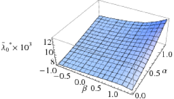
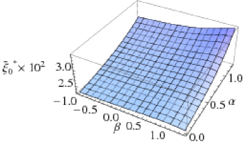
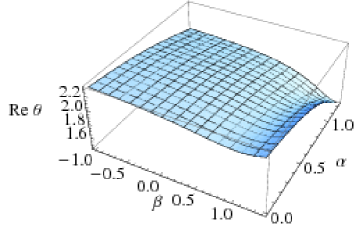
Figure 1: The gauge dependence of GMFP and critical exponents in $d=4$. For convenience of depicting the values in plot, we have rescaled $\tilde{\lambda}^{*}_{0}$ and $\tilde{\xi}^{*}_{0}$ by $1000$ and $100$ respectively.

IV.2 The GMFP in other Dimensions

We now look for the GMFP in other dimensions. For any $d>2$, in De-donder gauge, the FP equation for $\tilde{\lambda}_{0}$ and $\tilde{\xi}_{0}$ is given by,

$$2d\tilde{\lambda}_{0}+\frac{(3d-2)\tilde{\lambda}_{0}+(d-2)(d^{2}+d-1)\tilde{\xi}_{0}}{(4\pi)^{d/2}\Gamma\left(2+\frac{d}{2}\right)(\tilde{\lambda}_{0}-\tilde{\xi}_{0})} = 0\,\ ,$$ (67)

$$\frac{A\,\tilde{\lambda}_{0}^{2}+B\,\tilde{\lambda}_{0}\tilde{\xi}_{0}+C\,\tilde{\xi}_{0}^{2}}{(\tilde{\lambda}_{0}-\tilde{\xi}_{0})}+D\,(\tilde{\lambda}_{0}-\tilde{\xi}_{0}) = 0\,\ ,$$ (68)

where

$$A = -(d-1)(d^{3}+2d^{2}+36d+24)\,\ ,$$

$$B = -(d-1)(d^{5}-17d^{3}-38d^{2}-96d-48)\,\ ,$$

$$C = (d^{6}-13d^{5}+32d^{4}-104d^{3}+72d^{2}+36d+24)\,\ ,$$

$$D = 24d(d-1)(d-2)(4\pi)^{d/2}\Gamma\left(2+\frac{d}{2}\right)\,.$$ (69)

Solving these equations we find that in other dimensions, it is possible to have more than one real solution. But when we plot all the real the solutions against various $d$ in a graph, we notice that not all solutions exist in all dimensions. Only one solution exists in all dimensions, and is continuous in $d$. Besides, the ones which don’t exist in all dimensions, have large critical exponents and are probably unphysical. In Fig.2 we plot the position of the GMFP for $2<d\leq 11$, both in terms of $\tilde{\lambda}_{0}$ and $\tilde{\xi}_{0}$ and of the more familiar dimensionless cosmological constant and Newton constant

$$\tilde{\lambda}_{0}=\frac{2\tilde{\Lambda}}{16\pi\tilde{G}}\ ;\qquad\tilde{\xi}_{0}=\frac{1}{16\pi\tilde{G}}\ .$$ (70)

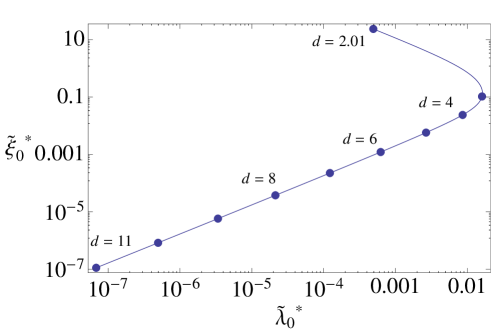
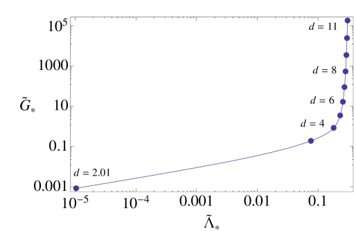
Figure 2: In the first graph we plot the GMFP $\tilde{\lambda}^{*}_{0}$ and $\tilde{\xi}^{*}_{0}$ in various dimensions. In the second plot we calculate the corresponding FP values of the cosmological constant $\tilde{\Lambda}^{*}$ and Newton’s constant $\tilde{G}^{*}$ in various dimensions.

After having found the GMFP in various dimensions, we set to calculate their critical exponents. In arbitrary dimensions, the various blocks of the stability matrix obey eq. (31). We plot the critical exponents of $M_{00}$ for various dimensions.

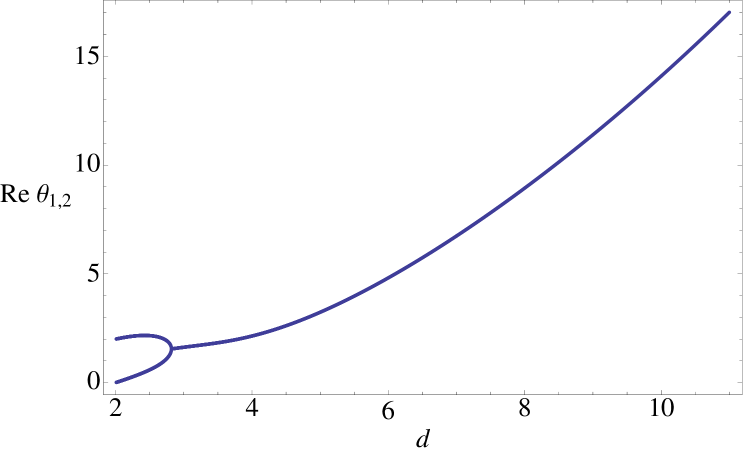
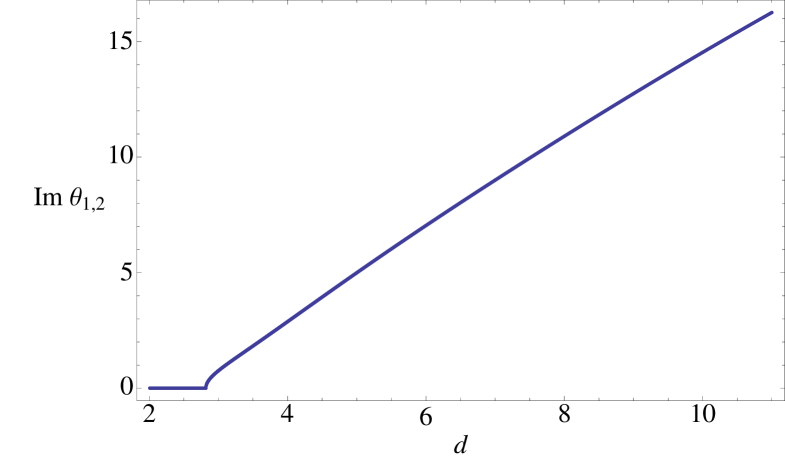
Figure 3: Critical exponents at the GMFP in various dimensions. The left panel shows the real part of the critical exponents, the right panel shows the imaginary part of the critical exponents. We note that below $d=2.8$ the critical exponents becomes real.

From the graph Fig. (3) we note that around $d=2.8$ there is bifurcation. Below $d<2.8$ the critical exponents are no more complex.

A summary of the properties of the GMFP in various dimensions is given in table (1).

$d$	$\tilde{\lambda}^{*}_{0}$	$\tilde{\xi}^{*}_{0}$	$\tilde{\Lambda}^{*}$	$\tilde{G}^{*}$	$\theta_{1}$	$\theta_{2}$
2.001	4.968 $\times 10^{-5}$	2.386 $\times 10^{2}$	1.041 $\times 10^{-7}$	8.339 $\times 10^{-5}$	2.001	0.001
3	1.605 $\times 10^{-2}$	1.047 $\times 10^{-1}$	7.666 $\times 10^{-2}$	1.900 $\times 10^{-1}$	1.627 + 0.754 $i$	1.627 - 0.754 $i$
4	8.620 $\times 10^{-3}$	2.375 $\times 10^{-2}$	1.814 $\times 10^{-1}$	8.375 $\times 10^{-1}$	2.143 + 2.879 $i$	2.143 - 2.879 $i$
5	2.669 $\times 10^{-3}$	5.744 $\times 10^{-3}$	2.323 $\times 10^{-1}$	3.463	3.236 + 4.996 $i$	3.236 - 4.996 $i$
6	6.230 $\times 10^{-4}$	1.207 $\times 10^{-3}$	2.581 $\times 10^{-1}$	1.648 $\times 10$	4.818 + 7.039 $i$	4.818 - 7.039 $i$
7	1.225 $\times 10^{-4}$	2.235 $\times 10^{-4}$	2.740 $\times 10^{-1}$	8.900 $\times 10$	6.744 + 9.004 $i$	6.744 - 9.004 $i$
8	2.133 $\times 10^{-5}$	3.738 $\times 10^{-5}$	2.853 $\times 10^{-1}$	5.322 $\times 10^{2}$	8.945 + 10.904 $i$	8.945 - 10.904 $i$
9	3.380 $\times 10^{-6}$	5.747 $\times 10^{-6}$	2.941 $\times 10^{-1}$	3.462 $\times 10^{3}$	11.396 + 12.748 $i$	11.396 - 12.748 $i$
10	4.960 $\times 10^{-7}$	8.228 $\times 10^{-7}$	3.014 $\times 10^{-1}$	2.418 $\times 10^{4}$	14.089 + 14.537 $i$	14.089 - 14.537 $i$
11	6.817 $\times 10^{-8}$	1.107 $\times 10^{-7}$	3.079 $\times 10^{-1}$	1.797 $\times 10^{5}$	17.025 + 16.261 $i$	17.025 - 16.261 $i$

Table 1: Position of GMFP and critical exponents for various dimensions.

Notice that for all the dimensions considered, the real part of the critical exponents is greater than $d-2$ and less than $2(d-2)$. As a result, in all these cases there are exactly two pairs of complex conjugate critical exponents with positive real part, i.e. four relevant directions.

Finally we studied the gauge dependence in different dimensions in the same wasy as we did in $d=4$, for example in $d=6$ we obtain the graphs shown in Fig. (4).

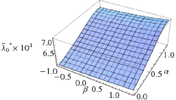
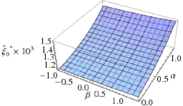
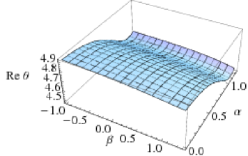
Figure 4: The gauge dependence of GMFP and critical exponents in $d=6$. For convenience of depicting the values in plot, we have rescaled $\tilde{\lambda}^{*}_{0}$ and $\tilde{\xi}^{*}_{0}$ by $10^{4}$ and $10^{3}$ respectively.

V Other Non trivial Fixed Points

Having discussed the existence and properties of the GMFP, we can ask ourselves whether there exist other FP where the scalar field has nontrivial self-interactions. We look for (truncated) polynomial FP potentials of the form

$$\tilde{V}(\tilde{\phi}^{2})=\sum_{n=0}^{a}\tilde{\lambda}_{2n}\,\tilde{\phi}^{2n}\ ;\qquad\tilde{F}(\tilde{\phi}^{2})=\sum_{n=0}^{b}\tilde{\xi}_{2n}\,\tilde{\phi}^{2n}\,.$$ (71)

with finite $a\geq 1$, $b\geq 0$. Such potentials are known not to exist in a pure scalar theory in four dimensions hhm , so we consider it unlikely that they exist in the presence of gravity, In fact the outcome of our numerical searches is that no such FP’s appear to exist in dimensions 4, 5 and 6. (Some FP do appear in certain truncations but not in others, so they are likely to be just truncation artifacts.)

The situation is somewhat different in three dimensions. We know that pure scalar theory in $d=3$ has the Wilson-Fisher FP wf . This FP can be seen in our calculations by taking the limit $\tilde{G}\to 0$ (where Newton’s constant $G$ is related to $\xi_{0}=1/16\pi G$) and $\tilde{\lambda}_{0}\to 0$, in which case gravity decouples. Solving the FP equations of the scalar field in the LPA, truncated to order $\phi^{4}$, one gets $\tilde{\lambda}^{*}_{2}=-0.0385$ and $\tilde{\lambda}^{*}_{4}=0.3234$, with critical exponents $\theta_{1}=1.843$ and $\theta_{2}=-1.176$. (These are not very good values, but we quote them here for the sake of comparison with what we find in the presence of gravity.) The FP persists when one goes to higher truncations.

One wonders whether there exists a “gravitationally dressed” Wilson-Fisher FP, with nonvanishing $\tilde{G}$, namely a FP where gravity and the scalar simultaneously have nontrivial interactions. Again in certain truncations one finds various FPs which turn out to be truncation artifacts. There seems however to exist one genuine FP: we find it in all truncations where $a\geq b$, and it has very similar properties in all truncations. To explore its properties we have looked in two directions: increasing simultaneously $a$ and $b$, or keeping $b=0$ and increasing $a$.

$(a,b)$	$\tilde{\lambda}^{*}_{0}$	$\tilde{\lambda}^{*}_{2}$	$\tilde{\lambda}^{*}_{4}$	$\tilde{\lambda}^{*}_{6}$	$\tilde{\lambda}^{*}_{8}$	$\tilde{\xi}^{*}_{0}$	$\tilde{\xi}^{*}_{2}$	$\tilde{\xi}^{*}_{4}$	$\tilde{\xi}^{*}_{6}$	$\tilde{\xi}^{*}_{8}$
(2,1)	0.0196	-0.1646	-0.1595			0.1088	-0.03108
(3,1)	0.01994	-0.1758	-0.1958	-0.2796		0.1096	-0.03810
(4,1)	0.02002	-0.1783	-0.2041	-0.3466	-0.5579	0.1098	-0.03969
(2,2)	0.01894	-0.1408	-0.1241			0.1071	-0.01122	0.04297
(3,2)	0.01971	-0.1680	-0.1848	-0.2879		0.1089	-0.03131	0.01731
(4,2)	0.01988	-0.1735	-0.1975	-0.3544	-0.5687	0.1093	-0.03542	0.01121
(3,3)	0.01911	-0.1469	-0.1469	-0.1935		0.1074	-0.01420	0.05017	0.1617
(4,3)	0.01953	-0.1618	-0.1768	-0.3083	-0.6569	0.1084	-0.02571	0.03197	0.1102
(4,4)	0.01923	-0.1512	-0.1572	-0.2496	-0.4911	0.1077	-0.01728	0.04732	0.1765	0.3868

Table 2: Position of Nontrivial FP in $d=3$ for various truncations.

$(a,b)$	$\theta_{1}^{\prime}$	$\theta_{1}^{\prime\prime}$	$\theta_{3}$	$\theta_{4}$	$\theta_{5}$	$\theta_{6}$	$\theta_{7}$
(2,1)	1.648	0.592	-0.956	-3.902	-13.46
(3,1)	1.650	0.554	-1.079	-3.776	-11.20	-29.397
(4,1)	1.650	0.543	-1.105	-3.673	-10.02	-24.01	-49.31
$(a,b)$	$\theta_{1}^{\prime}$	$\theta_{1}^{\prime\prime}$	$\theta_{2}^{\prime}$	$\theta_{2}^{\prime\prime}$	$\theta_{5}$	$\theta_{6}$	$\theta_{7}$	$\theta_{8}$
(2,2)	1.649	0.656	-7.979	1.261	-0.559	-3.192
(3,2)	1.652	0.589	-7.933	3.909	-0.835	-3.578	-27.67
(4,2)	1.652	0.570	-7.635	4.083	-0.898	-3.626	-22.64	- 47.78
$(a,b)$	$\theta_{1}^{\prime}$	$\theta_{1}^{\prime\prime}$	$\theta_{2}^{\prime}$	$\theta_{2}^{\prime\prime}$	$\theta_{3}^{\prime}$	$\theta_{3}^{\prime\prime}$	$\theta_{7}$	$\theta_{8}$	$\theta_{9}$
(3,3)	1.649	0.641	-6.703	2.097	-14.12	8.990	-0.512	-2.991
(4,3)	1.651	0.603	-6.448	3.343	-13.94	10.91	-0.657	-3.287	-42.28
$(a,b)$	$\theta_{1}^{\prime}$	$\theta_{1}^{\prime\prime}$	$\theta_{2}^{\prime}$	$\theta_{2}^{\prime\prime}$	$\theta_{3}^{\prime}$	$\theta_{3}^{\prime\prime}$	$\theta_{3}^{\prime}$	$\theta_{3}^{\prime\prime}$	$\theta_{9}$	$\theta_{10}$
(4,4)	1.650	0.630	-5.958	2.008	-12.88	7.966	-20.07	19.03	-0.513	-2.977

Table 3: Critical exponents at Non trivial FP in $d=3$ for various truncations. When the critical exponents are complex we write them in the form $\theta_{\ell}^{\prime}\pm i\theta_{\ell}^{\prime\prime}$

Tables (2) and (3) give the position and critical exponents of this FP for $a\geq b$ and $b\leq 4$. One notices that $\tilde{\lambda}^{*}_{2n}<0$ for all $n>0$ in the table. It is computationally demanding to continue in this direction, so to have some indication on the sign of $\tilde{\lambda}^{*}_{2n}$ for higher $n$ we considered a simple truncation where $\tilde{F}$ is constant, i.e. $\tilde{\xi}_{n}=0$ for $n>0$. In this case we could push the truncation up to $a=8$. The results are given in tables (4) and (5). One sees that the coefficients of the potential are indeed all negative.

$(a,b)$	$\tilde{\lambda}^{*}_{0}$	$\tilde{\lambda}^{*}_{2}$	$\tilde{\lambda}^{*}_{4}$	$\tilde{\lambda}^{*}_{6}$	$\tilde{\lambda}^{*}_{8}$	$\tilde{\lambda}^{*}_{10}$	$\tilde{\lambda}^{*}_{12}$	$\tilde{\lambda}^{*}_{14}$	$\tilde{\lambda}^{*}_{16}$	$\tilde{\xi}^{*}_{0}$
(1,0)	0.01813	-0.1088								0.1060
(2,0)	0.01880	-0.1343	-0.1561							0.1065
(3,0)	0.01894	-0.1395	-0.1942	-0.2633						0.1066
(4,0)	0.01898	-0.1407	-0.2032	-0.3284	-0.4998					0.1066
(5,0)	0.01899	-0.1410	-0.2053	-0.3437	-0.6182	-0.9604				0.1066
(6,0)	0.01899	-0.1411	-0.2058	-0.3472	-0.6452	-1.180	-1.826			0.1066
(7,0)	0.01899	-0.1411	-0.2059	-0.3479	-0.6511	-1.228	-2.229	-3.380		0.1066
(8,0)	0.01899	-0.1411	-0.2059	-0.3481	-0.6524	-1.238	-2.313	-4.091	-5.977	0.1066

Table 4: Position of Nontrivial FP in $d=3$ for other truncations.

$(a,b)$	$\theta_{1}^{\prime}$	$\theta_{1}^{\prime\prime}$	$\theta_{3}$	$\theta_{4}$	$\theta_{5}$	$\theta_{6}$	$\theta_{7}$	$\theta_{8}$	$\theta_{9}$	$\theta_{10}$
(1,0)	1.659	0.753	-1.699
(2,0)	1.675	0.745	-1.594	-10.59
(3,0)	1.679	0.742	-1.485	-8.384	-22.41
(4,0)	1.68	0.741	-1.434	-7.341	-18.19	-36.96
(5,0)	1.68	0.741	-1.414	-6.84	-15.93	-31.12	-54.10
(6,0)	1.68	0.741	-1.407	-6.609	-14.70	-27.47	-47.25	-73.60
(7,0)	1.68	0.740	-1.405	-6.509	-14.02	-25.287	-42.062	-66.663	-95.172
(8,0)	1.68	0.740	-1.405	-6.469	-13.67	-23.94	-38.77	-59.72	-89.58	-118.4

Table 5: Critical Exponents at Non trivial FP in $d=3$ for other truncations.

Furthermore, the coefficients grow in absolute value, so the series for $V$ has a very small radius of convergence. This is similar to the situation discussed in hhm , making the FP unphysical. So we conclude that also in three dimensions there is probably no physically viable FP besides the GMFP.

VI Conclusions

The results of this paper confirm and extend the findings of Perini2 . The GMFP is found to exist also in other dimensions and in other gauges, and (with the possible exception of $d=3$) there does not seem to be other FP’s with nontrivial scalar self-interactions. In four dimensions this agrees with the findings of hhm .

These results may be applied in various settings. The beta functions given in Appendix A contain the full dependence on the dimensionless parameters $\tilde{\lambda}_{0}$, $\tilde{\xi}_{0}$, $\tilde{\lambda}_{2}$, $\tilde{\xi}_{2}$, $\tilde{\lambda}_{4}$, without making any assumption on the value of these couplings (which in the case of the first three means the ratio between the dimensionful couplings $\lambda_{0}$, $\xi_{0}$, $\lambda_{2}$ and the RG scale $k$). In particular, threshold effects are taken into account by the denominators $1+2\tilde{\lambda}_{2}$ and $\tilde{\xi}_{0}-\tilde{\lambda}_{0}$. One can easily recognize among various terms the ones that are obtained in perturbative approximations, but we emphasize that the derivation of these beta functions using the FRGE does not require that the couplings be small.

The most natural application of these results seems to be in the context of early cosmology, where a scalar field is used to drive inflation. In an asymptotic safety context, it would be attractive to obtain inflation as a result of FP behavior along the lines of Reutercosmology . In fact the energy scale involved is sufficiently high that one may expect quantum gravity effects to play some role. Alternatively, it would also be of interest to apply the flow equations derived here to the scalar tensor theory, e.g. to improve the results of higgsflaton .

According to various speculations, quantum effects may play a role also on very large scales, and then again the RG flow of scalar-tensor theory could become relevant. In this connection we recall that scalar-tensor theories of a different type also arise in the conformal reduction of pure gravity, and have been studied from the FRGE point of view in Weyer ; crehroberto .

We have mentioned in the Introduction that scalar-tensor theories can be reformulated classically also as pure gravity theories with $f(R)$ type actions, and one may wonder whether there is a relation also between their RG flows. In particular one could ask whether the FP that was found in CPR ; MachSau has a counterpart in the equivalent scalar-tensor theory. At first sight one would think that this is not the case, because the choice of cutoff breaks the classical equivalence between these theories. Still, this point deserves a more detailed investigation.

Another direction for research is the inclusion of other matter fields. As discussed in the introduction, if asymptotic safety is indeed the answer to the UV issues of quantum field theory, then it will not be enough to establish asymptotic safety of gravity: one will have to establish asymptotic safety for a theory including gravity as well as all the fields that occur in the standard model, and perhaps even other ones that have not yet been discovered. Ideally one would like to have a unified theory of all interactions including gravity, perhaps a GraviGUT along the lines of nesti . More humbly one could start by studying the effect of gravity on the interactions of the standard model or GUTs. Fortunately, for some important parts of the standard model it is already known that an UV Gaussian FP exists, so the question is whether the coupling to gravity, or some other mechanism, can cure the bad behavior of QED and of the Higgs sector. That this might happen had been speculated long ago fradkintseytlin ; see also buchbinder for some detailed calculations. It seem that the existence of a GMFP for all matter interactions would be the simplest solution to this issue. In this picture of asymptotic safety, gravity would be the only effective interaction at sufficiently high scale. The possibility of asymptotic safety in a nonlinearly realized scalar sector has been discussed in coza . Aside from scalar tensor theories, the effect of gravity has been studied in Wilczek for gauge couplings and Zanusso for Yukawa couplings.

Appendix A Explicit beta functions

In section II.B we have presented equations which in principle determine the beta functionals for $V$ and $F$ in $d=4$ and in the gauge $\alpha=0$ and $\beta=1$. At one loop the beta functionals can be immediately read off from there, but if one wants to get the “improved” beta functionals (meaning that no approximation is made beyond the truncation), then the system is too complicated to be solved. It can be solved if we assume that $V$ and $F$ are finite polynomials. We give here a set of linear equations that determine the beta functions in a five coupling truncation, including $\lambda_{0}$, $\xi_{0}$, $\lambda_{2}$, $\xi_{2}$, $\lambda_{4}$. These equations can be easily solved using algebraic manipulation software. This exercise will also enable us to compare with familiar one loop results. These beta functions had been written previously in Perini2 , but since there we had left the cutoff generic, it was not possible to compute the integrals over momenta, which are contained in the expressions $Q_{2}$ and $Q_{1}$. Here the integrals have already been performed, using an optimized cutoff Litim:cf , so the beta functions are in closed form and completely explicit. We use the notation $\eta=\frac{\partial_{t}\xi_{0}}{\xi_{0}}=\frac{\partial_{t}\tilde{\xi}_{0}}{\tilde{\xi}_{0}}+2$.

$$\partial_{t}\tilde{\lambda}_{0}= -4\tilde{\lambda}_{0}+\frac{1}{32\pi^{2}}\left[2+\frac{1}{1+2\tilde{\lambda}_{2}}+\frac{6\tilde{\lambda}_{0}}{\tilde{\xi}_{0}-\tilde{\lambda}_{0}}\right]+\frac{\eta}{96\pi^{2}}\frac{5\tilde{\xi}_{0}-2\tilde{\lambda}_{0}}{\tilde{\xi}_{0}-\tilde{\lambda}_{0}},$$ (72)

$$\partial_{t}\tilde{\xi}_{0}= -2\tilde{\xi}_{0}+\frac{1}{384\pi^{2}}\left[25-\frac{4}{1+2\tilde{\lambda}_{2}}-\frac{24\tilde{\xi}_{2}}{(1+2\tilde{\lambda}_{2})^{2}}+\frac{8\tilde{\xi}_{0}(7\tilde{\xi}_{0}-2\tilde{\lambda}_{0})}{(\tilde{\xi}_{0}-\tilde{\lambda}_{0})^{2}}\right]+\frac{\eta}{1152\pi^{2}}\frac{17\tilde{\xi}_{0}^{2}+18\tilde{\xi}_{0}\tilde{\lambda}_{0}-15\tilde{\lambda}_{0}^{2}}{(\tilde{\xi}_{0}-\tilde{\lambda}_{0})^{2}},$$ (73)

$$\partial_{t}\tilde{\lambda}_{2}= -2\tilde{\lambda}_{2}+\frac{1}{48\pi^{2}}\Biggl{[}\frac{9\tilde{\lambda}_{0}(1+2\tilde{\xi}_{2})}{2(\tilde{\xi}_{0}-\tilde{\lambda}_{0})^{2}}-\frac{9(2\tilde{\lambda}_{0}-\tilde{\xi}_{0})(1+2\tilde{\xi}_{2})^{2}}{2(1+2\tilde{\lambda}_{2})(\tilde{\xi}_{0}-\tilde{\lambda}_{0})^{2}}-\frac{9(1+2\tilde{\xi}_{2})^{2}}{2(1+2\tilde{\lambda}_{2})^{2}(\tilde{\xi}_{0}-\tilde{\lambda}_{0})}-\frac{18\tilde{\lambda}_{4}}{(1+2\tilde{\lambda}_{2})^{2}}\Biggr{]}$$

$$+\frac{\eta}{96\pi^{2}}\left[-\frac{2\tilde{\xi}_{2}}{\tilde{\xi}_{0}}+\frac{3\tilde{\xi}_{0}(1+2\tilde{\xi}_{2})}{2(\tilde{\xi}_{0}-\tilde{\lambda}_{0})^{2}}-\frac{3\tilde{\xi}_{0}(1+2\tilde{\xi}_{2})^{2}}{2(1+2\tilde{\lambda}_{2})(\tilde{\xi}_{0}-\tilde{\lambda}_{0})^{2}}\right]+\frac{1}{96\pi^{2}}\frac{\partial_{t}\tilde{\xi}_{2}}{\tilde{\xi}_{0}}\left[2-\frac{3\tilde{\xi}_{0}}{\tilde{\xi}_{0}-\tilde{\lambda}_{0}}+\frac{6\tilde{\xi}_{0}(1+2\tilde{\xi}_{2})}{(1+2\tilde{\lambda}_{2})(\tilde{\xi}_{0}-\tilde{\lambda}_{0})}\right],$$ (74)

$$\partial_{t}\tilde{\xi}_{2}= \frac{1}{576\pi^{2}}\Biggl{[}\frac{1+2\tilde{\lambda}_{2}}{\tilde{\xi}_{0}-\tilde{\lambda}_{0}}\left(9+\frac{39\tilde{\xi}_{0}}{\tilde{\xi}_{0}-\tilde{\lambda}_{0}}+\frac{60\tilde{\xi}_{0}^{2}}{(\tilde{\xi}_{0}-\tilde{\lambda}_{0})^{2}}\right)+\frac{3(3+32\tilde{\xi}_{2})}{\tilde{\xi}_{0}-\tilde{\lambda}_{0}}-\frac{6\tilde{\xi}_{0}(11+2\tilde{\xi}_{2})}{(\tilde{\xi}_{0}-\tilde{\lambda}_{0})^{2}}-\frac{60\tilde{\xi}_{0}^{2}(1+2\tilde{\xi}_{2})}{(\tilde{\xi}_{0}-\tilde{\lambda}_{0})^{3}}$$

$$+\frac{216\tilde{\xi}_{2}(1+2\tilde{\xi}_{2})^{2}}{(1+2\tilde{\lambda}_{2})^{3}(\tilde{\xi}_{0}-\tilde{\lambda}_{0})}+\frac{9[\tilde{\lambda}_{0}(5-2\tilde{\xi}_{2})-2\tilde{\xi}_{0}(1+2\tilde{\xi}_{2})](1+2\tilde{\xi}_{2})}{(1+2\tilde{\lambda}_{2})(\tilde{\xi}_{0}-\tilde{\lambda}_{0})^{2}}+\frac{27(1+2\tilde{\xi}_{2})(1-10\tilde{\xi}_{2}-16\tilde{\xi}_{2}^{2})}{(1+2\tilde{\lambda}_{2})^{2}(\tilde{\xi}_{0}-\tilde{\lambda}_{0})}$$

$$+\frac{108\tilde{\xi}_{0}\tilde{\xi}_{2}(1+2\tilde{\xi}_{2})^{2}}{(1+2\tilde{\lambda}_{2})^{2}(\tilde{\xi}_{0}-\tilde{\lambda}_{0})^{2}}+\frac{72\tilde{\lambda}_{4}}{(1+2\tilde{\lambda}_{2})^{2}}\frac{1+12\tilde{\xi}_{2}+2\tilde{\lambda}_{2}}{1+2\tilde{\lambda}_{2}}\Biggr{]}+\frac{\eta}{1152\pi^{2}}\Biggl{[}\frac{1+2\tilde{\lambda}_{2}}{\tilde{\xi}_{0}-\tilde{\lambda}_{0}}\left(3+\frac{18\tilde{\xi}_{0}}{\tilde{\xi}_{0}-\tilde{\lambda}_{0}}+\frac{20\tilde{\xi}_{0}^{2}}{(\tilde{\xi}_{0}-\tilde{\lambda}_{0})^{2}}\right)$$

$$+\frac{15\tilde{\xi}_{2}}{\tilde{\xi}_{0}}-\frac{6(1+\tilde{\xi}_{2})}{\tilde{\xi}_{0}-\tilde{\lambda}_{0}}-\frac{10\tilde{\xi}_{0}(3+4\tilde{\xi}_{2})}{(\tilde{\xi}_{0}-\tilde{\lambda}_{0})^{2}}-\frac{20\tilde{\xi}_{0}^{2}(1+2\tilde{\xi}_{2})}{(\tilde{\xi}_{0}-\tilde{\lambda}_{0})^{3}}-\frac{3[\tilde{\lambda}_{0}-\tilde{\xi}_{0}(5-4\tilde{\xi}_{2})](1+2\tilde{\xi}_{2})}{(1+2\tilde{\lambda}_{2})(\tilde{\xi}_{0}-\tilde{\lambda}_{0})^{2}}+\frac{36\tilde{\xi}_{0}\tilde{\xi}_{2}(1+2\tilde{\xi}_{2})^{2}}{(1+2\tilde{\lambda}_{2})^{2}(\tilde{\xi}_{0}-\tilde{\lambda}_{0})^{2}}\Biggr{]}$$

$$+\frac{1}{1152\pi^{2}}\frac{\partial_{t}\tilde{\xi}_{2}}{\tilde{\xi}_{0}}\left[-15+\frac{54\tilde{\xi}_{0}}{\tilde{\xi}_{0}-\tilde{\lambda}_{0}}+\frac{20\tilde{\xi}_{0}^{2}}{(\tilde{\xi}_{0}-\tilde{\lambda}_{0})^{2}}-\frac{6\tilde{\xi}_{0}(7+2\tilde{\xi}_{2})}{(1+2\tilde{\lambda}_{2})(\tilde{\xi}_{0}-\tilde{\lambda}_{0})}-\frac{144\tilde{\xi}_{0}\tilde{\xi}_{2}(1+2\tilde{\xi}_{2})}{(1+2\tilde{\lambda}_{2})^{2}(\tilde{\xi}_{0}-\tilde{\lambda}_{0})}\right],$$ (75)

$$\partial_{t}\tilde{\lambda}_{4}= \frac{1}{48\pi^{2}}\Biggl{[}\frac{9}{4(\tilde{\xi}_{0}-\tilde{\lambda}_{0})^{2}}\Biggl{(}5(1+2\tilde{\lambda}_{2})(1+4\tilde{\xi}_{2})-(1+2\tilde{\xi}_{2})(21+62\tilde{\xi}_{2})+\frac{33(1+2\tilde{\xi}_{2})^{3}}{1+2\tilde{\lambda}_{2}}$$

$$-\frac{(1+2\tilde{\xi}_{2})^{3}(23+24\tilde{\xi}_{2})}{(1+2\tilde{\lambda}_{2})^{2}}+\frac{6(1+2\tilde{\xi}_{2})^{4}}{(1+2\tilde{\lambda}_{2})^{3}}\Biggr{)}+\frac{9\tilde{\xi}_{0}(\tilde{\xi}_{2}-\tilde{\lambda}_{2})^{2}}{(\tilde{\xi}_{0}-\tilde{\lambda}_{0})^{3}}\left(6\frac{(1+2\tilde{\xi}_{2})^{2}}{(1+2\tilde{\lambda}_{2})^{2}}-10\frac{1+2\tilde{\xi}_{2}}{1+2\tilde{\lambda}_{2}}+5\right)$$

$$-\frac{72\tilde{\lambda}_{2}\tilde{\lambda}_{4}(1+2\tilde{\xi}_{2})(1-4\tilde{\lambda}_{2}+6\tilde{\xi}_{2})}{(\tilde{\xi}_{0}-\tilde{\lambda}_{0})(1+2\tilde{\lambda}_{2})^{3}}+\frac{9\tilde{\xi}_{0}\tilde{\lambda}_{4}}{(\tilde{\xi}_{0}-\tilde{\lambda}_{0})^{2}}\left(6\frac{(1+2\tilde{\xi}_{2})^{2}}{(1+2\tilde{\lambda}_{2})^{2}}-8\frac{1+2\tilde{\xi}_{2}}{1+2\tilde{\lambda}_{2}}+3\right)+\frac{216\tilde{\lambda}_{4}^{2}}{(1+2\tilde{\lambda}_{2})^{3}}\Biggr{]}$$

$$+\frac{\eta}{96\pi^{2}}\Biggl{[}\frac{2\tilde{\xi}_{2}^{2}}{\tilde{\xi}_{0}^{2}}+\frac{3\tilde{\xi}_{0}(\tilde{\xi}_{2}-\tilde{\lambda}_{2})^{2}}{(\tilde{\xi}_{0}-\tilde{\lambda}_{0})^{3}}\left(6\frac{(1+2\tilde{\xi}_{2})^{2}}{(1+2\tilde{\lambda}_{2})^{2}}-10\frac{1+2\tilde{\xi}_{2}}{1+2\tilde{\lambda}_{2}}+5\right)+\frac{3\tilde{\xi}_{0}\tilde{\lambda}_{4}}{(\tilde{\xi}_{0}-\tilde{\lambda}_{0})^{2}}\left(6\frac{(1+2\tilde{\xi}_{2})^{2}}{(1+2\tilde{\lambda}_{2})^{2}}-8\frac{1+2\tilde{\xi}_{2}}{1+2\tilde{\lambda}_{2}}+3\right)\Biggr{]}$$

$$+\frac{1}{96\pi^{2}}\frac{\partial_{t}\tilde{\xi}_{2}}{\tilde{\xi}_{0}}\Biggl{[}-\frac{2\tilde{\xi}_{2}}{\tilde{\xi}_{0}}-\frac{3\tilde{\xi}_{0}(\tilde{\xi}_{2}-\tilde{\lambda}_{2})}{(\tilde{\xi}_{0}-\tilde{\lambda}_{0})^{2}}\left(12\frac{(1+2\tilde{\xi}_{2})^{2}}{(1+2\tilde{\lambda}_{2})^{2}}-21\frac{1+2\tilde{\xi}_{2}}{1+2\tilde{\lambda}_{2}}+10\right)-\frac{24\tilde{\xi}_{0}\tilde{\lambda}_{4}(1-4\tilde{\lambda}_{2}+6\tilde{\xi}_{2})}{(1+2\tilde{\lambda}_{2})^{2}(\tilde{\xi}_{0}-\tilde{\lambda}_{0})}\Biggr{]}\ .$$ (76)

If one neglects the terms involving $\eta$ and $\partial_{t}\tilde{\xi}_{2}$ in the r.h.s., then the remaining terms are the one loop beta functions for the couplings. One can recognize among them some familiar terms. The term containing $-18\tilde{\lambda}_{4}$ in the first line of eq. (A) and the term containing $216\tilde{\lambda}_{4}^{2}$ in the third line of eq. (A) are the familiar beta functions of the mass and of the coupling in $\phi^{4}$ theory in flat space. The term containing $72\lambda_{4}(1+12\xi_{2})$ in the third line of eq. (A) is also known from earlier calculations buchbinder ; higgsflaton .

Notice the ubiquitous appearance of the factors $1/(1+2\tilde{\lambda}_{2})$, which represent threshold effects for the contributions of scalar loops: for $k^{2}\gg\lambda_{2}$, $\tilde{\lambda}_{2}\ll 1$ and the denominator can be approximated by $1$, whereas for $k^{2}\ll\lambda_{2}$, $\tilde{\lambda}_{2}\gg 1$ and the term is suppressed. The denominators $\tilde{\xi}_{0}-\tilde{\lambda}_{0}$ have a somewhat similar effect. When written in terms of the more familiar variables $\Lambda$ and $G$ defined in eq. (70), they give rise to denominators $(1-2\tilde{\Lambda})$. These can be approximated by $1$ when $\Lambda\ll k^{2}$ but they vanish when the dimensionless cosmological constant $\tilde{\Lambda}$ tends to $1/2$, corresponding to an infrared singularity in the RG trajectories. This is well documented in the literature.

The term proportional to $9\tilde{\xi}_{0}\tilde{\lambda}_{4}$ in the third line of eq. (A) is the leading gravitational correction (of order $\tilde{G}$) to the running of the scalar self coupling. Note that for small $\tilde{\lambda}_{0}$, $\tilde{\lambda}_{2}$ and $\tilde{\xi}_{2}$, the denominator and the bracket to its right can be expanded as $1+O(\tilde{\lambda}_{0})+O(\tilde{\lambda}_{2})+O(\tilde{\xi}_{2})$. The order of magnitude and sign of this term agree with the calculations done in GrigPerc , in the gauge $\alpha=0$. One should not expect the results to agree exactly, because this term is gauge dependent and the calculation was done in a different gauge (namely $\beta=-1$). Notice that this term is proportional to $\tilde{\lambda}_{4}$, thus when we set $\tilde{\lambda}_{4}$ to zero, the beta function for $\tilde{\lambda}_{4}$ does not get any contribution from gravity, in agreement with the general statement that minimal coupling is self consistent. We observe that the same phenomenon happens in the case of the Yukawa coupling Zanusso and of the gauge coupling Wilczek .

References

- (1) B. Whitt, Phys. Lett. B 145 (1984) 176. K. I. Maeda, Phys. Rev. D 39 (1989) 3159. G. Magnano and L. M. Sokolowski, Phys. Rev. D 50 (1994) 5039 [arXiv:gr-qc/9312008]. E. T. Tomboulis, Phys. Lett. B 389, 225 (1996) [arXiv:hep-th/9601082]. V. Faraoni, E. Gunzig and P. Nardone, Fund. Cosmic Phys. 20 (1999) 121 [arXiv:gr-qc/9811047]. T. Chiba, Phys. Lett. B 575, 1 (2003) [arXiv:astro-ph/0307338].
- (2) S. Weinberg, In General Relativity: An Einstein centenary survey, ed. S. W. Hawking and W. Israel, pp.790–831; Cambridge University Press (1979).
- (3) M. Reuter, Phys. Rev. D57, 971 (1998) [arXiv:hep-th/9605030].
- (4) D. Dou and R. Percacci, Class. Quant. Grav. 15 (1998) 3449; [arXiv:hep-th/9707239].
- (5) W. Souma, Prog. Theor. Phys. 102, 181 (1999); [arXiv:hep-th/9907027].
- (6) O. Lauscher and M. Reuter, Phys. Rev. D65, 025013 (2002); [arXiv:hep-th/0108040]; Class. Quant. Grav. 19, 483 (2002); [arXiv:hep-th/0110021]; Int. J. Mod. Phys. A 17, 993 (2002); [arXiv:hep-th/0112089]; M. Reuter and F. Saueressig, Phys. Rev. D65, 065016 (2002). [arXiv:hep-th/0110054].
- (7) O. Lauscher and M. Reuter, Phys. Rev. D 66, 025026 (2002) [arXiv:hep-th/0205062].
- (8) M. Reuter and F. Saueressig, Phys. Rev. D 66, 125001 (2002) [arXiv:hep-th/0206145]; Fortsch. Phys. 52, 650 (2004) [arXiv:hep-th/0311056].
- (9) P. Fischer and D. F. Litim, Phys. Lett. B 638 (2006) 497 [arXiv:hep-th/0602203].
- (10) M. Reuter and H. Weyer, arXiv:0801.3287 [hep-th]; Phys. Rev. D 80, 025001 (2009) [arXiv:0804.1475 [hep-th]].
- (11) A. Codello and R. Percacci, Phys.Rev.Lett. 97, 221301 (2006); e-Print: hep-th/0607128.
- (12) R. Percacci, Phys. Rev. D73, 041501(R) (2006); [arXiv:hep-th/0511177].
- (13) A. Codello, R. Percacci and C. Rahmede, Int. J. Mod. Phys. A 23 (2008) 143 [arXiv:0705.1769 [hep-th]]; Annals Phys. 324 (2009) 414 [arXiv:0805.2909 [hep-th]].
- (14) P. F. Machado and F. Saueressig, Phys. Rev. D 77, 124045 (2008) [arXiv:0712.0445 [hep-th]].
- (15) D. Benedetti, P. F. Machado and F. Saueressig, arXiv:0901.2984 [hep-th]; arXiv:0902.4630 [hep-th] and arXiv:0909.3265 [hep-th].
- (16) M. R. Niedermaier, Phys. Rev. Lett. 103, 101303 (2009).
- (17) M. Reuter and H. Weyer, Phys. Rev. D 79 (2009) 105005 and arXiv:0801.3287 [hep-th]; Gen. Rel. Grav. 41 (2009) 983 and arXiv:0903.2971 [hep-th].
- (18) E. Manrique and M. Reuter, Phys. Rev. D 79, 025008 (2009) [arXiv:0811.3888 [hep-th]]; arXiv:0907.2617 [gr-qc].
- (19) A. Eichhorn, H. Gies and M. M. Scherer, arXiv:0907.1828 [hep-th].
- (20) Max Niedermaier and Martin Reuter, Living Rev. Relativity 9, (2006), 5. M. Niedermaier, Class. Quant. Grav. 24 (2007) R171 [arXiv:gr-qc/0610018]. R. Percacci, “Asymptotic Safety”, to appear in “Approaches to Quantum Gravity: Towards a New Understanding of Space, Time and Matter” ed. D. Oriti, Cambridge University Press; e-Print: arXiv:0709.3851 [hep-th]. D. F. Litim, arXiv:0810.3675 [hep-th].
- (21) G. ’t Hooft and M. J. G. Veltman, Annales Poincare Phys. Theor. A 20 (1974) 69; S. Deser, H.S. Tsao and P. van Nieuwenhuizen, Phys. Lett. 50B 491 (1974); Phys. Rev. D10 3337 (1974); S. Deser, and P. van Nieuwenhuizen, Phys. Rev. D10 411 (1974).
- (22) R. Percacci and D. Perini, Phys. Rev. D67, 081503(R) (2003) [arXiv:hep-th/0207033].
- (23) M. Reuter and F. Saueressig, JCAP 0509 (2005) 012 [arXiv:hep-th/0507167]; M. Reuter and F. Saueressig, JCAP 0509 (2005) 012 [arXiv:hep-th/0507167]; A. Bonanno and M. Reuter, JCAP 0708 (2007) 024 [arXiv:0706.0174 [hep-th]].
- (24) C. Wetterich, Astron. Astrophys. 301 321-328 (1995) e-Print: hep-th/9408025; Phys. Rev. Lett. 102 141303 (2009), e-Print: arXiv:0806.0741 [hep-th].
- (25) C. Wetterich, Phys. Lett. B 301, 90 (1993).
- (26) T. R. Morris, Phys. Lett. B 329 (1994) 241 [arXiv:hep-ph/9403340].
- (27) C. Bagnuls and C. Bervillier, Phys. Rept. 348 (2001) 91 [arXiv:hep-th/0002034].
- (28) J. Berges, N. Tetradis and C. Wetterich, Phys. Rept. 363 (2002) 223 [arXiv:hep-ph/0005122].
- (29) H. Gies, Phys. Rev. D 66 (2002) 025006 [arXiv:hep-th/0202207].
- (30) J. M. Pawlowski, arXiv:hep-th/0512261.
- (31) C. Bervillier, A. Juttner and D. F. Litim, Nucl. Phys. B 783, 213 (2007) [arXiv:hep-th/0701172].
- (32) T. R. Morris, Phys. Lett. B 334 (1994) 355 [arXiv:hep-th/9405190].
- (33) E.S. Fradkin and A.A. Tseytlin, Nucl. Phys. B 201 469 (1982).
- (34) L. Griguolo and R. Percacci, Phys. Rev. D 52, 5787 (1995) [arXiv:hep-th/9504092].
- (35) R. Percacci and D. Perini, Phys. Rev. D 68 (2003) 044018 [arXiv:hep-th/0304222].
- (36) D. F. Litim, Phys. Lett. B 486 (2000) 92 [arXiv:hep-th/0005245]. Phys. Rev. D 64 (2001) 105007 [arXiv:hep-th/0103195].
- (37) F.L. Bezrukov, M. Shaposhnikov, Phys. Lett. B659 703-706 (2008) arXiv: arXiv:0710.3755 [hep-th]; A. De Simone, M.P. Hertzberg, F. Wilczek, Phys. Lett. B6781-8 (2009) arXiv:0812.4946 [hep-ph]; C.P. Burgess, Hyun Min Lee, M. Trott, JHEP 0909:103 (2009) arXiv:0902.4465 [hep-ph]; T.E. Clark, Boyang Liu, S.T. Love, T. ter Veldhuis, arXiv:0906.5595 [hep-ph]; A.O. Barvinsky, A.Yu. Kamenshchik, C. Kiefer, A.A. Starobinsky, C.F. Steinwachs, arXiv:0910.1041 [hep-ph].
- (38) I. Antoniadis, P.O. Mazur and E. Mottola, Phys. Rev. Lett. 79 14-17 (1997) e-Print: astro-ph/9611208 Phys. Lett. B 444 284-292 (1998) e-Print: hep-th/9808070 New J. Phys. 9 11 (2007) e-Print: gr-qc/0612068 E. Mottola and R. Vaulin, Phys. Rev. D 74 064004 (2006) e-Print: gr-qc/0604051
- (39) P. F. Machado and R. Percacci, Phys. Rev. D 80, 024020 (2009) [arXiv:0904.2510 [hep-th]].
- (40) K. G. Wilson and M. E. Fisher, Phys. Rev. Lett. 28, 240 (1972).
- (41) G. Narain and C. Rahmede, “Renormalization Group Flow in Scalar-Tensor Theories. II”, arXiv:0911.0394[hep-th].
- (42) E. Manrique and M. Reuter, e-Print: arXiv:0907.2617 [gr-qc]
- (43) K. Halpern and K. Huang, Phys. Rev. Lett. 74 3526-3529 (1995) arXiv: hep-th/9406199; Phys. Rev. D53 3252-3259 (1996) arXiv: hep-th/9510240 Phys. Rev. Lett. 77 1659 (1966); T. R. Morris, Phys. Rev. Lett. 77, 1658 (1996) arXiv:hep-th/9601128.
- (44) K.G. Wilson, M.E. Fisher, Phys. Rev. Lett. 28 240-243 (1972).
- (45) R. Percacci, Phys. Lett. B144 37-40 (1984); Nucl. Phys.B353 271-290 (1991); F. Nesti, R. Percacci, J.Phys. A41 075405 (2008) arXiv:0706.3307 [hep-th]; arXiv:0909.4537 [hep-th]; R. Percacci arXiv:0910.5167 [hep-th].
- (46) I.L. Buchbinder, S.D. Odintsov and I.L. Shapiro, “Effective action in quantum gravity”, IOPP Publishing, Bristol (1992).
- (47) A. Codello and R. Percacci, Phys. Lett. B672 280-283 (2009); arXiv:0810.0715 [hep-th]; R. Percacci and O. Zanusso, arXiv:0910.0851 [hep-th]
- (48) S. P. Robinson and F. Wilczek, Phys. Rev. Lett. 96, 231601 (2006) [arXiv:hep-th/0509050]. J.E. Daum, U. Harst, M. Reuter, arXiv:0910.4938 [hep-th]
- (49) O. Zanusso, L. Zambelli, G. P. Vacca and R. Percacci, arXiv:0904.0938 [hep-th].