Spin-Density-Wave and Asymmetry of Coherence Peaks in iron-Pnictide Superconductors from a two-orbital model

Abstract

We study theoretically the coexistence of the spin-density-wave (SDW) and superconductivity in electron-doped iron-pnictide superconductors based on the two orbital model and Bogoliubov-de Gennes equations. The phase diagram is mapped out and the evolution of the Fermi surface as the doping varies is presented. The local density of states has also been calculated from low to high doping. We show that the strength of the superconducting coherence peak at the positive energy gets enhanced and the one at the negative energy is suppressed by the SDW order in the underdoped region. Several features of our results are in good agreement with the experiments.

The discovery of the iron-based superconducting (SC) materials kam has attracted much attention. These materials share some common features of the high-T_c cuprates mik , with high transition temperature, layered system and similar phase diagram. The parent compounds are with spin-density-wave (SDW) or antiferromagnetic (AF) order, and they are not Mott insulators but poor ’metals’. By doping either holes or electrons into the parent compound, the SDW/AF order becomes weakened, and superconductivity shows up. Theoretically the Fermi surface nesting is proposed to be responsible for the presence of the SDW order dong . Moreover, the mechanism for the superconductivity in this system is still unclear while many suggested that the correlation effect is still essential and the spin fluctuation should be responsible for the superconductivity maz .

A quite intriguing question is how the magnetic (SDW/AF) order competes with the superconductivity and whether the magnetic order could coexist with the SC order at low doping densities. This is still an open issue and the result is under debate or depends on the materials. It was reported that the magnetic phase and SC phase are totally separated without the coexisting region in the fluorine doped material CeFeAsO_1-xF_x according to the inelastic neutron scattering (INS) experiments zhao . However, it was also reported that the magnetic order and the SC order coexist at low doping densities in the Co-doped material BaFe_2-xCo_xAs₂ pra ; les ; jul . The coexistence of the two orders is also reported in some other materials, such as Ba_1-xK_xFe₂As₂ jul ; chen , Sr_1-xK_xFe₂As₂ zha , and SmFeAsO_1-xF_x liu . Theoretically, it was proposed that the coexistence of these two orders is possible and can explain some experimental observations parker . While relatively this subject remains less explored on the theoretical front.

The motivation of the present work is to fill this void and examine this issue for electron-doped samples. We adopt a two-orbital model by taking into account two Fe ions per unit cell, as proposed in Ref. zhang by one of the present authors. We map out the phase diagram and show that the doping evolution of the Fermi surface based on this model is consistent with the angle resolved photoemission spectroscopy (ARPES) experiments on the electron-doped samples BaFe_2-xCo_xAs₂ tera ; sek . We calculate the spatially distributed magnetic order and SC order self-consistently based on the Bogoliubov-de Gennes (BdG) equations. The SC order here is chosen to have $s_{\pm}$-wave symmetry which is supported by some experimental observations naka and theoretical studies maz ; chub . The obtained SDW phase in which the electron spin is ferromagnetic along $y$-direction and antiferromagnetic along $x$-direction is in agreement with the experiments cruz ; che . The magnitude of magnetic order decreases as the doping increases. The superconductivity occurs as the doping $\delta\geq 0.01$. The magnetic order coexists with the SC order at low doping ($0.01\leq\delta\leq 0.12$). The local density of states (LDOS) is calculated and the signatures of the coexistence of the SDW and SC orders are also identified.

We start with an effective model with the hopping elements, pairing terms, and on-site interactions, expressed by,

$$H=H_{t}+H_{\Delta}+H_{int}.$$ (1)

The first term is the hopping term, expressed by,

$$H_{t}=-\sum_{i\mu j\nu\sigma}(t_{i\mu j\nu}c^{\dagger}_{i\mu\sigma}c_{j\nu\sigma}+h.c.)-t_{0}\sum_{i\mu\sigma}c^{\dagger}_{i\mu\sigma}c_{i\mu\sigma},$$ (2)

where $i,j$ are the site indices and $\mu,\nu=1,2$ are the orbital indices. $t_{0}$ is the chemical potential.

$H_{\Delta}$ is the pairing term,

$$H_{\Delta}=\sum_{i\mu j\nu\sigma}(\Delta_{i\mu j\nu}c^{\dagger}_{i\mu\sigma}c^{\dagger}_{j\nu\bar{\sigma}}+h.c.).$$ (3)

$H_{int}$ is the on-site interaction term. Following Ref andr , we here include the Coulombic interaction and Hund coupling $J_{H}$. At the mean-field level, the interaction Hamiltonian can be written as jiang ,

$$H_{int}= U\sum_{i\mu\sigma\neq\bar{\sigma}}\langle n_{i\mu\bar{\sigma}}\rangle n_{i\mu\sigma}+U^{\prime}\sum_{i,\mu\neq\nu,\sigma\neq\bar{\sigma}}\langle n_{i\mu\bar{\sigma}}\rangle n_{i\nu{\sigma}}$$ (4)

$$+(U^{\prime}-J_{H})\sum_{i,\mu\neq\nu,\sigma}\langle n_{i\mu\sigma}\rangle n_{i\nu\sigma}.$$

where $n_{i\mu\sigma}$ are the density operators at the site $i$ and orbital $\mu$. $U^{\prime}$ is taken to be $U-2J_{H}$ andr .

Then the Hamiltonian can be diagonalized by solving the BdG equations self-consistently,

$$\sum_{j}\sum_{\nu}\left(\begin{array}[]{cc}H_{i\mu j\nu\sigma}&\Delta_{i\mu j\nu}\\ \Delta^{*}_{i\mu j\nu}&-H^{*}_{i\mu j\nu\bar{\sigma}}\end{array}\right)\left(\begin{array}[]{c}u^{n}_{j\nu\sigma}\\ v^{n}_{j\nu\bar{\sigma}}\end{array}\right)=E_{n}\left(\begin{array}[]{c}u^{n}_{i\mu\sigma}\\ v^{n}_{i\mu\bar{\sigma}}\end{array}\right),$$ (5)

where the Hamiltonian $H_{i\mu j\nu\sigma}$ is expressed by,

$$H_{i\mu j\nu\sigma}= -t_{i\mu j\nu}+[U\langle n_{i\mu\bar{\sigma}}\rangle+(U-2J_{H})\langle n_{i\bar{\mu}\bar{\sigma}}\rangle$$ (6)

$$+(U-3J_{H})\langle n_{i\bar{\mu}\sigma}\rangle-t_{0}]\delta_{ij}\delta_{\mu\nu}.$$

The SC order parameter and the local electron density $\langle n_{i\mu}\rangle$ satisfy the following self-consistent conditions,

$$\Delta_{i\mu j\nu}=\frac{V_{i\mu j\nu}}{4}\sum_{n}(u^{n}_{i\mu\uparrow}v^{n*}_{j\nu\downarrow}+u^{n}_{j\nu\uparrow}v^{n*}_{i\mu\downarrow})\tanh(\frac{E_{n}}{2K_{B}T}),$$ (7)

$$\langle n_{i\mu}\rangle = \sum_{n}|u^{n}_{i\mu\uparrow}|^{2}f(E_{n})+\sum_{n}|v^{n}_{i\mu\downarrow}|^{2}[1-f(E_{n})].$$ (8)

Here $V_{i\mu j\nu}$ is the pairing strength and $f(x)$ is the Fermi distribution function.

The LDOS is expressed by,

$$\rho_{i}(\omega)=\sum_{n\mu}[|u^{n}_{i\mu\sigma}|^{2}\delta(E_{n}-\omega)+|v^{n}_{i\mu\bar{\sigma}}|^{2}\delta(E_{n}+\omega)],$$ (9)

where the delta function $\delta(x)$ is taken as $\Gamma/\pi(x^{2}+\Gamma^{2})$, with the quasiparticle damping $\Gamma=0.004$ (the results are qualitatively the same for different $\Gamma$). The supercell technique jzhu is used to calculate the LDOS.

We use the hopping constant suggested by Ref. zhang , namely,

$$t_{i\mu,i\pm\hat{\alpha}\mu} = t_{1}\qquad(\alpha=\hat{x},\hat{y})$$ (10)

$$t_{i\mu,i\pm(\hat{x}+\hat{y})\mu} = \frac{1+(-1)^{i}}{2}t_{2}+\frac{1-(-1)^{i}}{2}t_{3}$$ (11)

$$t_{i\mu,i\pm(\hat{x}-\hat{y})\mu} = \frac{1+(-1)^{i}}{2}t_{3}+\frac{1-(-1)^{i}}{2}t_{2}$$ (12)

$$t_{i\mu,i\pm\hat{x}\pm\hat{y}{\nu}} = t_{4}\qquad(\mu\neq\nu).$$ (13)

The pairing symmetry is determined by the pairing potential $V_{i\mu j\nu}$. We have carried out extensive calculations to search for favorable pairing symmetry based on the present band structure. Especially, the next-nearest-neighbor intra-orbital potential will produce $s_{x^{2}y^{2}}$-wave ($s_{\pm}$-wave) order parameter, i.e., $\Delta\propto\cos k_{x}\cos k_{y}/(\cos k_{x}+\cos k_{y})$ in the extended/reduced Brillouin zone (the Brillouin zone reduces to half of the extended one considering two Fe ions per unit cell). Here the pairing symmetry we obtained is independent on the initial input values and the results is consistent with previous calculation based on a different two-orbital model jiang . In the following calculation we will focus on this pairing symmetry.

Throughout the work, we use the hopping constant $t_{1-4}=1,0.4,-2,0.04$. $t_{0}$ is determined by the electron filling per site $n$ $(n=2+\delta)$. The on-site Coulombic interaction and Hund coupling $U$ and $J_{H}$ are taken as $U=3.4$ and $J_{H}=1.3$, respectively, consistent with the recent estimation yang . The pairing potential is chosen as $V=1.2$. The numerical calculation is performed on $20\times 20$ lattice with the periodic boundary conditions. An $80\times 80$ supercell is taken to calculate the LDOS.

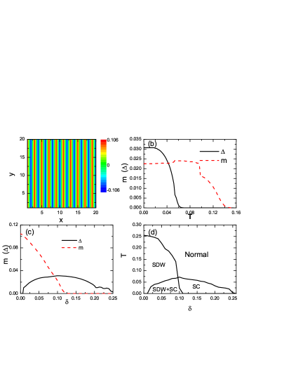
Figure 1: (Color online) (a) The intensity plot of the magnetic order at zero doping and zero temperature. (b) The magnitude of the SC order parameter $\Delta$ and magnetic order $m$ as a function of the temperature with the doping density $\delta=0.09$. (c) The magnitude of the SC order parameter $\Delta$ and magnetic order $m$ as a function of the doping at zero temperature. (d) The calculated phase diagram.

We plot the spatial distribution of the magnetic order [$m_{i}=\frac{1}{4}\sum_{\mu}(n_{i\mu\uparrow}-n_{i\mu\downarrow})$] at the zero temperature and zero doping in Fig.1(a). As seen, the magnetic spin order is antiferromagnetic along the $x$ direction and ferromagnetic along the $y$ direction, corresponding to the $(\pi,0)/(\pi,\pi)$ SDW in the extended/reduced Brillouin zone. This result is consistent with the INS experiments cruz ; che and previous theoretical calculation based on different band structure jiang . There exists another degenerate SDW state with the spin order is antiferromagnetic along $y$ direction and ferromagnetic along $x$ direction. The four-fold symmetry breaking and the presence of the SDW order are due to the Fermi surface feature nesting at low doping which will be discussed below. The magnetic order decreases as the temperature increases or doping increases. The amplitudes of the SC order and magnetic order as functions of the temperature and doping are shown in Figs.1(b) and 1(c), respectively. At the fixed doping, both the magnetic order and SC order decrease as the temperature increases and two transition temperatures are revealed, as seen in Fig.1(b). The superconductivity occurs at the doping $0.01$ and vanishes at the doping 0.26, as seen in Fig.1(c). The magnetic order is maximum at zero doping and decreases monotonically as the doping increases. The calculated phase diagram is plotted in Fig.1(d). As seen, the magnetic order and SC order coexist in the underdoped region. The magnetic order decreases abruptly and a quantum critical point $\delta=0.12$ is revealed. The superconductivity appears as the magnetic order is suppressed and the SC transition temperature T_c reaches the maximum as the magnetic order disappears. Our results are reasonably consistent with the experiments on the BaFe_2-xCo_xAs₂ pra ; les ; jul .

The real-space mean-field Hamiltonian can be transformed to the momentum space because the SC order is uniform and the magnetic order has the period $2\times 1$. The Fermi surface, defined by the zero energy contours of the quasiparticles, can be obtained through the momentum space Hamiltonian. The evolution of the normal state Fermi surface with increasing doping densities is shown in Fig.2.

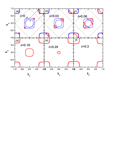
Figure 2: (Color online) The doping evolution of the Fermi surface at the temperature $T=0.1$ (i.e., the superconductivity disappears). The (red) bold solid curves and (black) dotted lines in panels (a-c) indicate the ungapped Fermi surfaces and the magnetic Brillouin zone boundary in the magnetic phase, respectively. The (blue) thin solid curves in panels (a)-(c) show the normal states Fermi surface by setting the magnetic order $m=0$.

At zero doping [Fig.2(a)], the Fermi surface in the normal state [(blue) thin lines] contains two hole pockets around point $\Gamma=(0,0)$ (labeled as $\alpha$ and $\beta$ bands) and two electron pockets around point $M=(\pi,\pi)$ (labeled as $\delta$ and $\gamma$ bands). The existence of the SDW here represents the pairing of the electron and hole. Thus in the SDW phase, the momentum of the SDW order should be consistent with the Fermi surface nesting momentum connecting the hole pockets and electron pockets. As seen in Fig.2(a), the prime nesting vector (denoted by the dashed arrows) in the reduced Brilliouin zone is $(\pi,\pi)$. As the doping increases, the hole pockets shrink. Then the nesting vector should deviate from $(\pi,\pi)$. But with the presence of the underline lattice, the nesting vector is still pinned at $(\pi,\pi)$ and this is what has been observed by experiments les , thus the magnetic order will decrease as the doping increases. When the doping increases to $\delta\thicksim 0.1$ (at $T=0.1$), there is no nesting vector that can be sustained by the lattice and the SDW order disappears. The magnetic Fermi surfaces [red (bold) solid curves] as shown in Figs.2(a-c) are represented by ungapped pockets along the $\Gamma-M$ line or $k_{x}=k_{y}$ direction. Parts of the original Fermi surface [(blue) thin solid curves] are gapped by the SDW order. The small ungapped Fermi surface pockets along the $\Gamma-M$ line is consistent with experiments on the parent compound BaAs₂Fe₂ dingh . The existence of ungapped Fermi surface pockets at zero doping [see Fig.2(a)] indicates that the parent compound is in fact not an ’insulator’ a but a poor ’metal’. Here the four-fold symmetry is broken in the magnetic phase, due to the presence of the magnetic order shown in Fig.1(a). There exists another degenerate solution with the Fermi surface pockets along the $k_{x}=-k_{y}$ direction, corresponding to the $(0,\pi)$-SDW ground state in the extended Brillouin zone. As the doping increases, the ungapped pockets become larger and larger and eventually cover the whole Fermi surface as the SDW order disappears.

As the doping increases to $\delta=0.16$, and $0.24$ [Figs.2(d) and 2(e)], the $\alpha$-band is filled by electrons completely and the Fermi surface of this band disappears, thus only three Fermi surface pockets are left. This feature is consistent with the experiments tera . As the doping density increases to about $0.30$ [Fig.2(f)], the Fermi surface pocket of $\beta$-band will also disappear and only two electron-like Fermi surface pockets are left, which is also consistent with the experiments sek . On the other hand, the electron pockets expand a little as the doping increases but relatively the electron pockets depend weakly on the doping, also in agreement with the ARPES experiments tera ; sek .

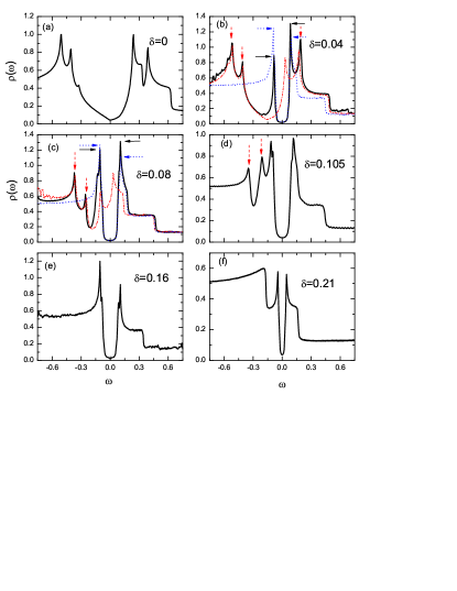
Figure 3: (Color online) The LDOS spectra with different doping densities at the zero temperature. The (red) dash-dotted and (blue) dotted lines in panels (b) and (c) are non-selfconsistent results with $\Delta\equiv 0$, and $m\equiv 0$, respectively.

We also calculate the LDOS spectra according to Eq. (9). The spectra at different doping densities are shown in Fig.3. At zero doping [Fig.3(a)], the density of states shows four well-defined coherence peaks due to the SDW order. The maximum dip of the spectrum is at the chemical potential or zero energy. Note that there are two coherence peaks at negative energies and two at positive energies. The splitting of the coherence peaks is caused by the inter-orbital coupling $t_{4}$. As the doping increases [Figs.3(b) and 3(c)], the maximum dip of the LDOS due to the $(\pi,\pi)$ SDW order is nearly independent of doping and always pinned at the chemical potential of zero doping. This is similar to the case of d-density wave in cuprate superconductors zhu . As we define the zero energy at the chemical potential, the maximum dip of the SDW spectrum will shift to the left or the negative energy as doping increases. While in the SC state, two SC coherence peaks show up, and the mid-gap point is always located at the zero energy or the chemical potential of the electron-doped system.

We now discuss the LDOS spectra in the coexisting region. In this region, the pure SC state and the pure SDW state have higher free energy. These two pure states can be obtained by setting the magnetic order $m\equiv 0$ and the SC order is calculated self-consistently and setting the SC order $\Delta\equiv 0$ and the magnetic order is obtained self-consistently, respectively. The results of the pure SC and SDW states are represented by (blue) dotted and (red) dash-dotted lines, respectively in Figs.3(b) and 3(c). In the pure SDW state, four SDW peaks are obtained with the maximum dip at the negative energy. In the pure SC state, two SC coherence peaks are seen with the mid point of the gap at the zero energy. In the coexisting state, the structure of the spectra inside the SC gap is practically the same to the spectra of the pure SC state. As shown in Figs.3(b) and 3(c), we can see clearly the previous SDW peaks outside the SC gap. But the SDW peaks inside the SC gap in the pure magnetic state cannot be seen in the coexisting state. The additional peaks outside the SC peaks, positioned by the (red) vertical arrows can be regarded as one signature of the coexistence of the magnetic and SC orders in electron-doped materials. As doping increases, only negative SDW peaks would appear, as seen in Figs.3(c) and 3(d). It is needed to point out that such structures outside the SC gap due to the SDW order as shown in Figs.3(a-d) so far have not been clearly identified by the experiments.

Another significant feature caused by the magnetic order can be seen from the intensities of the SC coherence peaks [see Figs.3(b) and 3(c)]. In pure SC state, the intensity of the SC peak at the negative energy is higher than that at the positive energy for all the doping densities we considered. These SC peaks are positioned by the parallel (blue) dotted arrows. In the coexisting region, as we mentioned above, the SDW spectra shift to the negative energy so that the SC peak at the negative energy is within the SDW gap and that at the positive energy is outside the SDW gap. Thus the intensity of the SC peak at the positive energy is enhanced and the one at the negative energy gets suppressed by the SDW order. As a result, in the coexisting state, the intensity of the SC coherence peak [denoted by the (black) solid arrows] at the negative energy is lower than that at the positive energy. The asymmetry disappears near the optimal doping $(\approx 0.105)$, as seen in Fig.3(d). In the overdoped region [see Figs.3(e) and 3(f)], the asymmetry occurs again but with the intensity of the SC peak at negative energy becoming stronger. This feature has recently been confirmed by the scanning tunneling microscopy (STM) experiments on BaFe_2-xCo_xAs₂ pan .

In summary, we have examined theoretically the coexistence of the SDW and SC orders in electron-doped iron-pnictide superconductors based on the two orbital model and BdG equations. The phase diagram is mapped out and the coexistence of the SDW and SC orders occurs at low doping. The evolution of the Fermi surface as the doping varies is presented and the results agree with several ARPES experiments. The LDOS has also been calculated from low to high doping. The signatures of the SDW order are identified and is consistent with the recent STM experiment. It is important to point out that the present results are critically dependent on the two orbital model suggested in Ref. zhang .

We thank S. H. Pan and Ang Li for useful discussion and showing us their STM data before publication. This work was supported by the Texas Center for Superconductivity at the University of Houston and by the Robert A. Welch Foundation under the Grant No. E-1146.

References

- (1) Y. Kamihara , J. Am. Chem. Soc. 130, 3296 (2008).
- (2) For a review, please see e.g., M. V. Sadovskii, Phys. Usp. 51, 1201 (2008).
- (3) J. Dong et al., Europhys. Lett. 83, 27006 (2008); V. Cvetkovic and Z. Tesanovic, Europhys. Lett. 85, 37002 (2009); R. Yu et al., Phys. Rev. B 79, 104510 (2009).
- (4) I. I. Mazin, D. J. Singh, M. D. Johannes, and M. H. Du, Phys. Rev. Lett. 101, 057003 (2008); Z. J. Yao, J. X. Li, and Z. D. Wang, New J. Phys. 11, 025009 (2009); Fa Wang, Hui Zhai, Ying Ran, Ashvin Vishwanath, and Dung-Hai Lee, Phys. Rev. Lett. 102, 047005 (2009).
- (5) J. Zhao et al., Nature Mater. 7, 953 (2008).
- (6) D. K. Pratt et al., Phys. Rev. Lett. 103, 087001 (2009); X. F. Wang et al., New J. Phys. 11, 045003 (2009); Y. Laplace, J. Bobroff, F. Rullier-Albenque, D. Colson, and A. Forget, Phys. Rev. B 80, 140501(R) (2009).
- (7) C. Lester et al., Phys. Rev. B 79, 144523 (2009); A. D. Christianson et al., Phys. Rev. Lett. 103, 087002 (2009).
- (8) M.-H. Julien et al., EuroPhys. Lett. 87, 37001 (2009).
- (9) H. Chen et al., EuroPhys. Lett. 85, 17006 (2009).
- (10) Y. Zhang et al., Phys. Rev. Lett. 102, 127003 (2009).
- (11) R. H. Liu et al., Phys. Rev. Lett. 101, 087001 (2008); A. J. Drew et al., Nature mater. 8, 310 (2009).
- (12) D. Parker, M. G. Vavilov, A. V. Chubukov, and I. I. Mazin, Phys. Rev. B 80, 100508(R) (2009); A. B. Vorontsov, M. G. Vavilov, and A. V. Chubukov, Phys. Rev. B 79, 060508(R) (2009).
- (13) D. Zhang, Phys. Rev. Lett. 103, 186402 (2009).
- (14) K. Terashima et al., Proc. Natl. Acad. Sci. U.S.A. 106, 7330 (2009).
- (15) Y. Sekiba et al., New J. Phys. 11, 025020 (2009).
- (16) K. Nakayama , Europhys. Lett. 85, 67002 (2009); H. Ding , Europhys. Lett. 83, 47001 (2008); T. Kondo , Phys. Rev. Lett. 101, 147003 (2008); D. V. Evtushinsky , Phys. Rev. B 79, 054517 (2009); C. Liu , Phys. Rev. Lett. 101, 177005 (2008); K. Hashimoto , Phys. Rev. Lett. 102, 017002 (2009).
- (17) A. V. Chubukov, D. V. Efremov, and I. Eremin, Phys. Rev. B 78, 134512 (2008).
- (18) C. de la Cruz et al., Nature (London) 453, 899 (2008).
- (19) Y. Chen et al., Phys. Rev. B 78, 064515 (2008).
- (20) A. M. Oles, G. Khaliullin, P. Horsch, and L. F. Feiner, Phys. Rev. B 72, 214431 (2005).
- (21) H. M. Jiang, J. X. Li, and Z. D. Wang, Phys. Rev. B 80, 134505 (2009).
- (22) J. X. Zhu, B. Friedman, and C. S. Ting, Phys. Rev. B 59, 3353 (1999).
- (23) W. L. Yang et al., Phys. Rev. B 80, 014508 (2009).
- (24) P. Richard et al., arxiv: 0909.0574; D. Hsieh et al., arxiv: 0812.2289; S. de Jong et al., Europhys. Lett. 89, 27007 (2010); M. Yi et al., phys. Rev. 80, 174510 (2009); S. E. Sebastian et al., J. Phys.: Condens. Matter 20, 422203 (2008); J. G. Analytis et al., Phys. Rev. B 80, 064507 (2009).
- (25) J. X. Zhu, W. Kim, C. S. Ting, and J. P. Carbotte, Phys. Rev. Lett. 87, 197001(2001); W. Kim, Jian-Xin Zhu, J. P. Carbotte, and C. S. Ting, Phys. Rev. B 65, 064502 (2002).
- (26) S. H. Pan et al., private communication.