Wavelet-based Faraday Rotation Measure Synthesis

Abstract

Faraday Rotation Measure (RM) Synthesis, as a method for analyzing multi-channel observations of polarized radio emission to investigate galactic magnetic fields structures, requires the definition of complex polarized intensity in the wavelength range $-\infty<\lambda^{2}<\infty$. The problem is that the measurements at negative $\lambda^{2}$ are not possible. We introduce a simple method for continuation of the observed complex polarized intensity $P(\lambda^{2})$ into the domain $\lambda^{2}<0$ using symmetry arguments. The method is suggested in context of magnetic field recognition in galactic disks where the magnetic field is supposed to have a maximum in the equatorial plane. The method is quite simple when applied to a single Faraday-rotating structure on the line of sight. Recognition of several structures on the same line of sight requires a more sophisticated technique. We also introduce a wavelet-based algorithm which allows us to consider a set of isolated structures in the ($\phi,\lambda^{2}$) plane (where $\phi$ is the Faraday depth). The method essentially improves the possibilities for reconstruction of complicated Faraday structures using the capabilities of modern radio telescopes.

1 Introduction

Observations of polarized radio emission are the main sources of information on magnetic fields of galaxies. The basic idea of magnetic field analysis from polarized radio emission data originates in the classical paper of Burn (1966) (for a later development see Sokoloff et al. (1998)). In particular, Burn (1966) noted that the complex polarized intensity $P$ obtained from a radio source is related to the Faraday dispersion function $F(\phi)$ as

$$P(\lambda^{2})=\int_{-\infty}^{\infty}F(\phi)e^{2i\phi\lambda^{2}}d\phi.$$ (1)

$F(\phi)$ is the fraction of radiation with the Faraday depth $\phi$ multiplied by intrinsic complex polarization and it is an important emission characteristic of interest. Here the Faraday depth $\phi$ is defined by

$$\phi(z)=-0.81\int_{z}^{0}\,B_{\parallel}n_{e}dz^{\prime},$$ (2)

where $\,B_{\parallel}$ is the line-of-sight magnetic field component measured in $\mu$G, $n_{e}$ is the thermal electron density measured in cm^-3 and the integral is taken from the observer at $z=0$ over the region which contains both, magnetic fields and free electrons, and $z$ is measured in parsecs. Following Eq. (1) $P$ is the inverse Fourier transform of $F$. Correspondingly, the Faraday dispersion function $F$ is the Fourier transform of the complex polarized intensity:

$$F(\phi)={{1}\over{\pi}}\hat{P}(k),$$ (3)

where $k=2\phi$, and the Fourier transform is defined as

$$f\left(x\right)={{1}\over{2\pi}}\int_{-\infty}^{\infty}{\hat{f}\left(k\right)e^{ikx}dk},\quad\hat{f}\left(k\right)=\int_{-\infty}^{\infty}{f\left(x\right)e^{-ikx}dx}.$$ (4)

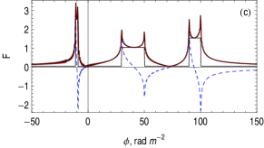
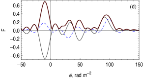
Figure 1: RM Synthesis reconstruction of a standard example from Brentjens & de Bruyn (2005): (a) initial $F(\phi)$ which is chosen purely real; (b) amplitude of $PI(\lambda^{2})$; (c) $F(\phi)$ reconstructed with whole domain $\lambda^{2}>0$: real part - thin solid, imaginary part - dashed, amplitude - thick solid; (d) $F(\phi)$ reconstructed from the data of spectral band $0.6<\lambda<0.78$ m. The spectral window of observations is indicated in panel (b) by horizontal dashed line.

Implementation of multichannel spectro-polarimetry on modern radio telescopes provided observations of $P$ over a wide range of $\lambda$ (e.g. Haverkorn et al., 2000) which made the use of Eq. (3) possible. This is the idea of Faraday Rotation Measure Synthesis (RM Synthesis) (Brentjens & de Bruyn, 2005) which opened new perspectives in investigations of magnetic field of galaxies and clusters of galaxies (Haverkorn et al., 2003; de Bruyn & Brentjens, 2005; Beck, 2009; Heald et al., 2009).

A key problem of RM Synthesis application is that $P$ is defined only for $\lambda^{2}>0$ and in practice can be observed only in a finite spectral band. Moreover, the maximum of $P$ in practice can be located outside the available spectral band (see e.g. Fig. 1b). Development of robust methods for the reconstruction of $F$ from $P$ in a given spectral range becomes crucial for the practical implementation of RM Synthesis.

Fig. 1 shows results of RM Synthesis applied to a standard test as exploited by Brentjens & de Bruyn (2005). Panel (a) shows the function $F$, which includes three real-valued box-like structures, panel (b) - the corresponding polarized intensity $P$ (the dashed horizontal line shows the spectral window $0.6<\lambda<0.78$ m). We used a channel spacing of $\delta\lambda=0.4$ cm. Hereafter, $F$ and $P$ are numerically evaluated in arbitrary but mutually consistent units. Note that $F$ is in general a complex-valued function. Its modulus defines the emission and its phase defines the intrinsic position angle. Panel (c) shows the result of the straightforward application of the RM Synthesis algorithm to the physical range $\lambda^{2}>0$, while $P(\lambda^{2})$ is set to zero for all negative $\lambda^{2}$. We see that the real part of the reconstructed signal is the same as the initial one (except that it has a twice lower amplitude), however, the reconstructed signal obtains a substantial imaginary part with a shape which is quite remote from the real part. This leads to a change of the emission distribution and a loss of any information concerning the position angle (apart from the central point of the emission region, where the position angle correctly is zero). In the context of chaotic magnetic fields in galaxy clusters this loss is less important (de Bruyn & Brentjens, 2005), but in galactic magnetic field studies it becomes crucial because the intrinsic position angle determines the orientation of the regular magnetic field component perpendicular to the line of sight. Fig. 1d shows that the reconstruction becomes much more difficult if we restrict the data to a relatively narrow spectral band $0.6<\lambda<0.78$ m. We see that even the sign of the reconstructed real part can be wrong. In that case the algorithm for finite spectral band introduced by Brentjens & de Bruyn (2005) was used.

A general message obtained from Fig. 1 is that in order to envisage possible ways to get a practical implementation of RM Synthesis one has to include some additional information based on the nature of the physical phenomena which provide the Faraday rotation. Here we concentrate our efforts on the problems associated with missing $P(\lambda^{2})$ for $\lambda^{2}<0$.

2 Improving the RM Synthesis algorithm

The complex-valued intensity of polarized radio emission for a given wavelength

$$P(\lambda^{2})=\int_{0}^{\infty}\varepsilon(z)e^{2i\chi(z)}e^{2i\phi(z)\lambda^{2}}dz,$$ (5)

is defined by the emissivity $\varepsilon$ and the intrinsic position angle $\chi$ along the line of sight. Here $z$ is the distance from observer to a point in the emitting region; the integral is taken over the whole emitting region. If the Faraday depth $\phi$ is a monotonic function of $z$ (which means that $z$ is a single-valued function of $\phi$), we can define the Faraday dispersion function as a function of Faraday depth

$$F(\phi)=\varepsilon(\phi)e^{2i\chi(\phi)}\left({d\phi}\over{dz}\right)^{-1}.$$ (6)

In the ideal case, reconstructing the Faraday dispersion function $F$ from (3) and knowing the Faraday depth $\phi$ for any $z$, one can derive the characteristics of radio emission ($\varepsilon$ and $\chi$) along the line of sight. They can be used as a tomography in order to derive some characteristics of the magnetic field distribution from $F$. The task of RM Synthesis is much more modest and concerns the reconstruction of the Faraday function from the observed polarized emission which itself is already a complicated problem.

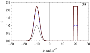
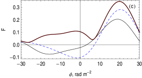
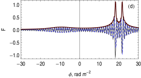
Figure 2: Standard RM Synthesis for a test Faraday dispersion function. (a) Original test function which includes one Gaussian and one box structure. Reconstructions: (b) using the whole domain $\lambda^{2}>0$, (c) using the window $0.6<\lambda<0.78$ m, (d) using the window $0.6<\lambda<2.5$ m. Real part - thin solid, imaginary part - dashed, amplitude - thick solid.

Let us consider a physically motivated simple example, i.e. $P$ produced by a two-layer system , to isolate and overcome the shortcomings of the RM Synthesis technique. Each layer contains a homogeneous magnetic field which has non-vanishing line-of-sight and perpendicular components. Both layers are thought to be emitting and rotating polarized radio waves. The corresponding $F(\phi)$ is shown in Fig. 2a. It is important for the discussion below that the analyzed signal has non-vanishing real and imaginary parts. The absolute value of $F(\phi)$ indicates how much polarized emission comes from a region with Faraday depth $\phi$ and its phase gives the intrinsic position angle (about $13^{\circ}$ and $31^{\circ}$) of the emission. Just to illustrate the variety of possible situations, we choose two different shapes of the slabs, i.e. one slab with sharp boundaries and one with a Gaussian shape.

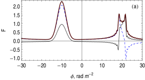
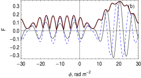
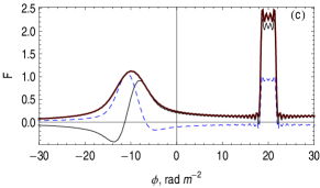
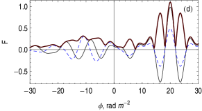
Figure 3: RM Synthesis for the test from Fig.2 using the extension of $P(\lambda^{2})$ in the domain $\lambda^{2}<0$ defined by (7). The parameter $\phi_{0}$ is adjusted to the position of the left structure (a,b) or right structure (c,d). The whole domain of $\lambda$ is used in panels (a,c) and the spectral window $0.6<\lambda<0.78$ m in panels (b,d). Real part - thin solid, imaginary part - dashed, amplitude - thick solid.

The result of the straightforward application of RM Synthesis where the integral is taken over the physically admissible region $\lambda^{2}>0$ is shown in Fig. 2b. RM Synthesis reproduces to some extent the absolute value of the signal, but fails to reproduce its phase. A naive interpretation of this result could be that field reversals occur in each layer, but is obviously incorrect. In the same figure we show the result of $F(\phi)$ reconstruction within the spectral band $0.6<\lambda<0.78$ m (panel c). Then both structures become diffuse with a more or less arbitrary phase. The last panel illustrates what happens if the upper wavelength boundary will be extended up to $\lambda=2.5$m (as expected for the Low Frequency Array (LOFAR) and the Square Kilometre Array (SKA) telescopes). This extension essentially improves the recognition of the sharp structure (the right one in the figure) but almost does not affect the reconstruction of the left (Gaussian) structure.

To avoid the non-uniqueness in the Faraday dispersion function reconstruction, some additional information (or hypothesis) is required. We suggest to improve the above reconstruction by some constraint concerning the possible symmetry of an isolated object.

Suppose that the expected objects are mainly galactic disks with magnetic fields believed to be symmetric with respect to the galactic equator. Then the desired $F$ should be even with respect to the center of the given object. Therefore, we consider each maximum of the reconstructed $F(\phi)$ separately and prescribe that the continuation of $P(\lambda^{2})$ to the region of $\lambda^{2}<0$ has to be chosen in a way which makes $F(\phi)$ symmetric with respect to the point $\phi=\phi_{0}$, where $\phi_{0}$ is the position of the maximum under consideration. This means that $F(2\phi_{0}-\phi)=F(\phi)$ and using the shift theorem one gets

$$P(-\lambda^{2})=\exp(-4i\phi_{0}\lambda^{2})P(\lambda^{2}).$$ (7)

The antisymmetric case can be considered as well with slight change in the algorithm: Eq. (7) changes to $P(-\lambda^{2})=-\exp(-4i\phi_{0}\lambda^{2})P(\lambda^{2})$.

Fig. 3 shows the results of reconstruction of the same test but following the suggested continuation. The test function includes two objects, while the algorithm includes only one parameter $\phi_{0}$. Firstly, we performed the continuation adjusting $\phi_{0}$ to the position of the left object (panel a). Then the method gives realistic result for this object. The reconstructed structure has no apparent internal field reversal and the ratio of real and imaginary parts of $F(\phi)$, i.e. the phase, is correctly reproduced. Position angles are restored with the accuracy of $3^{\circ}$. Of course, the result for the other layer, i.e. the second maximum of $|F(\phi)|$ in Fig. 3 remains false. Panel (b) shows what happens if the range of $\lambda$ covered by the observation is reduced to $0.6<\lambda<0.78$ m. Instead of one peak one gets a sequence of peaks, which is a usual result for a Fourier reconstruction using a narrow spectral window. The suggested procedure does not suppress the sidelobes in the standard Rotation Measure Spread Function (RMSF) (Heald et al., 2009) but corrects the phase within the main central peak. Of course, the amplitude of each peak is much less than the amplitude of the peak in panel (a), however, the ratio of real and imaginary parts of $F(\phi)$ in the central peak remains realistic. If the parameter $\phi_{0}$ is chosen following the position of the second object the method gives a correct reconstruction for the right layer and fails to reproduce the left one.

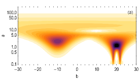
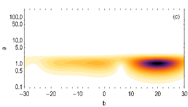
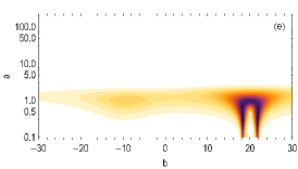
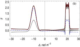
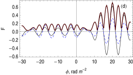
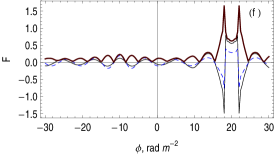
Figure 4: Wavelet-based RM Synthesis for the test from Fig.2. The modulus of wavelet coefficients on the $(a,b)$ plane (panels a,c,e) and the result of reconstruction (panels b,d,f) for whole domain of $\lambda$ (panels a,b) and the windows $0.6<\lambda<0.78$ m (panels c,d) and $0.6<\lambda<2.5$ m (panels e,f). Real part - thin solid, imaginary part - dashed, amplitude - thick solid.

An obvious shortcoming of the method exploited is its local nature: We obtain a realistic shape of a chosen maximum and ignore what happens with the other one. A natural extension is to apply the recommendation of Eq. (7) locally to each maximum. This extension brings the idea of wavelets into consideration.

3 RM Synthesis and wavelets

Wavelet transform presents a kind of “local” Fourier transform, allowing us to isolate a given structure in physical space and the Fourier space. Let us define the wavelet transform of the Faraday dispersion function $F(\phi)$ as

$$w_{F}(a,b)={{1}\over{|a|}}\int\limits_{-\infty}^{\infty}{F(\phi)\psi^{\ast}\left({\frac{\phi-b}{a}}\right)d\phi},$$ (8)

where $\psi(\phi)$ is the analyzing wavelet, $a$ defines the scale and $b$ defines the position of the wavelet. Then the coefficient $w_{F}$ gives the contribution of corresponding structure into the function $F$.

The function $F$ can be reconstructed using the inverse transform (see, e.g. Daubechies (1992))

$$F(\phi)=\frac{1}{C_{\psi}}\int\limits_{-\infty}^{\infty}{\int\limits_{-\infty}^{\infty}{\psi\left({\frac{\phi-b}{a}}\right)w_{F}\left({a,b}\right)\frac{da\,db}{a^{2}}}}.$$ (9)

The reconstruction formula (9) exists under condition that

$$C_{\psi}=\frac{1}{2}\int\limits_{-\infty}^{\infty}{\frac{|\hat{\psi}(k)|^{2}}{|k|}dk<\infty}.$$ (10)

Here $\hat{\psi}(k)=\int{\psi(\phi)e^{-ik\phi}d\phi}$ is the Fourier transform of the analyzing wavelet $\psi(\phi)$.

Let us emphasize that the inverse formula (9) is usually written for real signals. Then the scale parameter $a$ is positively defined and the integral is taken for $0<a<\infty$. In the case of a complex-valued function, the range of $a$ can be limited by positive values $a>0$ by taking a real analyzing wavelet $\psi(x)$. In general case of a complex-valued function and a complex wavelet, the scale parameter $a$ should be extended into the domain of negative values (like wave numbers in Fourier space).

For the sake of definiteness, we use as the analyzing wavelet the so-called Mexican hat $\psi(\phi)=(1-\phi^{2})\exp(-\phi^{2}/2)$. The wavelet is real, however, the function $P$ is complex, so that the wavelet coefficients $w_{F}$ are complex as well. For the chosen wavelet $w_{F}(-a,b)=w_{F}(a,b)$ and $C_{\psi}=1$.

Using the definition of the wavelet transform (8) and relation (3) we can directly define the wavelet decomposition of the Faraday dispersion function from the polarized intensity $P(\lambda^{2})$

$$w_{F}(a,b)={{1}\over{\pi}}\int\limits_{-\infty}^{\infty}{P(\lambda^{2})e^{-2ib\lambda^{2}}\hat{\psi}^{\ast}\left(-2a\lambda^{2}\right)d\lambda^{2}}.$$ (11)

Note that in the case of real $F$ the problem of negative $\lambda^{2}$ can be solved using progressive wavelets, whose Fourier image is localized in the domain of positive wave numbers. Thus using this kind of wavelets one avoids the problem of the $P(\lambda^{2})$ continuation in the domain $\lambda^{2}<0$.

For the general case, we divide Eq. (11) in two parts $w_{F}(a,b)=w_{-}(a,b)+w_{+}(a,b)$, where

$$w_{-}(a,b) = {{1}\over{\pi}}\int\limits_{-\infty}^{0}{P(\lambda^{2})e^{-2ib\lambda^{2}}\hat{\psi}^{\ast}\left(-2a\lambda^{2}\right)d\lambda^{2}},$$ (12)

$$w_{+}(a,b) = {{1}\over{\pi}}\int\limits_{0}^{\infty}{P(\lambda^{2})e^{-2ib\lambda^{2}}\hat{\psi}^{\ast}\left(-2a\lambda^{2}\right)d\lambda^{2}}.$$ (13)

We propose the following algorithm: Firstly, knowing $P(\lambda^{2})$ for $\lambda^{2}>0$ we calculate the coefficients $w_{+}(a,b)$ and we recognize the dominating structures in the map $|w_{+}(a,b)|$. The coordinate $b$ of the corresponding maximum gives us the value of $\phi_{0}^{i}$, where upper index $i$ indicates the number of the structure. Then we reconstruct the coefficients $w_{-}(a,b)$ following the idea of Eq. (7), but reformulated for the local domain in wavelet space $(a,b)$. Namely, we define

$$w_{-}(a,b)=w_{+}\left(a,2\phi_{0}^{i}(a,b)-b\right),$$ (14)

where the parameter $\phi_{0}^{i}(a,b)$ for the given point $(a,b)$ is chosen according to the structure $i$ which dominates in its vicinity.

Now we apply the suggested algorithm to the test function from Fig. 2. The map $|w_{+}(a,b)|$ presented in Fig. 4a demonstrates two well-defined structures. The $b$-coordinates of the maxima are taken as $\phi_{0}^{i}$. The result of the reconstruction (see Fig.  4b) shows that the method reproduces the amplitude and phase of $F(\phi)$ for both layers. The reconstruction here is performed using $P(\lambda^{2})$ for the whole range $\lambda^{2}>0$. The comparison of the reconstructed position angle using standard and wavelet-base RM Synthesis is shown in Fig. 5. The suggested algorithm gives correct value for $\chi$ within both emission regions. Panels (c,d) show what happens for the reconstruction using the spectral window $0.6<\lambda<0.78$ m. One can see the wavelet map is empty in its substantial part $a>2$, however, the structures remain well-recognizable (panel c). The reconstructed $F$ contains several oscillations in domains related to both layers. The amplitude of each oscillation becomes much lower than that in panel (b), however, the ratio of the real and imaginary parts in the central maxima remain correct. The third couple of panels shows the reconstruction within the extended window $0.6<\lambda<2.5$ m. This extension allows one to keep the horn-like structures in the bottom of the wavelet plane (panel e) which provide the reconstruction of sharp boundaries of the box-like structure (panel f).

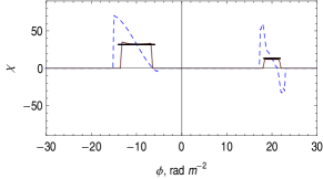
Figure 5: The intrinsic position angle $\chi$ for the test from Fig.2(a) has been reconstructed with standard (dashed) and wavelet-based (thin solid) RM Synthesis. The whole domain of $\lambda$ is used. Thick solid lines show initial $\chi$ in the location of the both structures.

4 Conclusions

The development of multi-channel observations of polarized radio emission opens promising perspectives in the understanding of cosmic magnetic fields on galactic and intergalactic scales. The first fruitful applications of RM Synthesis suggested in this context include the recognition of local structures in the Milky Way (Haverkorn et al., 2003), clusters of galaxies (de Bruyn & Brentjens, 2005) and spiral galaxies (Heald et al., 2009). However, in general the RM Synthesis algorithm contains a fundamental problem emerging from the fact that the reconstruction formula requires the definition of complex polarized intensity in the range $-\infty<\lambda^{2}<\infty$. In this paper we introduce a simple method for continuation of observed complex polarized intensity $P(\lambda^{2})$ into the domain of negative $\lambda^{2}<0$. The method is suggested in context of magnetic field recognition in galactic disks, for which the magnetic field strength is supposed to have a maximum in the equatorial plane.

The suggested method is quite simple when applied to a single structure on the line of sight. Recognition of several structures on the same line of sight requires a more sophisticated technique. The problem of structure separation is resolved using the wavelet decomposition. A simple test example demonstrates the applicability of this method. The polarization angle reconstruction is significantly improved over the standard technique. The wavelets can be useful to also overcome some other problems of RM Synthesis, related to the multi-band structure of the observational domain in $\lambda$-space, noise filtration, etc (e.g. Frick et al., 1997, 2001). The method essentially improves the possibilities for reconstruction of complicated Faraday structures using the capabilities of modern radio telescopes.

Finally note that our simple examples illustrate that the extension of the observational band into the long-wavelength domain is helpful for the recognition of structures with sharp boundaries, while the short-wavelength domain is crucial for the reconstruction of smooth structures.

References

- Beck (2009) Beck R., 2009, Rev. Mex. AyA, 36, 1
- Brentjens & de Bruyn (2005) Brentjens M. A., de Bruyn A. G., 2005, A&A, 441, 1217
- Burn (1966) Burn B. J., 1966, MNRAS, 133, 67
- Daubechies (1992) Daubechies I., 1992, Applied Mathematics, 61
- de Bruyn & Brentjens (2005) de Bruyn A. G., Brentjens M. A., 2005, A&A, 441, 931
- Frick et al. (1997) Frick P., Baliunas S. L., Galyagin D., Sokoloff D., Soon W., 1997, ApJ, 483, 426
- Frick et al. (2001) Frick P., Beck R., Berkhuijsen E. M., Patrickeyev I., 2001, MNRAS, 327, 1145
- Haverkorn et al. (2000) Haverkorn M., Katgert P., de Bruyn A. G., 2000, A&A, 356, L13
- Haverkorn et al. (2003) Haverkorn M., Katgert P., de Bruyn A. G., 2003, A&A, 403, 1031
- Heald et al. (2009) Heald G., Braun R., Edmonds R., 2009, A&A, 503, 409
- Sokoloff et al. (1998) Sokoloff D. D., Bykov A. A., Shukurov A., Berkhuijsen E. M., Beck R., Poezd A. D., 1998, MNRAS, 299, 189