Reflection of a Lieb-Liniger wave packet from the hard-wall potential

Abstract

Nonequilibrium dynamics of a Lieb-Liniger system in the presence of the hard-wall potential is studied. We demonstrate that a time-dependent wave function, which describes quantum dynamics of a Lieb-Liniger wave packet comprised of $N$ particles, can be found by solving an $N$-dimensional Fourier transform; this follows from the symmetry properties of the many-body eigenstates in the presence of the hard-wall potential. The presented formalism is employed to numerically calculate reflection of a few-body wave packet from the hard wall for various interaction strengths and incident momenta.

I Introduction

Recent intensive theoretical studies of one-dimensional (1D) Bose gases have been motivated mainly by the experimental realizations OneD ; TG2004 ; Kinoshita2006 ; Hofferberth2007 ; Amerongen2008 of the models Lieb1963 ; Girardeau1960 describing these systems. Ultracold atomic gases in tight atomic wave guides can have their transversal degrees of freedom essentially frozen such that their motion becomes effectively one-dimensional OneD ; TG2004 ; Kinoshita2006 ; Hofferberth2007 ; Amerongen2008 . These systems are described in terms of the Lieb-Liniger model, i.e., a system of identical Bose particles in 1D with pointlike $\delta$-function interactions of arbitrary strength $c$ Lieb1963 . In the limit of strong coupling $(c\rightarrow\infty)$, the Lieb-Liniger gas approaches the Tonks-Girardeau regime of impenetrable bosons Girardeau1960 , which has been experimentally achieved as well TG2004 ; the Tonks-Girardeau regime occurs at very low temperatures, low linear densities, and with strong effective interactions Olshanii ; Petrov ; Dunjko . Experiments are even capable of exploring nonequilibrium quantum dynamics of these 1D many-body systems Kinoshita2006 ; Hofferberth2007 , which may occur after some sudden change in the system’s parameters. These ultracold atomic assemblies are well isolated from the environment, that is, their quantum coherence stays preserved for long times. Therefore, they may serve as a playground to investigate relaxation of isolated quantum many-body systems, which is one of the most interesting questions in theoretical physics (e.g. see Refs. RigolNature ; Igloi2000 ; Sengupta ; Rigol2006 ; Cazallila2006 ; Calabrese2006 ; Cherng2006 ; Kollath2007 and references therein). Subsequent relaxation of 1D gases via collisions is greatly determined by the reduced dimensionality and the integrability of the underlying models. We are motivated to study the time-dependent Lieb-Liniger model because (i) today’s experiments can explore fundamental physical questions in these systems Kinoshita2006 ; Hofferberth2007 , and (ii) one can construct exact solutions of some relevant problems for all interaction strengths (from the mean field regime up to the strongly correlated regime) Gaudin1983 ; Girardeau2003 ; Buljan2008 ; Jukic2008 ; Jukic2009 ; Gritsev2009 .

The eigenstates of the Lieb-Liniger model (without an external potential present), which were constructed by employing the Bethe ansatz Lieb1963 , are determined by a set of quasimomenta; when periodic Lieb1963 boundary conditions are imposed, the quasimomenta must obey a set of transcendental Bethe equations Lieb1963 . The Lieb-Liniger eigenstates in the presence of the hard-wall (i.e., on the semi-infinite line) can be constructed via superposition of free space eigenstates Gaudin1971 ; again, if the quasimomenta should obey a particular set of transcendental equations Gaudin1971 , this superposition yields eigenstates in an infinitely deep box Gaudin1971 . Recent years have witnessed an increasing interest in exact solutions of these models (e.g., see Busch1998 ; Muga1998 ; Sakmann2005 ; Batchelor2005 ; Kinezi2006 ; Sykes2007 ; Kanamoto2009 and references therein), most of which are focused on the properties of the ground and excited eigenstates (see also Refs. Korepin1993 ; Gaudin1971a ). Unfortunately, the Lieb-Liniger model does not reveal exact solutions in the presence of some external trapping potential $V(x)$ (e.g., the harmonic potential).

In the Tonks-Girardeau limit $c\rightarrow\infty$, the methods for finding eigenstates Girardeau1960 , time-dependent solutions Girardeau2000 , as well as observables (e.g., see Ref. Rigol2005 for the system of hard-core bosons on the lattice and Pezer2007 for the continuous Tonks-Girardeau model) are much simpler due to the Fermi-Bose mapping, which in a simple fashion maps a fermionic wave function describing spinless noninteracting fermions onto a Tonks-Girardeau wave function Girardeau1960 ; Girardeau2000 . It is important to emphasize that these methods are valid for any external potential. Perhaps the simplicity of the methods and phenomenological relevance of the model Kinoshita2006 have lead to increasing interest in quantum many-body dynamics of Tonks-Girardeau gases. Some of these studies include dynamics during free expansion Rigol2005 ; Minguzzi2005 ; DelCampo2006 ; Gangardt2008 , dynamics of dark soliton-like states Girardeau2000 , and reflections from a periodic potential Pezer2007 .

In the case of finite interaction strength $c$, it is far more difficult to calculate exact many-body wave functions and/or observables describing dynamics of time-dependent Lieb-Liniger wave packets. Without attempting to provide a review, let us mention a few approaches utilized to study nonequlibrium dynamics of 1D interacting Bose gases. The hydrodynamic formalism Dunjko (the local density approximation) can be formulated in terms of the Nonlinear Schrödinger like equation with variable nonlinearity Ohberg2002 ; this approach reduces to the Gross-Pitaevskii theory in the weakly interacting limit Dunjko ; Ohberg2002 . More sophisticated numerical approaches include the time-evolving block decimation algorithm Vidal2004 , which has recently been utilized to study relaxation following a quench in a 1D Bose gas Muth2009 , the two particle irreducible (2PI) effective action approach AMRey2004 ; Gasenzer2005 , the multiconfigurational time-dependent Hartree method for bosons (MCTDHB) Alon2008 (the MCTDHB method is numerically exact when sufficiently many time-dependent orbitals are taken into account), and the multiconfigurational time-dependent Hartree method (e.g., see Ref. Zollner2008 and references therein). Reference Gritsev2009 provides a discussion of several methods which can be used to describe nonequilibrium dynamics of Lieb-Liniger gases with greater focus on the form-factor approach Gritsev2009 , which has been recently utilized to calculate equilibrium correlation functions of a 1D Bose gas (see Caux2007 and references therein). A broader review discussing many-body physics with ultracold gases can be found in Ref. Bloch2008 . We also mention a recent review on quantum transients delCampo2009 .

An interesting exact method has been outlined by Gaudin way back in 1983 Gaudin1983 : A time-dependent Lieb-Liniger wave function on an infinite line, in the absence of an external potential, can be constructed by acting with a differential operator (which contains the interaction strength parameter $c$) onto a time-dependent wave function describing noninteracting (spin polarized) 1D fermions Gaudin1983 ; Buljan2008 ; Jukic2008 ; Jukic2009 ; Pezer2009 . For dynamics of a Lieb-Liniger wave packet comprised of $N$ particles, this method reduces to finding an $N$-dimensional Fourier transform, which can be used to extract the asymptotic behavior of the wave function and some observables during the course of 1D free expansion Jukic2008 ; Jukic2009 . In this article we investigate the possibility of extending this approach to study dynamics of a Lieb-Liniger wave packet in the presence of the hard-wall potential.

Our interest in quantum dynamics in the presence of the hard-wall potential is in part motivated by experiments. More specifically, the interaction of Bose-Einstein condensates (BEC) with surfaces is of interest for implementations of atom interferometry on chips Wang2005 . A BEC falling under gravity, and then reflecting from a light-sheet, has been experimentally and theoretically studied in Ref. Bongs1999 . Moreover, one of the prominent experimental activities nowadays is deceleration of atomic beams by reflection from a moving mirror. This work first started with neutrons being cooled by reflecting from a moving Ni surface neutron . In cold atoms physics, there have been several experiments for manipulation and slowing down atomic beams with the use of reflection mirrors Libson2006 ; Narevicius2007 ; Reinaudi2006 .

Here we explore, by using exact methods, dynamics of Lieb-Liniger wave packets in the presence of the hard-wall potential, more specifically, reflection of a Lieb-Liniger wave packet from such a wall. The outline of the paper is as follows. In Sec. II we introduce the model and outline the construction of eigenstates in the given external potential. In Sec. III we analytically discuss time-dependent quantum dynamics of the system which starts from a general initial condition. By employing the symmetries of the Lieb-Liniger eigenstates, we demonstrate that a time-dependent Lieb-Liniger wave packet reflecting from the wall can be calculated by solving an $N$-dimensional Fourier transform, where $N$ is the number of particles. This opens the way to calculate the asymptotic properties of the wave packet by employing the stationary phase approximation as in Refs. Jukic2008 ; Jukic2009 for free expansion. In Sec. IV we utilize the formalism to numerically study dynamics of single-particle density and momentum distribution of a few-body wave packet reflecting from the wall. We find that the wave packets for smaller interaction strength $c$ get reflected at a slower rate, because they get compressed more strongly as the wave packet hits the wall. The interference fringes which occur during the dynamics have larger visibility for smaller values of $c$.

II Eigenstates in the presence of the hard-wall potential

The Lieb-Liniger model describes $N$ identical bosons in one spatial dimension, which interact via a repulsive $\delta$-function potential of strength $c>0$. The model can be represented in terms of the Schrödinger equation:

$$i\frac{\partial\psi}{\partial t}=-\sum_{i=1}^{N}\frac{\partial^{2}\psi}{\partial x_{i}^{2}}+\sum_{1\leq i<j\leq N}2c\,\delta(x_{i}-x_{j})\psi+\sum_{i=1}^{N}V(x_{i})\psi(x_{1},\ldots,x_{N},t).$$ (1)

As we have already stated, this model can be experimentally realized with ultracold atoms in tight atomic waveguides. The spatial and temporal coordinates ($x$ and $t$, respectively), as well as the potential $V(x)$ are dimensionless in this paper. Their connection to physical units is as follows: $x=X/X_{0}$, $t=T/T_{0}$, and $V(x)=U(X)/E_{0}$, where $X$, $T$ and $U(X)$ are space, time, and energy variables in physical units. Given the mass of the atoms $m$, the choice of an arbitrary length scale $X_{0}$ sets the time scale $T_{0}=2mX_{0}^{2}/\hbar$, and energy scale $E_{0}=\hbar^{2}/(2mX_{0}^{2})$. Suppose that the transverse confinement of the atomic waveguide is described by a harmonic oscillator with frequency $\omega_{\perp}$. The interaction parameter $c$ is proportional to the effective 1D coupling strength $g_{1D}$ Olshanii , $2c=g_{1D}/(X_{0}E_{0})=g_{1D}\ 2mX_{0}/\hbar^{2}$, which is related to the 1D scattering length $a_{1D}$ via $g_{1D}=-2\hbar^{2}/ma_{1D}$; the 1D scattering length $a_{1D}=-(l_{\perp}^{2}/a)(1-Ca/\sqrt{2}l_{\perp})$ depends on three-dimensional scattering length $a$ and the transverse oscillator width $l_{\perp}=\sqrt{\hbar/m\omega_{\perp}}$ (the constant $C=1.4603\ldots$).

In the present paper, we focus ourselves on the dynamics (in time) of a Lieb-Liniger wave packet in the presence of the hard-wall potential, that is,

$$V(x)=\begin{cases}0,&\mbox{if }x>0\\ \infty,&\mbox{if }x\leq 0.\end{cases}$$ (2)

We will show that the solution of this problem can be constructed by solving an $N$-dimensional Fourier transform. To this end, we need eigenstates of a Lieb-Liniger gas in the hard-wall potential. First, let us write down the Lieb-Liniger eigenstates in free space (i.e., $x\in(-\infty,\infty)$ without external potentials and any boundary conditions):

$$\psi_{\{k\}} = \mathcal{N}(\{k\})\sum_{P}(-1)^{P}\prod_{i<j}{\left[\mbox{sgn}(x_{j}-x_{i})+\frac{i}{c}(k_{Pj}-k_{Pi})\right]}e^{i\sum_{j}k_{Pj}x_{j}}$$ (3)

$$= \mathcal{N}(\{k\})\sum_{P}(-1)^{P}a(P,\{k\})e^{i\sum_{j}k_{Pj}x_{j}}$$

where $\{k\}=\{k_{m}\,|\,m=1,\ldots,N\}$ is a set of (real) distinct quasimomenta which uniquely determine the eigenstate, $P$ denotes a permutation of $N$ numbers, $P\in S_{N}$, and we have implicitly defined $a(P,\{k\})$. The normalization of these eigenstates is given by Korepin1993 ; Gaudin1971a

$$\frac{1}{\mathcal{N}({\{k\}})}=\sqrt{N!(2\pi)^{N}\prod_{i<j}{\left[1+\left(\frac{k_{j}-k_{i}}{c}\right)^{2}\right]}},$$

that is, within the fundamental sector in $k$-space, $k_{1}<\cdots<k_{N}$ and $k^{\prime}_{1}<\cdots<k^{\prime}_{N}$, we have

$$\int_{-\infty}^{\infty}\psi_{\{k\}}^{*}\psi_{\{k^{\prime}\}}dx_{1}\cdots dx_{N}=\prod_{j=1}^{N}{\delta(k_{j}-k^{\prime}_{j})}.$$ (4)

The Lieb-Liniger eigenstates in the presence of the hard-wall (denoted by $\phi_{\{k\}}$) were first constructed by Gaudin Gaudin1971 as a superposition of $2^{N}$ free-space eigenstates. This superposition obeys the hard-wall boundary condition: $\phi_{\{k\}}(x_{1}=0,x_{2},\ldots,x_{N})=0$ in the fundamental sector $R_{1}:x_{1}<x_{2}<\ldots<x_{N}$ of $x$-space. These eigenstates are expressed as follows:

$$\phi_{\{k\}}=\sum_{\{\epsilon\}}A(\{\epsilon\},\{k\})\psi_{\{\epsilon k\}},$$ (5)

where $\{\epsilon\}=\{\epsilon_{m}\,|\,\epsilon_{m}\in\{-1,1\},m=1,\ldots,N\}$ and $\{\epsilon k\}=\{\epsilon_{m}k_{m}\,|\,\epsilon_{m}\in\{-1,1\},m=1,\ldots,N\}$; evidently, there are $2^{N}$ such sets and therefore $2^{N}$ terms in the sum (5). The quantity $A(\{\epsilon\},\{k\})$ is defined by

$$A(\{\epsilon\},\{k\})=\epsilon_{1}\cdots\epsilon_{N}\ A^{\prime}(\epsilon_{1}k_{1},\epsilon_{2}k_{2},\ldots,\epsilon_{N}k_{N}),$$ (6)

where

$$A^{\prime}(k_{1},k_{2},\ldots,k_{N})\equiv\frac{\prod_{i<j}{\left[1+\frac{i}{c}(k_{j}+k_{i})\right]}}{\sqrt{\prod_{i<j}{\left[1+\left(\frac{k_{j}+k_{i}}{c}\right)^{2}\right]}}},$$ (7)

are the coefficients utilized in the superposition. It is straightforward to verify that indeed $\phi_{\{k\}}(x_{1}=0,x_{2},\ldots,x_{N})=0$ in the fundamental sector $R_{1}$ Gaudin1971 .

However, it is not simple to prove that these eigenstates are orthogonal and normalized. This is of key importance if one wishes to project some initial state onto these eigenstates and calculate time-evolution in the standard fashion via superposition over eigenstates. In Section IV we discuss the normalization of eigenstates (5), and based on our numerical investigations conjecture that these eigenstates are orthogonal and normalized.

III Many-body dynamics in time via a Fourier transform

In this section we demonstrate that a solution of the time-dependent equation (1) with the hard-wall potential (2) can be expressed in terms of an $N$-dimensional Fourier transform. We assume that at time $t=0$ the wave packet is localized in the vicinity of the wall. For example, the initial state $\psi_{0}$ can be the ground state wave function in some external trapping potential; if at $t=0$ this potential is suddenly turned off, the wave packet will start expanding and some of its components will be reflected from the wall which will give rise to interference effects. Such a scenario is possible to create with today’s experimental capabilities Kinoshita2006 . One possible (similar) scenario is as follows: suppose that at $t=0$ the aforementioned trapping potential is turned off, and that in the next instance the many body wave packet is given some momentum kick, say towards the wall; the reflection and interference phenomena will depend on the interactions and imparted momentum. During the reflection, particles will collide and one may ask to which extent will the initial conditions be forgotten (or blurred) after the reflection?

To describe quantum dynamics from the initial conditions described above, we write the initial state $\psi_{0}$ as a superposition over complete set of eigenstates $\phi_{\{k\}}$:

$$\psi_{0}=\int_{0<k_{1}<\cdots<k_{N}}b(k_{1},\ldots,k_{N})\phi_{\{k\}}dk_{1}\ldots dk_{N}.$$ (8)

The subsequent derivation is based on the following two relations obeyed by the eigenstates $\phi_{\{k\}}$:

$$\phi_{\{k\}}=(-1)^{P}\phi_{\{Pk\}},$$ (9)

and

$$\phi_{\{k\}}=-\phi_{\{k_{1},\ldots,k_{j-1},-k_{j},k_{j+1}\ldots,k_{N}\}}.$$ (10)

Equation (9) follows from the definition of $\phi_{\{k\}}$ in Eq. (5), and the fact that the Lieb-Liniger eigenstates in free space $\psi_{\{k\}}$ obey identical relation: $\psi_{\{k\}}=(-1)^{P}\psi_{\{Pk\}}$; this identity can be traced to the fact that $\psi_{\{k\}}$ are antisymmetric with respect to the interchange of any two variables $k_{i}$ and $k_{j}$ Korepin1993 . The derivation of Eq. (10) is straightforward. Let us define a set $\{\epsilon^{\prime}\}$, which corresponds to the set $\{\epsilon\}$ as follows: $\{\epsilon^{\prime}_{1},\ldots,\epsilon^{\prime}_{N}\}=\{\epsilon_{1},\ldots,\epsilon_{j-1},-\epsilon_{j},\epsilon_{j+1},\ldots,\epsilon_{N}\}$; it is evident from the definition (5) that $\phi_{\{k\}}=\sum_{\{\epsilon^{\prime}\}}A(\{\epsilon^{\prime}\},\{k\})\psi_{\{\epsilon^{\prime}k\}}$. Furthermore, let us denote $\{k^{\prime}\}=\{k_{1},\ldots,k_{j-1},-k_{j},k_{j+1}\ldots,k_{N}\}$, i.e., the set of $k$-values $\{k^{\prime}\}$ is identical to the set $\{k\}$ except that $k_{j}$ is reversed in sign. By using $A(\{\epsilon\},\{k\})=-A(\{\epsilon^{\prime}\},\{k^{\prime}\})$ and $\{\epsilon^{\prime}k^{\prime}\}=\{\epsilon k\}$ we have

$$\phi_{\{k^{\prime}\}}=\sum_{\{\epsilon^{\prime}\}}A(\{\epsilon^{\prime}\},\{k^{\prime}\})\psi_{\{\epsilon^{\prime}k^{\prime}\}}=-\sum_{\{\epsilon\}}A(\{\epsilon\},\{k\})\psi_{\{\epsilon k\}}=-\phi_{\{k\}},$$ (11)

that is, we obtain Eq. (10). We note in passing that if any $k_{j}=0$, then $\phi_{\{k\}}=0$, which follows from Eq. (10); furthermore, $\phi_{\{k\}}$ is also zero whenever any two of the quasimomenta $k_{i}$ and $k_{j}$ are equal.

Due to the symmetry of the hard-wall eigenstates $\phi_{\{k\}}$ presented in Eqs. (9) and (10), a complete set of eigenstates is spanned in the region of the $k$-space defined by $0<k_{1}<\ldots<k_{N}$, which we will refer to as the fundamental region in $k$-space, and denote it with $Q_{1}^{+}$. Hence, the integral in Eq. (8) spans over $Q_{1}^{+}$. Furthermore, by employing relations (9) and (10), $\psi_{0}$ can be written as an integral over the whole $k$-space:

$$\psi_{0}=\int_{-\infty}^{\infty}dk_{1}\cdots dk_{N}G(k_{1},\ldots,k_{N})e^{i\sum_{j}k_{j}x_{j}},$$ (12)

where the function $G$ is defined as

$$G(k_{1},\ldots,k_{N})=b(k_{1},\ldots,k_{N})A^{\prime}(k_{1},\ldots,k_{N})\mathcal{N}(\{k\})\prod_{i<j}{\left[\mbox{sgn}(x_{j}-x_{i})+\frac{i}{c}(k_{j}-k_{i})\right]}.$$ (13)

From Eq. (13) it immediately follows that the time-evolution of a Lieb-Liniger wave packet in the presence of the hard-wall can be calculated from an $N$-dimensional Fourier transform.

In order to derive Eqs. (12) and (13), first note that due to (9) and (10), the projection coefficients satisfy

$$b(k_{1},\ldots,k_{N})=(-1)^{P}b(k_{P1},\ldots,k_{PN}),$$ (14)

and

$$b(k_{1},\ldots,k_{N})=-b(k_{1},\ldots,k_{j-1},-k_{j},k_{j+1},\ldots,k_{N});$$ (15)

the latter identity can conveniently be rewritten as

$$b(k_{1},\ldots,k_{N})=\epsilon_{1}\cdots\epsilon_{N}b(\epsilon_{1}k_{1},\ldots,\epsilon_{N}k_{N}).$$ (16)

By employing the symmetries of the Lieb-Liniger hard-wall eigenstates, which are inherited by the expansion coefficients $b(k_{1},\ldots,k_{N})$, Eq. (8) can be rewritten as follows:

$$\psi_{0} =\frac{1}{N!}\int_{k_{1}>0,\ldots,k_{N}>0}dk_{1}\cdots dk_{N}b(k_{1},\ldots,k_{N})\ \sum_{\{\epsilon\}}A(\{\epsilon\},\{k\})$$

$$\times\mathcal{N}(\epsilon_{1}k_{1},\ldots,\epsilon_{N}k_{N})\sum_{P}{(-1)^{P}a(P,\{\epsilon k\})e^{i\sum_{j}\epsilon_{Pj}k_{Pj}x_{j}}}$$ (17)

$$=\frac{1}{N!}\int_{k_{1}>0,\ldots,k_{N}>0}dk_{1}\cdots dk_{N}\ \sum_{\{\epsilon\}}b(\epsilon_{1}k_{1},\ldots,\epsilon_{N}k_{N})A^{\prime}(\epsilon_{1}k_{1},\ldots,\epsilon_{N}k_{N})$$

$$\times\mathcal{N}(\epsilon_{1}k_{1},\ldots,\epsilon_{N}k_{N})\sum_{P}{(-1)^{P}a(P,\{\epsilon k\})e^{i\sum_{j}\epsilon_{Pj}k_{Pj}x_{j}}}$$ (18)

$$=\frac{1}{N!}\int_{-\infty}^{\infty}dk_{1}\cdots dk_{N}\ b(k_{1},\ldots,k_{N})A^{\prime}(k_{1},\ldots,k_{N})$$

$$\times\mathcal{N}(k_{1},\ldots,k_{N})\sum_{P}{(-1)^{P}a(P,\{k\})e^{i\sum_{j}k_{Pj}x_{j}}}$$ (19)

$$=\frac{1}{N!}\sum_{P}\int_{-\infty}^{\infty}dk_{1}\cdots dk_{N}\ b(k_{P1},\ldots,k_{PN})A^{\prime}(k_{P1},\ldots,k_{PN})$$

$$\times\mathcal{N}(k_{P1},\ldots,k_{PN})a(P,\{k\})e^{i\sum_{j}k_{Pj}x_{j}}$$ (20)

$$=\frac{1}{N!}\sum_{P}\int_{-\infty}^{\infty}dk_{P1}\cdots dk_{PN}\ b(k_{P1},\ldots,k_{PN})A^{\prime}(k_{P1},\ldots,k_{PN})$$

$$\times\mathcal{N}(k_{P1},\ldots,k_{PN})a(P,\{k\})e^{i\sum_{j}k_{Pj}x_{j}},$$ (21)

from which we immediately obtain Eqs. (12) and (13) because the sum over all permutations $P$ is a sum over $N!$ identical integrals. In the derivation above, the first identity, Eq. (17), follows from the properties (9) and (14). The second identity (18) is due to (16) and the definition of $A(\{\epsilon\},\{k\})$ in Eq. (6). By employing Eqs. (10) and (16), the sum over $\{\epsilon\}$ in Eq. (18) can be replaced by integrating over the whole $k$-space to obtain the third equality, Eq. (19). By using identities $A^{\prime}(k_{P1},\ldots,k_{PN})=A^{\prime}(k_{1},\ldots,k_{N})$ and $\mathcal{N}(k_{P1},\ldots,k_{PN})=\mathcal{N}(k_{1},\ldots,k_{N})$, together with Eq. (14), we obtain (20).

The time-dependent solution of the many-body Schrödinger Eq. (1) with $V(x)$ given by (2) is simply

$$\psi=\int_{-\infty}^{\infty}dk_{1}\ldots dk_{N}G(k_{1},\ldots,k_{N})e^{i\sum_{j}(k_{j}x_{j}-k_{j}^{2}t)}.$$ (22)

Thus, by knowing the function $G$ which contains all information about the initial condition, and which is simply related to the projection coefficients $b(k_{1},\ldots,k_{N})$ of the initial state onto hard-wall Lieb-Liniger eigenstates $\phi_{\{k\}}$, we can compute the time-dependent Lieb-Liniger wave function in the hard-wall potential by employing the Fourier transform. With this identification, an exact analysis of this many-body problem is at least conceptually considerably simplified.

We note that the asymptotic behavior of the many-body state and the observables such as single-particle density or momentum distribution can be straightforwardly extracted from expression (22) by using the stationary phase approximation, as it was done in Refs. Jukic2008 ; Jukic2009 for the case of free expansion of a Lieb-Liniger gas [e.g., see Eq. (15) in Ref. Jukic2008 , and Eqs. (18) and (19) in Ref. Jukic2009 ]. From these methods, and Eqs. (22) and (13), it follows that the initial conditions are imprinted into asymptotic states. It is straightforward to infer that the asymptotic wave functions, $\psi_{\infty}(\eta_{1},\ldots,\eta_{N},t)=\psi(\eta_{1}t,\ldots,\eta_{N}t,t)$ for sufficiently large $t$, vanish at the hyperplanes of contact between particles $\eta_{i}=\eta_{j}$ ($i\neq j$), which is characteristic for Tonks-Girardeau wave functions Girardeau1960 . However, it should be emphasized that the properties of such asymptotic states can considerably differ from the physical properties of a Tonks-Girardeau gas in the ground state of some trapping potential Jukic2008 (see also the second item of Ref. Buljan2008 ). Moreover, the asymptotic momentum distribution coincides, up to a simple scaling transformation, with the shape of the asymptotic single-particle density in $x$-space, reflecting the fact that the dynamics is asymptotically ballistic Jukic2009 ; this means that at asymptotic times, despite of the fact that the wave functions have attained the Tonks-Girardeau structure, interactions do not affect the dynamics any more. From the connection between the asymptotic momentum distribution and single-particle density one finds that the asymptotic momentum distribution is zero at $k=0$, and it is located on the positive $k$-axis, which simply means that for sufficiently large times the particles move away from the wall.

IV Example: A Lieb-Liniger wave packet incident on the hard wall

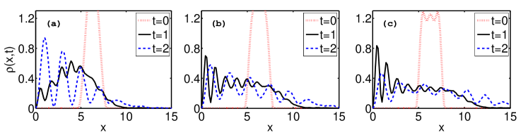
Figure 1: (color online) Density evolution of a Lieb-Liniger wave packet comprised of $N=3$ bosons, which is given some momentum kick $K$ (per particle) towards the wall. Insets correspond to the interaction strengths (a) $c=0.25$, (b) $c=3$, and (c) $c=10$. The imparted momentum is $K=1$. Red dotted lines are for $t=0$, black solid lines are for $t=1$, and blue dashed-lines are for $t=2$.

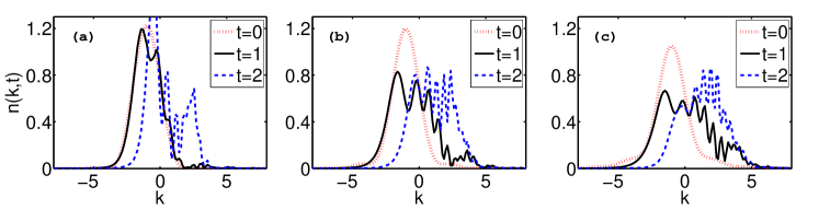
Figure 2: (color online) The same as in Fig. 1 but for the momentum distribution

In this section we study a specific example of a localized Lieb-Liniger wave packet comprised of a $N=3$ particles reflecting from the hard-wall potential. More specifically, we assume that for $t<0$ the Lieb-Liniger system is in the ground state of an infinitely deep box denoted by $\psi_{g.s.}(x_{1},x_{2},x_{3})$. The analytic expression for this ground state was found in Ref. Gaudin1971 ; for reasons of completeness, in Appendix A we present its construction. In our simulations, the box is in the interval $[1.5\pi,2.5\pi]$, i.e., $\psi_{g.s.}(x_{1},x_{2},x_{3})$ is zero whenever any $x_{i}$ is outside of this interval. At $t=0$ the box potential is suddenly turned off, and the wave packet is simultaneously (and suddenly) imparted some momentum of magnitude $K\geq 0$ towards the wall: $\psi(x_{1},x_{2},x_{3},t=0)=\psi_{g.s.}(x_{1},x_{2},x_{3})\exp[-iK(x_{1}+x_{2}+x_{3})]$; apparently, $K$ denotes the imparted momentum per particle. From such an initial state, we are able to find projection coefficients $b(k_{1},k_{2},k_{3})$ defined in Eq. (8), that is, we can find the corresponding function $G(k_{1},k_{2},k_{3})$ which is needed to calculate the Fourier transform (22). The Fourier integral in (22) is in this particular example $3$-dimensional, and it is calculated numerically by using the fast Fourier transform algorithm in MATLAB. This provides us with the time-dependent wave function $\psi(x_{1},x_{2},x_{3},t)$, which we use to study dynamics of observables such as the single-particle (SP) density $\rho(x,t)$ or the momentum distribution $n(k,t)$.

First, let us explore the effect of the interactions on the reflections of a few-body Lieb-Liniger wave packet. In Figures 1 and 2 we plot the time-evolution of single-particle densities and distributions of the momenta, respectively. The plots are made at three different times, $t=0$, $1$, and $2$, and for three values of the coupling parameter, $c=0.25$, $3$, and $10$. The magnitude of the imparted momentum per particle is $K=1$. Note that the wave packets broaden in time due to the repulsive interactions between the particles, and also due to the wave dispersion effects; the wave packets for larger values of $c$ spread at a faster rate than the wave packets for smaller $c$. From Figs. 1 and 2 we observe that wave packets with a larger interaction parameter $c$ get reflected faster than the wave packets for smaller $c$; for wave packets with smaller repulsion between the particles (smaller $c$), the compression of the wave packet is stronger, and therefore reflection of the momenta occurs at a slower rate. We also observe that all wave packets exhibit interference fringes during the reflection process. However, we find the interference fringes to be deeper for smaller values of $c$, which follows from the fact that the wave packets for smaller $c$ are more spatially coherent. This can be seen also from Fig. 2 which displays momentum distributions. The distribution $n(k,t)$ for $c=0.25$, at the largest time shown $t=2$, has one strong well-defined peak (the one closest to zero), and several smaller peaks of the wave components with larger magnitude of the momentum [see Fig. 2(a)]. In contrast, for $c=10$ this most dominant peak close to $k=0$ is much smaller [see Fig. 2(c)].

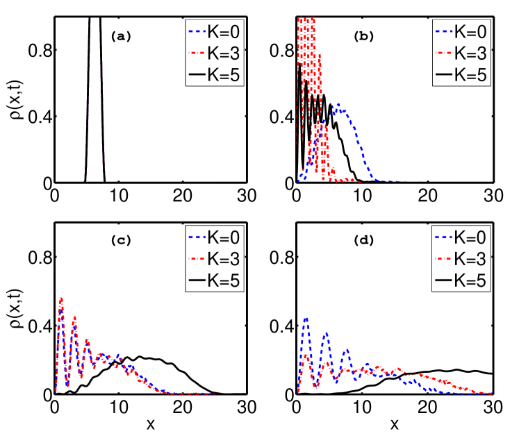
Figure 3: (color online) Density evolution of a Lieb-Liniger wave packet comprised of $N=3$ bosons, which is given some momentum kick $K$ (per particle) towards the wall. Insets correspond to the times (a) $t=0$, (b) $t=1$, (c) $t=2$, and (d) $t=3$. The interaction strength is $c=1$. Blue dashed-lines are for $K=0$, red dot-dashed lines are for $K=3$, and black solid lines are for $K=5$.

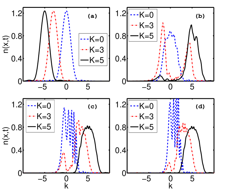
Figure 4: (color online) The same as in Fig. 3 but for the momentum distribution

Next we explore dependence of the time-evolution on the imparted momentum. To this end we fix the interaction strength at $c=1$, and observe the time-evolution for three different initial conditions (see Figs. 3 and 4): (i) expansion in the presence of the wall occurs when $K=0$, (ii) reflection at an intermediate value $K=3$, and (iii) for large value of the imparted momentum $K=5$. The wave packets for $K=3$ and $5$ have the property that basically all of the initial momentum distribution is directed towards the wall, i.e., the distributions at $t=0$ is on the negative $k$-axis. In contrast, exactly half of the initial momentum distribution of the wave packet for $K=0$ is positive (negative). The basic distinction between these cases is that the wave packets with sufficiently large imparted momentum $K$ get simply reflected from the wall and at larger times the interference fringes are almost negligible. For example, the wave packet with $K=5$ is practically completely reflected from the wall at $t=2$, see solid black lines in Figs. 3(c) and 4(c); the momentum distribution is on the positive $k$-axis and the interference fringes are essentially absent. In contrast, for $K=0$ half of the momentum distribution is already positive (corresponding to motion away from the wall), and this part interferes with the reflected component at all times of the evolution. Note that the wave packet with $K=0$ is still in the process of reflection from the wall at $t=2$ because a large fraction of its momentum distribution is still on the negative $k$-axis, see dashed blue line in Fig. 4(c); the interference fringes are the largest in this case, see dashed blue line in Fig. 3(c).

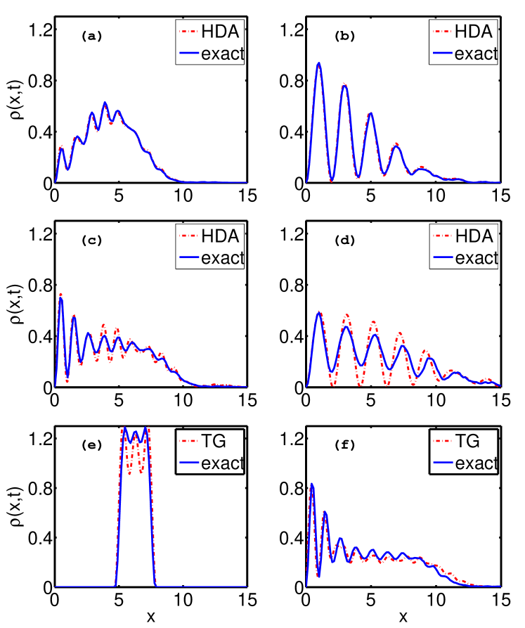
Figure 5: (color online) Comparison of the density evolution in the exact calculation, with the hydrodynamic approximation (HDA) [(a)-(d)], and the Fermi-Bose mapping [(e) and (f)] valid in the Tonks-Girardeau (TG) regime. The interaction strengths $c$ and times $t$ in the insets are: (a) $c=0.25$, $t=1$; (b) $c=0.25$, $t=2$; (c) $c=3$, $t=1$; (d) $c=3$, $t=2$; (c) $c=10$, $t=0$; (d) $c=10$, $t=1$. The initially imparted momentum is $K=1$ for all figures.

Exact solutions can serve as a benchmark to check the range of validity of other methods which may be used to analyze nonequilibrium dynamics of interacting systems. We have compared the solutions obtained with the Fourier transform method presented here with the so-called hydrodynamic formalism Dunjko , which describes the Lieb-Liniger system via the nonlinear Schrödinger equation with variable nonlinearity Ohberg2002 . In Figs. 5 (a)-(d), we show density profiles for two different couplings ($c=0.25$ and $c=3$) at two different times ($t=1$ and $t=2$). We find that the single-particle density (and momentum distribution), calculated within this method, are in good agreement with our simulations for small values of the coupling parameter $c$ (up to $c=1$); this upper limit for $c$ also depends on the initial density of the 1D Bose gas, as it is well known that the effective interaction strength parameter is $c$ divided by the linear density Lieb1963 . However, for larger values of $c$, the hydrodynamic formalism goes beyond its range of validity for the simulations presented here. For example, for the simulations at intermediate interaction strength $c=3$ [see Figs. 5 (c) and (d)], the hydrodynamic formalism predicts deeper interference fringes than those obtained via the Fourier transform method; this is attributed to the fact that the hydrodynamic formalism overestimates the spatial coherence of the wave packet Dunjko ; Ohberg2002 . For sufficiently large $c$, the system is in the Tonks-Girardeau regime, and one can employ the Fermi-Bose mapping Girardeau1960 ; Girardeau2000 to study the dynamics. In Fig. 5 (e) and (f) we compare our calculation with that obtained via Fermi-Bose mapping ($c=\infty$, Girardeau1960 ; Girardeau2000 ) for a large value of the interaction strength $c=10$; we observe that qualitative features of the Tonks-Girardeau regime such as the $N$ peaks in the initial single-particle density coincide in the two calculations, however, even larger $c$ is needed to obtain better quantitative agreement.

IV.1 Normalization of eigenstates

In order to numerically check our conjecture that the Lieb-Liniger hard-wall eigenstates defined in (5) are properly normalized, we have compared the initial state obtained via $\psi_{g.s.}(x_{1},x_{2},x_{3})\exp[-iK(x_{1}+x_{2}+x_{3})]$, and the wave function obtained via Eq. (12) by employing the function $G(k_{1},k_{2},k_{3})$, which is calculated from the projection coefficients $b(k_{1},k_{2},k_{3})$ as in Eq. (13). We found that the relative agreement between the two wave functions is on the order of $1$% or better, which is on the order of the numerical accuracy for the size of our numerical grid, which is limited by computer memory. We have performed this comparison for various initial conditions (different $K$ and $c$ values). Unfortunately, a rigorous proof of normalization of Lieb-Liniger hard-wall eigenstates is to the best of our knowledge still lacking.

IV.2 Connection to physical units

If we consider a system of ⁸⁷Rb atoms, then the ratio $X_{0}^{2}/T_{0}\approx 3.65\times 10^{-10}$m²/s is fixed. By choosing for example $X_{0}\approx 1.35\,\mu$m for the spatial scale, the temporal scale is set to $T_{0}=5$ms. The 3D scattering length is $a=5.3$nm. The interaction parameter $c$ can be varied by changing the width of transversal confinement $l_{\perp}$; for example, the values of $c=0.25$ up to $c=10$, can be obtained by varying $l_{\perp}$ from $242$nm down to $l_{\perp}\approx 41$nm, respectively. Of course, for a different choice of temporal and spatial scales, transversal confinements $l_{\perp}$ would have different values. We have also verified that for the choice of scales in our example, the longitudinal energy $E_{0}$ is less then the transverse energy spacing $\hbar\omega_{\perp}$, a condition needed for freezing the radial degrees of freedom.

V Conclusion

We have studied reflections of a Lieb-Liniger wave packet from the hard-wall potential. By employing the symmetry of the many-body eigenstates with respect to the change of the sign and permutation of their quantum numbers (i.e., quasimomenta), that is, Equations (9) and (10), we have demonstrated that time-evolution of this interacting many-body wave packet can be represented in terms of an $N$-dimensional Fourier transform, where $N$ is the number of particles in the wave packet. This result simplifies our understanding of the time-evolution in this many-body problem and enables straightforward calculation of the time-asymptotic properties of the system.

We have utilized the formalism to numerically study dynamics of single-particle density and momentum distribution of a few-body wave packet reflecting from the wall (the wave packet is initially close to the wall). Reflection dynamics and interference phenomena depend on the strength of the interaction between the particles $c$ and the imparted momentum $K$ towards the wall. The wave packets for smaller $c$ get reflected at a slower rate, because they get compressed more strongly as the wave packet hits the wall. Moreover, the interference fringes are deeper (larger visibility) for smaller values of $c$. If $K$ is sufficiently large such that the initial momentum distribution is on the negative $k$-axis, the wave packet gets reflected and the interference fringes become small as soon as most of the momenta become positive. On the other hand, for $K=0$, the interference effects are fairly large.

Appendix A The ground state of a Lieb-Liniger gas in an infinitely deep box Gaudin1971

In section IV we study Lieb-Liniger dynamics in the presence of the hard wall potential, with an example of three Lieb-Liniger bosons which are at $t<0$ confined in the ground state of an infinitely deep box of length $L=\pi$. The ground state in fundamental permutation sector $R_{1}$ has been constructed by Gaudin in Ref. Gaudin1971 via a superposition of $2^{N}$ free space eigenstates. For the box in the interval $[1.5\pi,2.5\pi]$, the ground state (up to a normalization constant) reads

$$\psi_{g.s.}(x_{1},\ldots,x_{N})\propto\sum_{\{\epsilon\}}\epsilon_{1}\cdots\epsilon_{N}\prod_{i<j}\left(1-\frac{ic}{q_{i}+q_{j}}\right)\sum_{P}\prod_{i<j}\left(1+\frac{ic}{q_{Pi}-q_{Pj}}\right)e^{i\sum_{j}q_{Pj}(x_{j}-1.5\pi)}.$$ (23)

Here, summations are taken over $2^{N}$ elements of set $\{\epsilon\}$, and $N!$ permutations $P$. The quasimomenta $q_{j}=\epsilon_{j}|q_{j}|$, for $j=1,\ldots,N$, are determined by set of transcendental equations

$$|q_{i}|L=\pi+\sum_{j\neq i}\left(\tan^{-1}\frac{c}{|q_{i}|-|q_{j}|}+\tan^{-1}\frac{c}{|q_{i}|+|q_{j}|}\right).$$ (24)

Eqs. (24) are solved numerically. For the initial state corresponding to three particles ($N=3$), where $\psi(x_{1},x_{2},x_{3},t=0)=\psi_{g.s.}(x_{1},x_{2},x_{3})\exp[-iK(x_{1}+x_{2}+x_{3})]$, it is straightforward to obtain the projection coefficients $b(\{k\})$ by employing Eq. (8) and the orthonormality of eigenstates $\phi_{\{k\}}$.

References

- (1) F. Schreck, L. Khaykovich, K.L. Corwin, G. Ferrari, T. Bourdel, J. Cubizolles, and C. Salomon, Phys. Rev. Lett. 87, 080403 (2001); A. Görlitz, J.M. Vogels, A.E. Leanhardt, C. Raman, T.L. Gustavson, J.R. Abo-Shaeer, A.P. Chikkatur, S. Gupta, S. Inouye, T. Rosenband, and W. Ketterle, ibid. 87, 130402 (2001); M. Greiner, I. Bloch, O. Mandel, T.W. Hänsch, and T. Esslinger, ibid. 87, 160405 (2001); H. Moritz, T. Stöferle, M. Kohl, and T. Esslinger, ibid. 91, 250402 (2003); B. Laburthe-Tolra, K.M. O’Hara, J.H. Huckans, W.D. Phillips, S.L. Rolston, and J.V. Porto, ibid. 92, 190401 (2004); T. Stöferle, H. Moritz, C. Schori, M. Kohl, and T. Esslinger, ibid. 92, 130403 (2004).
- (2) T. Kinoshita, T. Wenger, and D.S. Weiss, Science 305, 1125 (2004); B. Paredes, A. Widera, V. Murg, O. Mandel, S. Fölling, I. Cirac, G. V. Shlyapnikov, T. W. Hänsch, and I. Bloch, Nature (London) 429, 277 (2004).
- (3) T. Kinoshita, T. Wenger, and D.S. Weiss, Nature (London) 440, 900 (2006).
- (4) S. Hofferberth, I. Lesanovsky, B. Fischer, T. Schumm and J. Schmiedmayer, Nature 449, 324 (2007).
- (5) A. H. van Amerongen, J. J. P. van Es, P. Wicke, K. V. Kheruntsyan, and N. J. van Druten, Phys. Rev. Lett. 100, 090402 (2008).
-
(6)
E. Lieb and W. Liniger,
Phys. Rev. 130, 1605 (1963);
E. Lieb, Phys. Rev. 130, 1616 (1963). - (7) M. Girardeau, J. Math. Phys. 1, 516 (1960).
- (8) M. Olshanii, Phys. Rev. Lett. 81, 938 (1998).
- (9) D.S. Petrov, G.V. Shlyapnikov, and J.T.M. Walraven, Phys. Rev. Lett. 85 3745 (2000).
- (10) V. Dunjko, V. Lorent, and M. Olshanii, Phys. Rev. Lett. 86 5413 (2001).
- (11) M. Rigol, V. Dunjko, and M. Olshanii, Nature 452, 854 (2008).
- (12) F. Iglói and H. Rieger, Phys. Rev. Lett. 85, 3233 (2000).
- (13) K. Sengupta, S. Powell, and S. Sachdev, Phys. Rev. A 69, 053616 (2004).
- (14) M. Rigol, V. Dunjko, V, Yurovsky, and M. Olshanii, Phys. Rev. Lett. 98, 050405 (2007).
- (15) M. Cazalilla, Phys. Rev. Lett. 97, 156403 (2006).
- (16) P. Calabrese and J. Cardy, Phys. Rev. Lett. 96, 136801 (2006).
- (17) R.W. Cherng and L.S. Levitov, Phys. Rev. A 73, 043614 (2006).
- (18) C. Kollath, A.M. Läuchli, and E. Altman, Phys. Rev. Lett. 98, 180601 (2007).
- (19) M. Gaudin, La fonction d’Onde de Bethe (Paris, Masson, 1983).
- (20) M.D. Girardeau, Phys. Rev. Lett. 91, 040401 (2003).
- (21) H. Buljan, R. Pezer, and T. Gasenzer, Phys. Rev. Lett. 100, 080406 (2008); see also ibid. Phys. Rev. Lett. 102, 049903(E) (2009).
- (22) D. Jukić, R. Pezer, T. Gasenzer, and H. Buljan, Phys. Rev. A 78, 053602 (2008).
- (23) D. Jukić, B. Klajn, and H. Buljan, Phys. Rev. A 79, 033612 (2008).
- (24) V. Gritsev, T. Rostunov, and E. Demler arXiv:0904.3221v2 (2009).
- (25) M. Gaudin, Phys. Rev. A 4, 386 (1971).
- (26) T. Busch, B.-G. Englert, K. Rzazewski, and M. Wilkens, Found. of Phys. 28, 4 (1998).
- (27) J.G. Muga and R.F. Snider, Phys. Rev. A 57, 3317 (1998).
- (28) K. Sakmann, A.I. Streltsov, O.E. Alon, and L.S. Cederbaum, Phys. Rev. A 72, 033613 (2005).
- (29) M.T. Batchelor, X.-W. Guan, N. Oelkers, and C. Lee, J. Phys. A 38, 7787 (2005).
- (30) Y. Hao, Y. Zhang, J.Q. Liang, and S. Chen, Phys. Rev. A 73, 063617 (2006).
- (31) A.G. Sykes, P.D. Drummond, and M.J. Davis, Phys. Rev. A 76, 063620 (2007).
- (32) R. Kanamoto, L.D. Carr, and M. Ueda, arXiv:0910.2805v1 [cond-mat.quant-gas]
- (33) V.E. Korepin, N.M. Bogoliubov, and A.G. Izergin, Quantum Inverse Scattering Method and Correlation Functions (Cambridge, Cambridge University Press, 1993).
- (34) M. Gaudin, J. Math. Phys. 12, 1677 (1971); ibid. 12, 1674 (1971).
- (35) M.D. Girardeau and E.M. Wright, Phys. Rev. Lett. 84, 5691 (2000).
- (36) M. Rigol and A. Muramatsu, Phys. Rev. Lett. 94, 240403 (2005); ibid. Mod. Phys. Lett. B 19, 861 (2005).
- (37) R. Pezer and H. Buljan, Phys. Rev. Lett. 98, 240403 (2007).
- (38) A. Minguzzi and D.M. Gangardt, Phys. Rev. Lett. 94, 240404 (2005).
- (39) A. del Campo and J.G. Muga, Europhys. Lett. 74, 965 (2006).
- (40) D.M. Gangardt and M. Pustilnik, Phys. Rev. A 77, 041604 (2008).
- (41) P. Öhberg and L. Santos, Phys. Rev. Lett. 89, 240402 (2002); P. Pedri, L. Santos, P̈. Ohberg, and S. Stringari, Phys. Rev. A 68, 043601 (2003).
- (42) G. Vidal, Phys. Rev. Lett., 93, 040502 (2004).
- (43) D. Muth, B. Schmidt, and M. Fleischhauer arXiv:0910.1749v1 [quant-ph]
- (44) A.M. Rey, B.L. Hu, E. Calzetta, A. Roura, and C.W. Clark, Phys. Rev. A 69, 033610 (2004).
- (45) T. Gasenzer, J. Berges, M.G. Schmidt, and M. Seco, Phys. Rev. A 72, 063604 (2005); J. Berges and T. Gasenzer, Phys. Rev. A 76, 033604 (2007).
- (46) O.E. Alon, A.I. Streltsov, and L.S. Cederbaum, Phys. Rev. A 77, 033613 (2008).
- (47) S. Zöllner, H.-D. Meyer, and P. Schmelcher, Phys. Rev. A, 78, 013621 (2008).
- (48) J.-S. Caux, P. Calabrese, and N. A. Slavnov, J. Stat. Mech. (2007) P01008.
- (49) I. Bloch, J. Dalibard, and W. Zwerger, Rev. Mod. Phys. 80, 885 (2008).
- (50) A. del Campo, G. Garcia-Calderon, and J.G. Muga, Physics Reports 476, 1 (2009).
- (51) R. Pezer, T. Gasenzer, and H. Buljan, Phys. Rev. A 80, 053616 (2009).
- (52) Y-J. Wang, D.Z. Anderson, V.M. Bright, E.A. Cornell, Q.Diot, T. Kishimoto, M. Prentiss, R.A. Saravanan, S.R. Segal, and S. Wu, Phys. Rev. Lett. 94, 090405 (2005).
- (53) K. Bongs, S. Burger, G. Birkl, K. Sengstock, W. Ertmer, K. Rzazewski, A. Sanpera, and M. Lewenstein, Phys. Rev. Lett. 83, 3577 (1999).
- (54) A. Steyerl, H. Nagel, F. X. Schreiber, K. A. Steinhauser, R. Gähler, W. Gläser, P. Ageron, J. M. Astruc, W. Drexel, G. Gervais, W. Mampe, Phys. Lett. A 116, 347 (1986).
- (55) A. Libson, M. Riedel, G. Bronshtein, E. Narevicius, U. Even, and M. G. Raizen, New. J. Phys. 8, 77 (2006).
- (56) E. Narevicius, A. Libson, M. F. Riedel, C. G. Parthey, I. Chavez, U. Even and M. G. Raizen, Phys. Rev. Lett. 98, 103201 (2007).
- (57) G. Reinaudi, Z. Wang, A. Couvert, T. Lahaye, and D. Guéry-Odelin, Eur. Phys. J. D. 40, 405 (2006).