Evidence for the accelerated expansion of the Universe from weak lensing tomography with COSMOS††thanks: Based on observations made with the NASA/ESA Hubble Space Telescope, obtained from the data archives at the Space Telescope European Coordinating Facility and the Space Telescope Science Institute, which is operated by the Association of Universities for Research in Astronomy, Inc., under NASA contract NAS 5-26555.
We present a comprehensive analysis of weak gravitational lensing by large-scale structure in the Hubble Space Telescope Cosmic Evolution Survey (COSMOS), in which we combine space-based galaxy shape measurements with ground-based photometric redshifts to study the redshift dependence of the lensing signal and constrain cosmological parameters. After applying our weak lensing-optimized data reduction, principal component interpolation for the spatially and temporally varying ACS point-spread function, and improved modelling of charge-transfer inefficiency, we measure a lensing signal which is consistent with pure gravitational modes and no significant shape systematics. We carefully estimate the statistical uncertainty from simulated COSMOS-like fields obtained from ray-tracing through the Millennium Simulation, including the full non-Gaussian sampling variance. We test our lensing pipeline on simulated space-based data, recalibrate non-linear power spectrum corrections using the ray-tracing analysis, employ photometric redshift information to reduce potential contamination by intrinsic galaxy alignments, and marginalize over systematic uncertainties. We find that the weak lensing signal scales with redshift as expected from General Relativity for a concordance CDM cosmology, including the full cross-correlations between different redshift bins. Assuming a flat CDM cosmology, we measure from lensing, in perfect agreement with WMAP-5, yielding joint constraints , (all 68.3% conf.). Dropping the assumption of flatness and using priors from the HST Key Project and Big-Bang nucleosynthesis only, we find a negative deceleration parameter at 94.3% confidence from the tomographic lensing analysis, providing independent evidence for the accelerated expansion of the Universe. For a flat CDM cosmology and prior , we obtain (90% conf.). Our dark energy constraints are still relatively weak solely due to the limited area of COSMOS. However, they provide an important demonstration for the usefulness of tomographic weak lensing measurements from space.
Key Words.:
cosmological parameters – dark matter – large-scale structure of the Universe – gravitational lensing1 Introduction
During the last decade strong evidence for an accelerated expansion of the Universe has been found with several independent cosmological probes including type Ia supernovae (Riess et al., 1998; Perlmutter et al., 1999; Riess et al., 2007; Kowalski et al., 2008; Hicken et al., 2009), cosmic microwave background (de Bernardis et al., 2000; Spergel et al., 2003; Komatsu et al., 2009), galaxy clusters (Allen et al., 2008; Mantz et al., 2008, 2009; Vikhlinin et al., 2009), baryon acoustic oscillations (Eisenstein et al., 2005; Percival et al., 2007, 2009), integrated Sachs-Wolfe effect (Giannantonio et al., 2008; Granett et al., 2008; Ho et al., 2008), and strong gravitational lensing (Suyu et al., 2009). Within the standard cosmological framework this can be described with the ubiquitous presence of a new constituent named dark energy, which counteracts the attractive force of gravity on the largest scales and contributes to the total energy budget today. There are various attempts to explain dark energy, ranging from Einstein’s cosmological constant, via a dynamic fluid named quintessence, to a possible breakdown of General Relativity (e.g. Huterer & Linder, 2007; Albrecht et al., 2009), all of which lead to profound implications for fundamental physics. In order to make substantial progress and to be able to distinguish between the different scenarios, several large dedicated surveys are currently being designed.
One technique holding particularly high promise to constrain dark energy (Albrecht et al., 2006; Peacock et al., 2006; Albrecht et al., 2009) is weak gravitational lensing, which utilizes the subtle image distortions imposed onto the observed shapes of distant galaxies while their light bundles pass through the gravitational potential of foreground structures (e.g. Bartelmann & Schneider, 2001). The strength of the lensing effect depends on the total foreground mass distribution, independent of the relative contributions of luminous and dark matter. Hence, it provides a unique tool to study the statistical properties of large-scale structure directly (for reviews see Schneider, 2006; Hoekstra & Jain, 2008; Munshi et al., 2008).
Since its first detections by Bacon et al. (2000); Kaiser et al. (2000); Van Waerbeke et al. (2000) and Wittman et al. (2000), substantial progress has been made with the measurement of this cosmological weak lensing effect, which is also called cosmic shear. Larger surveys have significantly reduced statistical uncertainties (e.g. Hoekstra et al., 2002; Brown et al., 2003; Jarvis et al., 2003; Massey et al., 2005; Van Waerbeke et al., 2005; Hoekstra et al., 2006; Semboloni et al., 2006; Hetterscheidt et al., 2007; Fu et al., 2008), while tests on simulated data have led to a better understanding of PSF systematics (Heymans et al., 2006a; Massey et al., 2007a; Bridle et al., 2010, and references therein). Finally, being a geometric effect, gravitational lensing depends on the source redshift distribution, where most earlier measurements had to rely on external redshift calibrations from the small Hubble Deep Fields. Here, the impact of sampling variance was demonstrated by Benjamin et al. (2007), who recalibrated earlier measurements using photometric redshifts from the much larger CFHTLS-Deep, significantly improving derived cosmological constraints.
Dark energy affects the distance-redshift relation and suppresses the time-dependent growth of structures. Being sensitive to both effects, weak lensing is a powerful probe of dark energy properties, also providing important tests for theories of modified gravity (e.g. Benabed & Bernardeau, 2001; Benabed & van Waerbeke, 2004; Schimd et al., 2007; Doré et al., 2007; Jain & Zhang, 2008; Schmidt, 2008). Yet, in order to significantly constrain these redshift-dependent effects, the shear signal must be measured as a function of source redshift, an analysis often called weak lensing tomography or 3D weak lensing (e.g. Hu, 1999, 2002; Huterer, 2002; Jain & Taylor, 2003; Heavens, 2003; Hu & Jain, 2004; Bernstein & Jain, 2004; Simon et al., 2004; Takada & Jain, 2004; Heavens et al., 2006; Taylor et al., 2007). Redshift information is additionally required to eliminate potential contamination of the lensing signal from intrinsic galaxy alignments (e.g. King & Schneider, 2002; Hirata & Seljak, 2004; Heymans et al., 2006b; Joachimi & Schneider, 2008). In general, weak lensing studies have to rely on photometric redshifts (e.g. Benitez, 2000; Ilbert et al., 2006; Hildebrandt et al., 2008) given that most of the studied galaxies are too faint for spectroscopic measurements.
So far, tomographic cosmological weak lensing techniques were applied to real data by Bacon et al. (2005); Semboloni et al. (2006); Kitching et al. (2007); Massey et al. (2007c). Dark energy constraints from previous weak lensing surveys were limited by the lack of the required individual photometric redshifts (Jarvis et al., 2006; Hoekstra et al., 2006; Semboloni et al., 2006; Kilbinger et al., 2009a) or small survey area (Kitching et al., 2007). The currently best data-set for 3D weak lensing is given by the COSMOS Survey (Scoville et al., 2007a), which is the largest continuous area ever imaged with the Hubble Space Telescope (HST), comprising 1.64 deg2 of deep imaging with the Advanced Camera for Surveys (ACS). Compared to ground-based measurements, the HST point-spread function (PSF) yields substantially increased number densities of sufficiently resolved galaxies and better control for systematics due to smaller PSF corrections. Although HST has been used for earlier cosmological weak lensing analyses (e.g. Refregier et al., 2002; Rhodes et al., 2004; Miralles et al., 2005; Heymans et al., 2005; Schrabback et al., 2007), these studies lacked the area and deep photometric redshifts which are available for COSMOS (Ilbert et al., 2009). This combination of superb space-based imaging and ground-based photometric redshifts makes COSMOS the perfect test case for 3D weak lensing studies. Massey et al. (2007c) conducted an earlier 3D weak lensing analysis of COSMOS, in which they correlated the shear signal between three redshift bins and constrained the matter density and power spectrum normalization . In this paper we present a new analysis of the data, with several differences compared to the earlier study: we employ a new, exposure-based model for the spatially and temporally varying ACS PSF, which has been derived from dense stellar fields using a principal component analysis (PCA). Our new parametric correction for the impact of charge transfer inefficiency (CTI) on stellar images eliminates earlier PSF modelling uncertainties caused by confusion of CTI- and PSF-induced stellar ellipticity. Using the latest photometric redshift catalogue of the field (Ilbert et al., 2009), we split our galaxy sample into five individual redshift bins and additionally estimate the redshift distribution for very faint galaxies forming a sixth bin without individual photometric redshifts, doubling the number of galaxies used in our cosmological analysis. We study the redshift scaling of the shear signal between these six bins in detail, employ an accurate covariance matrix obtained from ray-tracing through the Millennium Simulation, which we also use to recalibrate non-linear power spectrum corrections, and marginalize over parameter uncertainties. In addition to and , we also constrain the dark energy equation of state parameter for a flat CDM cosmology, and the vacuum energy density for a general (non-flat) CDM cosmology, yielding constraints for the deceleration parameter .
This paper is organized as follows. We summarize the most important information on the data and photometric redshift catalogue in Sect. 2, while further details on the ACS data reduction are given in App. A. Section 3 summarizes the weak lensing measurements including our new correction schemes for PSF and CTI, for which we provide details in App. B. We conduct various tests for shear-related systematics in Sect. 4. We then present the weak lensing tomography analysis in Sect. 5, and cosmological parameter estimation in Sect. 6. We discuss our findings and conclude in Sect. 7.
Throughout this paper all magnitudes are given in the AB system, where denotes the SExtractor (Bertin & Arnouts, 1996) magnitude measured from the ACS data (Sect. 2.1), while is the MAG_AUTO magnitude determined by Ilbert et al. (2009) from the Subaru data (Sect. 2.2.1). In several tests we employ a reference WMAP-5-like (Dunkley et al., 2009) flat CDM cosmology characterized by , , , , , where we use the transfer function by Eisenstein & Hu (1998) and non-linear power spectrum corrections according to Smith et al. (2003).
2 Data
2.1 HST/ACS data
The COSMOS Survey (Scoville et al., 2007a) is the largest contiguous field observed with the Hubble Space Telescope, spanning a total area of (1.64 ). It comprises 579 ACS tiles, each observed in F814W for 2028s using four dithered exposures. The survey is centred at , (J2000.0), and data were taken between October 2003 and November 2005.
We have reduced the ACS/WFC data starting from the flat-fielded images. We apply updated bad pixel masks, subtract the sky background, and compute optimal weights as detailed in App. A. For the image registration, distortion correction, cosmic ray rejection, and stacking we use MultiDrizzle111MultiDrizzle version 3.1.0 (Koekemoer et al., 2002), applying the latest time-dependent distortion solution from Anderson (2007). We iteratively align exposures within each tile by cross-correlating the positions of compact sources and applying residual shifts and rotations.
In tests with dense stellar fields we found that the default cosmic ray rejection parameters of MultiDrizzle can lead to false flagging of central stellar pixels as cosmic rays, especially if telescope breathing introduces significant PSF variations (see Sect. 3) between combined exposures. Hence, stars will be partially rejected in exposures with deviating PSF properties. On the contrary, galaxies will not be flagged due to their shallower light profiles, leading to different effective stacked PSFs for stars and galaxies. To avoid any influence on the lensing analysis, we create separate stacks for the shape measurement of galaxies and stars, where we use close to default cosmic ray rejection parameters for the former (driz_cr_snr=”4.0 3.0”, driz_cr_scale=”1.2 0.7”, see Koekemoer et al. 2002, 2007), but less aggressive masking for the latter (driz_cr_snr=”5.0 3.0”, driz_cr_scale=”3.0 0.7”). As a result, the false masking of stars is substantially reduced. On the downside some actual cosmic rays lead to imperfectly corrected artifacts in the “stellar” stacks. This is not problematic given the very low fraction of affected stars, for which the artifacts only introduce additional noise in the shape measurement.
For the final image stacking we employ the LANCZOS3 interpolation kernel and a pixel scale of 005, which minimizes noise correlations and aliasing without unnecessarily broadening the PSF (for a detailed comparison to other kernels see Jee et al., 2007). Based on our input noise models (see App. A) we compute a correctly scaled RMS image for the stack. We match the stacked image WCS to the ground-based catalogue by Ilbert et al. (2009).
We employ our RMS noise model for object detection with SExtractor (Bertin & Arnouts, 1996), where we require a minimum of 8 adjacent pixels being at least above the background, employ deblending parameters , , and measure magnitudes , which we correct for a mean galactic extinction offset of 0.035 (Schlegel et al., 1998). Objects near the field boundaries or containing noisy pixels, for which fewer than two good input exposures contribute, are automatically excluded. We also create magnitude-scaled polygonal masks for saturated stars and their diffraction spikes. Furthermore, we reject scattered light and large, potentially incorrectly deblended galaxies by running SExtractor with a low detection threshold for 3960 adjacent pixels, where we further expand each object mask by six pixels. The combined masks for the stacks were visually inspected and adapted if necessary.
Our fully filtered mosaic shear catalogue contains a total of galaxies with , corresponding to 76 galaxies, where we exclude double detections in overlapping tiles and reject the fainter component in the case of close galaxy pairs with separations . For details on the weak lensing galaxy selection criteria see App. B.6.
In addition to the stacked images, our fully time-dependent PSF analysis (see Sect. 3, App. B.5) makes use of individual exposures, for which we use the cosmic ray-cleansed COR images before resampling, provided by MultiDrizzle during the run with less aggressive cosmic ray masking. These are only used for the analysis of high signal-to-noise stars, which can be identified automatically in the half-light radius versus signal-to-noise space222 pixel wide kernel; , defined as in Erben et al. (2001); peak flux . Here we employ simplified field masks only excluding the outer regions of a tile with poor cosmic ray masking.
2.2 Photometric redshifts
2.2.1 Individual photometric redshifts for galaxies
We use the public COSMOS-30 photometric redshift catalogue from Ilbert et al. (2009), which covers the full ACS mosaic and is magnitude limited to (Subaru SExtractor MAG_AUTO magnitude). It is based on the 30 band photometric catalogue, which includes imaging in 20 optical bands, as well as near-infrared and deep IRAC data (Capak et al. 2009, in preparation). Ilbert et al. (2009) computed photometric redshift using the Le Phare code (S. Arnouts & O. Ilbert; also Ilbert et al., 2006), reaching an excellent accuracy of for and . The near-infrared (NIR) and infrared coverage extends the capability for reliable photo- estimation to higher redshifts, where the Balmer break moves out of the optical bands. Extended to , Ilbert et al. (2009) find an accuracy of at . The comparison to spectroscopic redshifts from the zCOSMOS-deep sample (Lilly et al., 2007) with indicates a 20% catastrophic outlier rate (defined as ) for galaxies at . In particular, for 7% of the high-redshift () galaxies a low-redshift photo- () was assigned. This degeneracy is expected for faint () high-redshift galaxies, for which the Balmer break cannot be identified if they are undetected in the NIR data (limiting depth , at ). Due to the employed magnitude prior the contamination is expected to be mostly uni-directional from high to low redshifts.
We tested this by comparing the COSMOS-30 catalogue to photometric redshifts estimated by Hildebrandt et al. (2009) in the overlapping CFHTLS-D2 field using only optical bands and the BPZ photometric redshift code (Benitez, 2000). Here we indeed find that 56% of the matched galaxies with COSMOS-30 photo-s in the range are identified at in the D2 catalogue, if only a weak cut to reject galaxies with double-peaked D2 photo- PDFs () is applied333A more stringent cut reduces this fraction to 14%. Yet, it also reduces the absolute number of galaxies by a factor . Note that, in contrast, 26% (22%) of the matched galaxies with a D2 photo- are placed at for (). These could be explained by Lyman-break galaxies, which are better constrained by the deeper observations in the CFHTLS-D2. In any case we expect negligible influence on our results given our treatment for faint galaxies..
If not accounted for, such a contamination of a low-photo- sample with high-redshift galaxies would be particularly severe for weak lensing tomography, given the strong dependence of the lensing signal on redshift. In Sect. 5 we will therefore split galaxies with assigned into sub-samples with expected low () and high () contamination, where we only include the former in the cosmological analysis. Matching our shear catalogue to the fully masked COSMOS-30 photo- catalogue yields a total of 194 976 unique matches.
2.2.2 Estimating the redshift distribution for galaxies
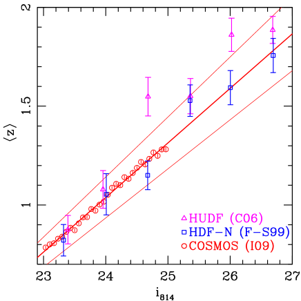
In order to include galaxies without individual photo-s in our analysis, we need to estimate their redshift distribution. Fig. 1 shows the mean photometric COSMOS-30 redshift for galaxies in our shear catalogue as a function of . In the whole magnitude range the data are very well described by the relation
| (1) |
For comparison we also plot points from the Hubble Deep Field-North (HDF-N, Fernández-Soto et al., 1999) and Hubble Ultra Deep Field (HUDF, Coe et al., 2006)444For the HUDF we interpolate from the and magnitudes provided in the Coe et al. (2006) catalogue. for the extended magnitude range , where both catalogues are redshift complete. The HDF-N data agree very well with the COSMOS fit over the whole extended range, on average to 2%. In contrast, the mean photometric redshifts in the HUDF are on average higher than (1) by 16% for and 10% for . The difference between the HDF-N and HUDF can be regarded as a rough estimate for the impact of sampling variance in such small fields. The fact that the HUDF galaxies systematically deviate from (1) not only for but also for where COSMOS-30 photo-s are available, indicates that it is most likely affected by sampling variance containing a relative galaxy over-density at higher redshift. Given the excellent fit for the COSMOS galaxies and very good agreement for the HDF-N data we are thus confident to use (1) for a limited extrapolation to for our shear galaxies. This is also motivated by the fact that and galaxies are not completely independent, but partially probe the same large-scale structure at different luminosities.
Due to the non-linear dependence of the shear signal on redshift it is not only necessary to estimate the correct mean redshift of the galaxies, but also their actual redshift distribution. In weak lensing studies the redshift distribution is often parametrized as (e.g. Brainerd et al., 1996), which Schrabback et al. (2007) extended by fitting in combination with a linear dependence of the median redshift on magnitude, leading to a magnitude-dependent . Yet, it was noted that this fit was not fully capable to reproduce the shape of the redshift distribution of the fitted galaxies. Given the higher accuracy needed for the analysis of the larger COSMOS data, we use a modified parametrization
| (2) |
where , and . Using a maximum likelihood fit555We employ the CERN Program Library MINUIT (http://wwwasdoc.web.cern.ch/wwwasdoc/minuit/). we determine best-fitting parameters from the individual magnitudes, photo-s, and (symmetric) 68% photo- errors of all galaxies with . From Eqs. (1) and (2) we then numerically compute the non-linear relation between and , for which we provide the fitting formulae
| (3) | |||||
| (4) |
with . The total redshift distribution of the survey is then simply given by the mean distribution .
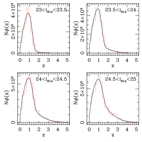
We chose the functional form of (2) because its first addend allows for a good description of the peak of the redshift distribution, while the second addend fits the magnitude-dependent tail at higher redshifts; see Fig. 2 for a comparison of the data and model in four magnitude bins.
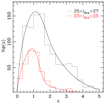
In Fig. 3 we compare the actual redshift distribution for the combined HDF-N and HUDF data to the one we predict from their magnitude distribution and the fit to the COSMOS data, finding very good agreement also for . The only major deviation is given by a galaxy over-density in the HUDF photo- data near , which is also partially responsible for the higher mean redshift in Fig. 1 and which may be attributed to large-scale structure.
Our fitting scheme assumes that the COSMOS-30 photo-s provide unbiased estimates for the true galaxy redshifts. However, in Sect. 2.2 we suspected that galaxies with assigned might contain a significant contamination with high-redshift galaxies. To assess the impact of this uncertainty, we derive the fits for (1) and (2) using only galaxies with , reducing the estimated mean redshift of shear galaxies without COSMOS-30 photo- by . As an alternative test, we assume that 20% of the galaxies with are truly at , increasing the estimated mean redshift by . Compared to the fit uncertainty in (1) () this constitutes the main source of error for our redshift extrapolation. In the cosmological parameter estimation (Sect. 6), we constrain this uncertainty and marginalize over it using a nuisance parameter, which rescales the redshift distribution within a conservatively chosen interval. Note that the difference between the measured and predicted mean redshift of the combined HDF-N and HUDF data in Fig. 3 actually suggests a smaller uncertainty.
3 Weak lensing shape measurements
To measure an accurate lensing signal, we have to carefully correct for instrumental signatures. Even with the high-resolution space-based data at hand, we have to accurately account for both PSF blurring and ellipticity, which introduce spurious shape distortions. To do so, one requires both a good model for the PSF, and a method which accurately employs it to measure unbiased estimates for the (reduced) gravitational shear from noisy galaxy images.
For the latter, we use the KSB+ formalism (Kaiser et al., 1995; Luppino & Kaiser, 1997; Hoekstra et al., 1998), see Erben et al. (2001); Schrabback et al. (2007) and App. B.1 for details on our implementation. As found with simulations of ground-based weak lensing data, KSB+ can significantly underestimate gravitational shear (Erben et al., 2001; Bacon et al., 2001; Heymans et al., 2006a; Massey et al., 2007a), where the calibration bias and possible PSF anisotropy residuals , defined via
| (5) |
depend on the details of the implementation. Massey et al. (2007a, STEP2) detected a shear measurement degradation for faint objects for our pipeline, which is not surprising given the fact that the KSB+ formalism does not account for noise. While Schrabback et al. (2007) simply corrected for the resulting mean calibration bias, the 3D weak lensing analysis performed here requires unbiased shape measurements not only on average, but also as function of redshift, and hence galaxy magnitude and size (see e.g. Kitching et al., 2008, 2009; Semboloni et al., 2009). We therefore empirically account for this degradation with a power-law fit to the signal-to-noise dependence of the calibration bias
| (6) |
where is computed with the galaxy size-dependent KSB weight function (Erben et al., 2001), and corrected for noise correlations as done in Hartlap et al. (2009). As relates to the significance of the galaxy shape measurement, it provides a more direct correction for noise-related bias than fits as a function of magnitude or size. We have determined this correction using the STEP2 simulations of ground-based weak lensing data (Massey et al., 2007a). In order to test if it performs reliably for the ACS data, we have analysed a set of simulated ACS-like data (see App. B.2). In summary, we find that the remaining calibration bias is on average, and over the entire magnitude range used, which is negligible compared to the statistical uncertainty for COSMOS. Likewise, PSF anisotropy residuals, which are characterized in (5) by , are found to be negligible in the simulation (dispersion ), assuming accurate PSF interpolation.
Weak lensing analyses usually create PSF models from the observed images of stars, which have to be interpolated for the position of each galaxy. Typically, a high galactic latitude ACS field contains only stars with sufficient , which are too few for the spatial polynomial interpolation commonly used in ground-based weak lensing studies. In addition, a stable PSF model cannot be used, given that substantial temporal PSF variations have been detected, mostly caused by focus changes resulting from orbital temperature variations (telescope breathing), mid-term seasonal effects, and long-term shrinkage of the optical telescope assembly (OTA) (e.g. Krist, 2003; Lallo et al., 2006; Anderson & King, 2006; Schrabback et al., 2007; Rhodes et al., 2007). To circumvent this problem, we have implemented a PSF correction scheme based on principal component analysis (PCA), as first suggested by Jarvis & Jain (2004). We have analysed 700 exposures of dense stellar fields, interpolated the PSF variation in each exposure with polynomials, and performed a PCA analysis of the polynomial coefficient variation. We find that of the total PSF ellipticity variation in random pointings can be described with a single parameter related to the change in telescope focus, confirming earlier results (e.g. Rhodes et al., 2007). However, we find that additional variations are still significant. In particular, we detect a dependence on the relative angle between the pointing and the orbital telescope movement666Technically speaking, we show a dependence on the velocity aberration plate scale factor in Fig. 21., suggesting that heating in the sunlight does not only change the telescope focus, but also creates slight additional aberrations dependent on the relative sun angle. These deviations may be coherent between COSMOS tiles observed under similar orbital conditions. To account for this effect, we split the COSMOS data into 24 epochs of observations taken closely in time, and determine a low-order, focus-dependent residual model from all stars within one epoch. We provide further details on our PSF correction scheme in App. B.5.
As an additional observational challenge, the COSMOS data suffer from defects in the ACS CCDs, which are caused by the continuous cosmic ray bombardment in space. These defects act as charge traps reducing the charge-transfer-efficiency (CTE), an effect referred to as charge-transfer-inefficiency (CTI). When the image of an object is transferred across such a defect during parallel read-out, a fraction of its charge is trapped and statistically released, effectively creating charge-trails following objects in the read-out -direction (e.g. Rhodes et al., 2007; Chiaberge et al., 2009; Massey et al., 2010). For weak lensing measurements the dominant effect of CTI is the introduction of a spurious ellipticity component in the read-out direction. In contrast to PSF effects, CTI affects objects non-linearly due to the limited depth of charge traps. Hence, the two effects must be corrected separately. As done by Rhodes et al. (2007), we employ an empirical correction for galaxy shapes, but also take the dependence on sky background into account. Making use of the CTI flux-dependence, we additionally determine and apply a parametric CTI model for stars, which is important as PSF and CTI-induced ellipticity get mixed otherwise. We present details on our CTI correction schemes for stars in App. B.4 and for galaxies in App. B.6. Note that Massey et al. (2010) recently presented a method to correct for CTI directly on the image level. We find that the methods employed here are sufficient for our science analysis, as also confirmed by the tests presented in Sect. 4. However, for weak lensing data with much stronger CTE degradation, such as ACS data taken after Servicing Mission 4, their pixel-based correction should be superior.
4 2D shear-shear correlations and tests for systematics
To measure the cosmological signal and conduct tests for systematics we compute the second-order shear-shear correlations
| (7) |
from galaxy pairs separated by . Here, if the galaxy separation falls within the considered angular bin around , and otherwise. In (7) we approximate our reduced shear estimates with the shear as commonly done in cosmological weak lensing (typically ; correction employed in Sect. 6.4), decompose it into the tangential component and the 45 degree rotated cross-component relatively to the separation vector, and employ uniform weights.
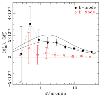
As an important consistency check in weak gravitational lensing, the signal can be decomposed into a curl-free component (E-mode) and a curl component (B-mode). Given that lensing creates only E-modes, the detection of a significant B-mode indicates the presence of uncorrected residual systematics in the data. Crittenden et al. (2002) show that can be decomposed into E- and B-modes as
| (8) |
with
| (9) |
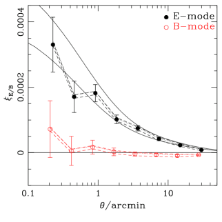
We plot this decomposition for our COSMOS catalogue in the left panel of Fig. 4. Given that the integration in (9) extends to infinity, we employ CDM predictions for , leading to a slight model-dependence, which is indicated by the dashed curves corresponding to , whereas the points have been computed for . Within this section, error-bars and covariances are estimated from 300 bootstrap resamples of our galaxy shear catalogue, which accounts for both shot noise and shape noise. As seen in Fig. 4, we detect no significant B-mode . However, note that different angular scales are highly correlated for , which mixes power on a broad range of scales and potentially smears out the signatures of systematics.
An E/B-mode decomposition, for which the correlation between different scales is weaker, is provided by the dispersion of the aperture mass (Schneider, 1996)
| (10) |
with given in Schneider et al. (2002), where we employ the aperture mass weight function proposed by Schneider et al. (1998). The computation of (10) requires integration from zero, which is not practical for real data. We therefore truncate for , where the introduced bias is small compared to our statistical errors (Kilbinger et al., 2006). Massey et al. (2007c) measure a significant B-mode component at scales , whereas this signal is negligible in the present analysis. We quantify the on average slightly positive by fitting a mean offset taking the bootstrap covariance into account (correlation between neighbouring points ), yielding an average if all points are considered, and or if only small scales are included, consistent with no B-modes.
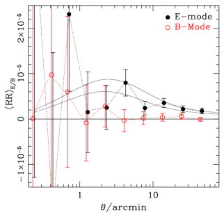
The cleanest E/B-mode decomposition is given by the ring statistics (Schneider & Kilbinger 2007; Eifler et al. 2009b; see also Fu & Kilbinger 2010), which can be computed from the correlation function using a finite interval with non-zero lower integration limit
| (11) |
with functions given in Schneider & Kilbinger (2007). We compute using a scale-dependent integration limit as outlined in Eifler et al. (2009b). As can be seen from the right panel of Fig. 4, also is consistent with no B-mode signal.
The non-detection of significant B-modes in our shear catalogue is an important confirmation for our correction schemes for instrumental effects and suggests that the measured signal is truly of cosmological origin.
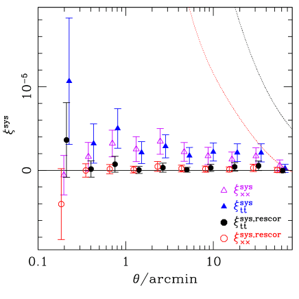
As a final test for shear-related systematics we compute the correlation between corrected galaxy shear estimates and uncorrected stellar ellipticities
| (12) |
which we normalize using the stellar auto-correlation as suggested by Bacon et al. (2003). As detailed in App. B.6, we employ a somewhat ad hoc residual correction for a very weak remaining instrumental signal. We find that is indeed only consistent with zero if this correction is applied (Fig. 5), yet even without correction, is negligible compared to the expected cosmological signal. The negligible impact can also be seen from the two-point statistics in Fig. 4, where the points are computed including residual correction, while the dotted lines indicate the measurement without it. We suspect that this residual instrumental signature could either be caused by the limited capability of KSB+ to fully correct for a complex space-based PSF, or a residual PSF modelling uncertainty due to the low number of stars per ACS field. In any case we have verified that this residual correction has a negligible impact on the cosmological parameter estimation in Sect. 6, changing our constraints on at the level, well within the statistical uncertainty.
5 Weak lensing tomography
In this section we present our analysis of the redshift dependence of the lensing signal in COSMOS. We start with the definition of redshift bins in Sect. 5.1, summarize the theoretical framework in Sect. 5.2, describe our angular binning and treatment of intrinsic galaxy alignments in Sect. 5.3, elaborate on the covariance estimation in Sect. 5.4, present the measured redshift scaling in Sect. 5.5, and discuss indications for a contamination of faint galaxies with high redshift galaxies in Sect. 5.6.
5.1 Redshift binning
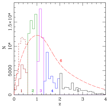
We split the galaxies with individual COSMOS-30 photo-s into five redshift bins, as summarized in Table 1 and illustrated in Fig. 6. We chose the intermediate limits such that the Balmer/4000Å break is approximately located at the centre of one of the broadband filters. This minimizes the impact of possible artifical clustering in photo- space and hence scatter between redshift bins for galaxies too faint to be detected in the Subaru medium bands. Given our chosen limits, most catastrophic redshift errors are faint bin 5 galaxies identified as bin 1 (Sect. 2.2.1). Thus, we do not include galaxies with in our analysis due to their potential contamination with high redshift galaxies, but study their lensing signal separately in Sect. 5.6. We use all galaxies without individual photo- estimates with 777Including galaxies with which are located in masked regions for the ground-based photo- catalogue, but not for the space-based lensing catalogue. as a broad bin 6, for which we estimated the redshift distribution in Sect. 2.2.2.
| Bin | ||||
|---|---|---|---|---|
| 1 | 0.0 | 0.6 | 22 294∗ | 0.37 |
| 29 817 | ||||
| 2 | 0.6 | 1.0 | 58 194 | 0.80 |
| 3 | 1.0 | 1.3 | 36 382 | 1.16 |
| 4 | 1.3 | 2.0 | 25 928 | 1.60 |
| 5 | 2.0 | 4.0 | 21 718 | 2.61 |
| 6 | 0.0 | 5.0 | 251 958 |
∗: Here we also exclude 259 galaxies with , which have a significant secondary peak in their redshift probability distribution at .
5.2 Theoretical description
Extending the formalism from Sect. 4, we split the galaxy sample into redshift bins and cross-correlate shear estimates between bins and
| (13) |
where the summation extends over all galaxies in bin , and all galaxies in bin . These are estimates for the shear cross-correlation functions , which are filtered versions of the convergence cross-power spectra
| (14) |
where denotes the -order Bessel function of the first kind and is the modulus of the two-dimensional wave vector. These can be calculated from line-of-sight integrals over the three-dimensional (non-linear) power spectrum (see Sect. 6.2) as
| (15) |
with the Hubble parameter , matter density , scale factor , comoving radial distance , comoving distance to the horizon , and comoving angular diameter distance . The geometric lens-efficiency factors
| (16) |
are weighted according to the redshift distributions of the two considered redshift bins (see e.g. Kaiser, 1992; Bartelmann & Schneider, 2001; Simon et al., 2004).
5.3 Angular binning and treatment of intrinsic galaxy alignments
Our six redshift bins define a total of 21 combinations of redshift bin pairs (including auto-correlations). For each redshift bin pair (), we compute the shear cross-correlations and in six logarithmic angular bins between 02 and . We include all of these angular and redshift bin combinations in the analysis of the weak lensing redshift scaling presented in this section, to keep it as general as possible. Yet, for the cosmological parameter estimation in Sect. 6, we carefully select the included bins to minimize potential bias by intrinsic galaxy alignments and uncertainties in theoretical model predictions.
In order to minimize potential contamination by intrinsic alignments of physically associated galaxies, we exclude the auto-correlations of the relatively narrow redshift bins 1 to 5. These contain the highest fraction of galaxy pairs at similar redshift, and hence carry the strongest potential contamination.
An additional contamination may originate from alignments between intrinsic galaxy shapes and their surrounding density field causing the gravitational shear (e.g. Hirata & Seljak, 2004; Hirata et al., 2007). A complete removal of this effect requires more advanced analysis schemes (e.g. Joachimi & Schneider, 2008), which we postpone to a future study. Yet, following the suggestion by Mandelbaum et al. (2006), we exclude luminous red galaxies (LRGs) in the computation of the shear-shear correlations used for the parameter estimation. This reduces potential contamination, given that LRGs were found to carry the strongest alignment signal (Mandelbaum et al., 2006, 2009; Hirata et al., 2007). We select these galaxies from the Ilbert et al. (2009) photo- catalogue with cuts in the photometric type (“ellipticals”) and absolute magnitude , excluding a total of 5 751 galaxies888In the cross-correlation between two redshift bins, it would be sufficient to exclude LRGs in the lower redshift bin only. However, for convenience we generally exclude them.. We accordingly adapt the redshift distribution for the parameter estimation.
In the cosmological parameter estimation, we additionally exclude the smallest angular bin (), for which the theoretical model predictions have the largest uncertainty due to required non-linear corrections (Sect. 6.2) and the influence of baryons (e.g. Rudd et al., 2008).
While we do not exclude LRGs and the smallest angular bin for the redshift scaling analysis presented in the current section, we have verified that their exclusion leads to only very small changes, which are well within the statistical errors and do not affect our conclusions.
5.4 Covariance estimation
In order to interpret our measurement and constrain cosmological parameters, we need to reliably estimate the data covariance matrix and its inverse. Massey et al. (2007c) estimate a covariance for their analysis from the variation between the four COSMOS quadrants. This approach yields too few independent realisations and may substantially underestimate the true errors (Hartlap et al., 2007). We also do not employ a covariance for Gaussian statistics (e.g. Joachimi et al., 2008) due to the neglected influence of non-Gaussian sampling variance. This is particularly important for the small-scale signal probed with COSMOS (Kilbinger & Schneider, 2005; Semboloni et al., 2007). Instead, we estimate the covariance matrix from 288 realisations of COSMOS-like fields obtained from ray-tracing through the Millennium Simulation (Springel et al., 2005), which combines a large simulated volume yielding many quasi-independent lines-of-sight with a relatively high spatial and mass resolution. The latter is needed to fully utilize the small-scale signal measureable in a deep space-based survey.
The details of the ray-tracing analysis are given in Hilbert et al. (2009). In brief, we use tilted lines-of-sight through the simulation to avoid repetition of structures along the backwards lightcone, providing us with quasi-independent fields, which we further subdivide into nine COSMOS-like subfields, yielding a total of 288 realisations. We randomly populate the fields with galaxies, employing the same galaxy number density, field masks, shape noise, and redshift distribution as in the COSMOS data. We incorporate photometric redshift errors for bins 1 to 5 by randomly misplacing galaxy redshifts assuming a (symmetric) Gaussian scatter according to the errors in the photo- catalogue. In contrast, the redshift calibration uncertainty for bin 6 is not a stochastic but a systematic error, which we account for in the cosmological model fitting in Sect. 6.
The value of used for the Millennium Simulation is slightly high compared to current estimates. This will lead to an overestimation of the errors, hence our analysis can be considered slightly conservative. We have to neglect the cosmology dependence of the covariance (Eifler et al., 2009a) in the parameter estimation, given that we have currently only one simulation with high resolution and large volume at hand.
We need to invert the covariance matrix for the cosmological parameter estimation in Sect. 6. While the covariance estimate from the ray-tracing realizations is unbiased, a bias is introduced by correlated noise in the matrix inversion. To obtain an unbiased estimate for the inverse covariance , we apply the correction
| (17) |
discussed in Hartlap et al. (2007), where is the number of independent realisations and is the dimension of the data vector. As discussed in Sect. 5.3, we exclude the smallest angular bin and auto-correlations of redshift bins 1 to 5, yielding and a moderate correction factor . In contrast, for the full data vector including all bins and correlations (), a very substantial correction factor would be required. Hence, our optimized data vector also leads to a more robust covariance inversion.
In order to limit the required correction for the covariance inversion, we do not include more angular bins in our analysis. We have therefore optimized the bin limits using Gaussian covariances (Joachimi et al., 2008) and a Fisher-matrix analysis aiming at maximal sensitivity to cosmological parameters.
5.5 Redshift scaling of shear-shear cross-correlations
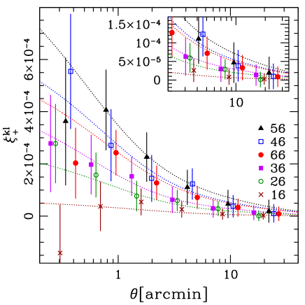
We plot the shear-shear cross-correlations between all redshift bins and the broad bin 6 in Fig. 7. These cross-correlations carry the lowest shot noise and shape noise due to the large number of galaxies in bin 6. The good agreement between the data and CDM model already indicates that the weak lensing signal roughly scales with redshift as expected. The errors correspond to the square root of the diagonal elements of the full ray-tracing covariance. Points are correlated not only within a redshift bin pair, but also between different redshift combinations, as their lensing signal is partially caused by the same foreground structures. In addition, galaxies in bin 6 contribute to different cross-correlations. Note that our relatively broad angular bins lead to a significant variation of the theoretical models within a bin. When computing an average model prediction for a bin, we therefore weight according to the -dependent number of galaxy pairs within this bin. Likewise, we plot points at their effective , which has been weighted accordingly.
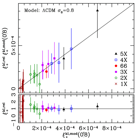
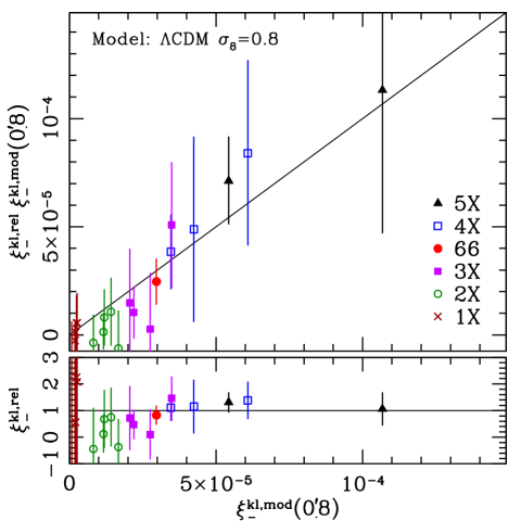
Instead of plotting 21 separation-dependent, noisy cross-correlations, we condense the information into a single plot showing the redshift dependence of the signal. Here we assume that the predictions for our reference cosmology describe the relative angular dependence of the signal sufficiently well, and fit the data points as
| (18) |
where is the model for the reference cosmology with , and is the fitted relative amplitude. In this fit, we take the full ray-tracing covariance between the angular scales into account. We plot the resulting 21 “collapsed” cross-correlations for both and in Fig. 8, as a function of their model prediction at a reference angular scale of 08, where points are again correlated. For both cases the redshift scaling of the signal is fully consistent with CDM expectations, showing a strong increase with redshift. This demonstrates that 3D weak lensing does indeed perform as expected. We note that for the signal is somewhat low for lower redshift combinations (smaller ), whereas it is slightly increased compared to predictions at higher redshifts. This behaviour is not surprising as most massive structures in COSMOS are located at (Scoville et al., 2007b), which create a lensing signal only for the higher redshift source bins. Slight differences between and are also expected, given that they probe the power spectrum with different filter functions, see Eq. (14).
5.6 Contamination of the excluded faint sample with high- galaxies
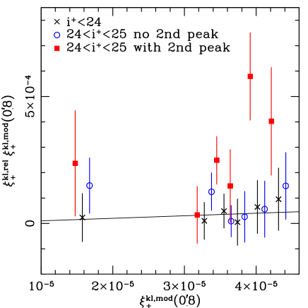
As discussed in Sect. 2.2, we expect a significant fraction of faint galaxies with assigned photometric redshift to be truly located at high redshifts . To test this hypothesis, we plot the collapsed shear cross-correlations for different samples of galaxies with assigned in Fig. 9. For the galaxies used in the cosmological analysis the signal is well consistent with expectations, suggesting negligible contamination. For a sample with single-peaked photo- probability distribution a mild increase is detected. This is still consistent with expectations, suggesting at most low contamination. We also study a sample of galaxies each of which has a significant secondary peak in their photometric redshift probability distribution at , amounting to 36% of all galaxies with . This sample shows a strong boost in the lensing signal, suggesting strong contamination with high-redshift galaxies.
We can obtain a rough estimate for this contamination if we assume that the shear signal does actually scale as in our reference CDM cosmology. For simplicity we assume that the cross-contamination can be described as a uni-directional scatter from bin 5 to bin 1, and that the true redshifts of the misplaced galaxies follow the distribution within bin 5. The expected contaminated signal is then given as a linear superposition of the cross-correlation predictions with bin 1 and bin 5 respectively, according to the relative number of contributing galaxy pairs
| (19) | |||||
where is the contamination fraction, i.e. the fraction of the bin 1 galaxies with and a significant secondary peak in their photo- PDF, which should have been placed into bin 5. We fit the measured shear-shear cross-correlations with (19) as a function of , where we fix the reference CDM cosmology and employ a special ray-tracing covariance (generated for ), yielding an estimate for the contamination , where the systematic error indicates the response to a change in by . This translates to a total contamination of for the galaxies with , which is consistent with our estimate for the redshift calibration uncertainty for bin 6 (Sect. 2.2.2). Note that we also measure an increased signal in for the sample with secondary photometric redshift peak, but do not include it in the fit (19) due to the stronger deviations for in Fig. 8. An adequate inclusion would then require a more complex analysis scheme, with a comparison not to the model predictions, but to all measured cross-correlations.
Our analysis provides an interesting confirmation for the photometric redshift analysis by Ilbert et al. (2009), which apparently succeeds in identifying sub-samples of (mostly) uncontaminated and potentially contaminated galaxies quite efficiently.
6 Constraints on cosmological parameters
6.1 Parameter estimation and considered cosmological models
The statistical analysis of the shear tomography correlation functions, assembled as data vector , is based on a standard Bayesian approach (e.g. MacKay, 2003). Therein, prior knowledge of model parameters is combined with the information on those parameters inferred from the new observation and expressed as posterior probability distribution function (PDF) of :
| (20) |
Here, is the prior based on theoretical constraints and previous observations, and denotes the evidence. The likelihood function is the statistical model of the measurement noise, for which we choose a Gaussian model
| (21) |
where is the parameter-dependent model, and the inverse covariance, which we estimated from the ray-tracing realizations in Sect. 5.4.
In our analysis we consider different cosmological models, which are characterized by the parameters , with the dark energy density , matter density , power spectrum normalization , Hubble parameter , and (constant) dark energy equation of state parameter . Here, denotes a nuisance parameter encapsulating the uncertainty in the redshift calibration for bin 6 as , which was discussed in Sect. 2.2.2. We consider
-
•
a flat CDM cosmology with fixed , , and ,
-
•
a general (non-flat) CDM cosmology with fixed and , , and
-
•
a flat CDM cosmology with , , and .
In all cases, we employ priors with flat PDFs for and . In our default analysis scheme we also apply a Gaussian prior for , and assume a fixed baryon density and spectral index as consistent with Dunkley et al. (2009), where the small uncertainties on and are negligible for our analysis. Note that we relax these priors for parts of the analysis in Sect. 6.3.2 and Sect. 6.4.
The practical challenge of the parameter estimation is to evaluate the posterior within a reasonable time, as the computation of one model vector for shear tomography correlations is time-intensive. For an efficient sampling of the parameter space, we employ the Population Monte Carlo (PMC) method as described in Wraith et al. (2009). This algorithm is an adaptive importance-sampling technique (Cappé et al., 2007): instead of creating a sample under the posterior as done in traditional Monte-Carlo Markov chain (MCMC) techniques (e.g. Christensen et al., 2001), points are sampled from a simple distribution, the so-called proposal, in our case a mixture of eight Gaussians. Each point is then weighted by the ratio of the proposal to the posterior at that point. In a number of iterative steps, the proposal function is adapted to give better and better approximations to the posterior. We run the PMC algorithm for up to eight iterations, using 5 000 sample points in each iteration. To reduce the Monte-Carlo variance, we use larger samples with 10 000 to 20 000 points for the final iteration. These are used to create density histograms, mean parameter values, and confidence regions. Depending on the experiment, the effective sample size of the final importance sample was between 7 500 and 17 700. We also cross-checked parts of the analysis with an independently developed code which is based on the traditional but less efficient MCMC approach, finding fully consistent results.
6.2 Non-linear power spectrum corrections
To calculate model predictions for the correlation functions according to (14), (15), and (16), we need to evaluate the involved distance ratios and compute the non-linear power spectrum . Given a set of parameter values, the computation of the distances and the linearly extrapolated power spectrum is straightforward. We employ the transfer function by Eisenstein & Hu (1998) for the latter, taking baryon damping but no oscillations into account (‘shape fit’).
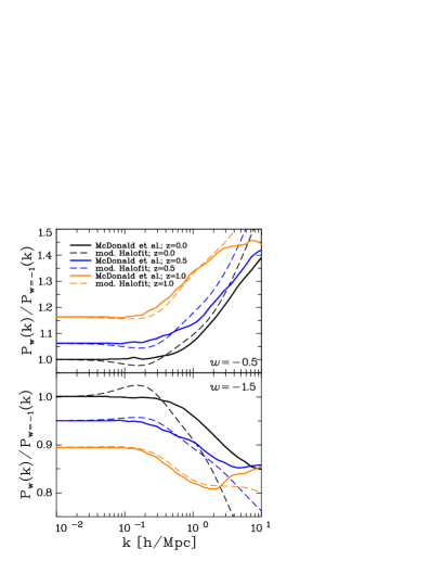
For CDM models we estimate the full non-linear power spectrum according to Smith et al. (2003). McDonald et al. (2006) also provide non-linear power spectrum corrections for , but these were tested for a narrow range in only. We want to keep our analysis as general as possible, not having to assume such a strong prior on . Following the icosmo code (Refregier et al., 2008) we instead interpolate the non-linear corrections from Smith et al. (2003) between the cases of a CDM cosmology () and an OCDM cosmology, acting as a dark energy with . This is achieved by replacing the parameter in the halo model fitting function (Smith et al., 2003). This parameter is used to interpolate between spatially flat models with dark energy () and an open Universe without dark energy (). We substitute by a new parameter . Thus, we obtain for CDM and for CDM with , mimicking an OCDM cosmology for which the original parameter vanished as well.
To test this simplistic approximation, we compare the computed corrections for to the fitting formulae from McDonald et al. (2006) in Fig. 10. Note that we use our fiducial cosmological parameters to obtain these curves, except for , to match from McDonald et al. (2006). For most of the scales probed by our measurement the two descriptions agree reasonably well. The modification of the halo fit follows the fits to the simulations more accurately on large scales and at higher redshift, while it does not reproduce the tendency of the fits by McDonald et al. (2006) to drop off for large wave vectors. The precision of the modification outlined above is sufficient for our aim to provide a proof of concept for weak lensing dark energy measurements. However, future measurements with larger data sets will require accurate fitting formulae for general cosmologies.
| Cosmology | Analysis | |||||
|---|---|---|---|---|---|---|
| Flat CDM | 3D | |||||
| Flat CDM | 2D | |||||
| General CDM | 3D | |||||
| Flat CDM | 3D |
6.3 Cosmological constraints from COSMOS
6.3.1 Flat CDM cosmology
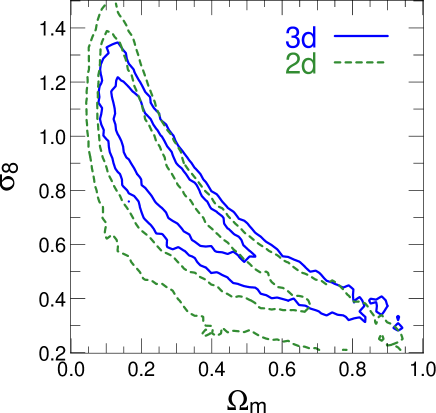
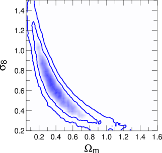
We plot our constraints on and for a flat CDM cosmology and our default 3D lensing analysis scheme in Fig. 11 (solid contours), showing the typical ’banana-shaped’ degeneracy, from which we compute999Here, we fit a power-law with slope minimizing the separation to all posterior-weighted points in the plane, and compute the 1D marginalized mean of within .
Here we marginalize over the uncertainties in and the parameter encapsulating the uncertainty in the redshift calibration for bin 6, where we find that is nearly uncorrelated with , and only weakly correlated with . The data allow us to weakly constrain , with a maximum posterior point at . This constraint is nearly unchanged for the other cosmological models considered below.
For comparison we also conduct a classic 2D lensing analysis (dashed contours in Fig. 11), where we use only the total redshift distribution and do not split galaxies into redshift bins. We find that the 2D and 3D analyses yield consistent results with substantially overlapping regions, as expected. Yet, the constraints from the 2D analysis shift towards lower . The difference is not surprising given that the strongest contribution to the lensing signal in COSMOS comes from massive structures near (Scoville et al., 2007b; Massey et al., 2007b), boosting the signal for high redshift sources, but leading to a lower signal for galaxies at low and intermediate redshifts (see right panel of Fig. 8). The 3D lensing analysis can properly combine these measurements, also accounting for the larger impact of sampling variance at low redshifts. In contrast, the 2D lensing analysis leads to a rather low (but still consistent) estimate for , due to the large number of low and intermediate redshift galaxies with low shear signal.
The tomographic analysis also reduces the degeneracy between and by probing the redshift-dependent growth of structure and distance-redshift relation, which differ substantially for a concordance CDM cosmology and e.g. an Einstein-de Sitter cosmology (). We summarize our parameter estimates in Table 2, also for the other cosmological models considered in the following subsections.
We also test our selection criteria for the optimized data vector (Sect. 5.3) by analysing several deviations from it for a flat CDM cosmology. We find negligible influence if the smallest angular scales or LRGs are included, suggesting that the measurement is robust regarding the influence of small-scale modelling uncertainties and intrinsic alignments between galaxy shapes and their surrounding density field. Performing the analysis using only the usually excluded auto-correlations of the relatively narrow redshift bins 1 to 5, we measure a slightly lower , which is still consistent given the substantially degraded statistical accuracy. If intrinsic alignments between physically associated galaxies contaminate the lensing measurement, we expect these auto-correlations to be most strongly affected. However, models predict an excess signal (e.g. Heymans et al., 2006b), whereas we measure a slight decrease within the statistical errors. Hence, we detect no significant indication for contamination by intrinsic galaxy alignments.
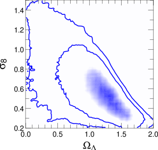
6.3.2 General (non-flat) CDM cosmology
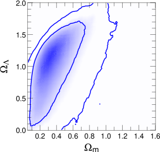
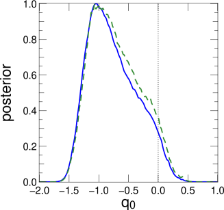
We plot our constraints for a general CDM cosmology without the assumption of flatness in Fig. 12. From the lensing data we find
where our prior excludes negative densities . Based on our constraints, we compute the posterior PDF for the deceleration parameter
| (22) |
as shown in Fig. 13, which yields
Relaxing our priors to (HST Key Project, Freedman et al., 2001), (Big-Bang nucleosynthesis, Iocco et al., 2009), and , weakens this constraint only slightly to
Employing the recent distance ladder estimate (Riess et al., 2009) instead of the HST Key Project constraint, we obtain at 94.8% confidence.
Our analysis provides evidence for the accelerated expansion of the Universe () from weak gravitational lensing. While the statistical accuracy is still relatively weak due to the limited size of the COSMOS field, this evidence is independent of external constraints on and .
We note that the lensing data alone cannot formally exclude a non-flat OCDM cosmology. However, the cosmological parameters inferred for such a model would be inconsistent with various other cosmological probes101010For a lensing-only OCDM analysis the posterior peaks at , (close to the prior boundaries). In the comparison with a CDM analysis, the additional parameter causes a penalty in the Bayesian model comparison (computed as in Kilbinger et al. 2009b). This leads to an only slightly larger evidence for the non-flat CDM model compared to the OCDM model, with an inconclusive evidence ratio of 65:35. The evidence ratio becomes a “weak preference” (77:23) if we employ a (still conservative) prior . Hence, with this prior the CDM model makes the data more than 3 times more probable than the OCDM model. . We therefore perform our analysis in the context of the well-established CDM model, where the lensing data provide additional evidence for cosmic acceleration.
6.3.3 Flat CDM cosmology
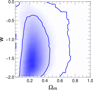
For a flat CDM cosmology we plot our constraints on the (constant) dark energy equation of state parameter in Fig. 14, showing that the measurement is consistent with CDM (). From the posterior PDF we compute
for the chosen prior . The exact value of this upper limit depends on the lower bound of the prior PDF given the non-closed credibility regions. We have chosen this prior as more negative would require a worrisome extrapolation for the non-linear power spectrum corrections (Sect. 6.2). For comparison, we repeat the analysis with a much wider prior leading to a stronger upper limit (). While the COSMOS data are capable to exclude very large values , larger lensing data-sets will be required to obtain really competitive constraints on .
To test the consistency of the data with CDM, we compare the Bayesian evidence for the flat CDM and CDM models, which we compute in the PMC analysis as detailed in Kilbinger et al. (2009b). Here we find completely inconclusive probability ratios for CDM versus CDM of () and (), confirming that the data are fully consistent with CDM.
6.4 Model recalibration with the Millennium Simulation and joint constraints with WMAP-5
Heitmann et al. (2008) and Hilbert et al. (2009) found that the Smith et al. (2003) fitting functions slightly underestimate non-linear corrections to the power spectrum. To test whether this has a significant influence on our results, we performed a 3D cosmological parameter estimation using the mean data vector of the 288 COSMOS-like ray-tracing realisations from the Millennium Simulation. Here we modify the strong priors given in Sect. 6.1 to match the input values of the simulation (, , , , ), and find 111111Here we have scaled the uncertainty for the mean ray-tracing data vector from the uncertainty for a single COSMOS-like field assuming that all realizations are completely independent. This is slightly optimistic given the large but finite volume of the simulation, and fact that the realizations were cut from larger fields. for . This confirms the result of Heitmann et al. (2008) and Hilbert et al. (2009), indicating that models based on Smith et al. (2003) slightly underestimate the shear signal, hence a larger is required to fit the data. Here we use actual reduced shear estimates from the simulation, but employ shear predictions, as done for the real data (see Sect. 4). Using shear estimates from the simulation yields . Hence, a minor contribution to the overestimation of is caused by the negligence of reduced shear corrections (see also Dodelson et al., 2006; Shapiro, 2009; Krause & Hirata, 2009).
To compensate for this underestimation of the model predictions and reduced shear effects, we scale our derived constraints on for a flat CDM cosmology by a factor 121212We expect that this correction factor depends on cosmological parameters. Yet, considering the weak lensing degeneracy for and , the input values of the Millennium Simulation are quasi equivalent to for , which is sufficiently close to our constraints to justify the application., yielding
Note that we did not apply this correction for the values given in the previous section and listed in Table 2, as we can only test it for the case of a flat CDM cosmology. Additionally, we want to keep the results comparable to previous weak lensing studies, which we expect to be similarly affected.
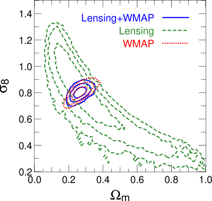
Having eliminated this last source of systematic uncertainty, we now estimate joint constraints with WMAP-5 CMB-only data (Dunkley et al., 2009), conducted similarly to the analysis by Kilbinger et al. (2009a). Here we assume a flat CDM cosmology, completely relax our priors to , , , and scale for the lensing model calculation according to the Millennium Simulation results. Here we also marginalize over an additional 2% uncertainty in the lensing calibration to account for the dropped remaining mean shear calibration bias (0.8%, Sect. 3) and limited accuracy of the employed residual shear correction (Sect. 4), which we estimate to be in . From the joint analysis with WMAP-5 we find
which reduces the size of WMAP-only () error-bars on average by (). We plot the joint and individual constraints in Fig. 15, illustrating the perfect agreement of the two independent cosmological probes.
7 Summary, discussion, and conclusions
We have measured weak lensing galaxy shear estimates from the HST/COSMOS data by applying a new model for the spatially and temporally varying ACS PSF, which is based on a principal component analysis of PSF variations in dense stellar fields. We find that most of the PSF changes can be described with a single parameter related to the HST focus position. Yet, we also correct for additional PSF variations, which are coherent for neighbouring COSMOS tiles taken closely in time. We employ updated parametric corrections for charge-transfer inefficiency, for both galaxies and stars, removing earlier modelling uncertainties due to confused PSF- and CTI-induced stellar ellipticity. Finally, we employ a simple correction for signal-to-noise dependent shear calibration bias, which we derive from the STEP2 simulations of ground-based weak lensing data. Tests on simulated space-based data confirm a relative shear calibration uncertainty over the entire used magnitude range if this correction is applied. We decompose the measured shear signal into curl-free E-modes and curl-component B-modes. As expected from pure lensing, the B-mode signal is consistent with zero for all second-order shear statistics, providing an important confirmation for the success of our correction schemes for instrumental systematics.
We combine our shear catalogue with excellent ground-based photometric redshifts from Ilbert et al. (2009) and carefully estimate the redshift distribution for faint ACS galaxies without individual photo-s. This allows us to study weak lensing cross-correlations in detail between six redshift bins, demonstrating that the signal indeed scales as expected from General Relativity for a concordance CDM cosmology.
We employ a robust covariance matrix from 288 simulated COSMOS-like fields obtained from ray-tracing through the Millennium Simulation (Hilbert et al., 2009). Using our 3D weak lensing analysis of COSMOS, we derive constraints for a flat CDM cosmology, using non-linear power spectrum corrections from Smith et al. (2003). A recalibration of these predictions based on the ray-tracing analysis changes our constraints to (all 68.3% conf.). Our results are perfectly consistent with WMAP-5, yielding joint constraints , (68.3% and 95.4% confidence). They also agree with weak lensing results from the CFHTLS-Wide (Fu et al., 2008) and recent galaxy cluster constraints from Mantz et al. (2009) within . Our errors include the full statistical uncertainty including the non-Gaussian sampling variance, Gaussian photo- scatter, and marginalization over remaining parameter uncertainties, including the redshift calibration for the faint galaxies.
Our results are consistent with the 3D lensing constraints from Massey et al. (2007c) assuming non-linear power spectrum corrections according to Smith et al. (2003), at the level. The analyses differ systematically in the treatment of PSF- and CTI-effects, where the success of our methods is confirmed by the vanishing B-mode. Furthermore, Massey et al. (2007c) employ earlier photo-s based on fewer bands (Mobasher et al., 2007). Note that the analysis of Massey et al. (2007c) yields tighter statistical errors, which may be a result of their covariance estimate from the variation between the four COSMOS quadrants. This potentially introduces a bias in the covariance inversion due to too few independent realisations (Hartlap et al., 2007). While the absolute calibration accuracy of the shear measurement method was estimated to be the dominant source of uncertainty in their error budget, we were able to reduce it well below the statistical error level. As a further difference, our analysis employs photometric redshift information to reduce potential contamination by intrinsic galaxy alignments, where we exclude the shear-shear auto-correlations for the relatively narrow redshift bins 1 to 5 to minimize the impact of physically associated galaxies. In addition, we exclude luminous red galaxies, which were found to carry the strongest intrinsic alignment with the density field of their large-scale structure environment causing the shear (Hirata et al., 2007). Finally, we do not include angular scales due to increased modelling uncertainties for the non-linear power spectrum.
Similarly to Massey et al. (2007c), we obtain a lower estimate for a non-tomographic (2D) analysis, assuming Smith et al. (2003) power spectrum corrections. The lower signal compared to the 3D lensing analysis is expected, given that the most massive structures in COSMOS are located at (Scoville et al., 2007b), creating a strong shear signal for high redshift sources only, which is detected by the 3D analysis. In contrast, the bulk of the galaxies in the 2D lensing analysis are located at too low redshifts to be substantially lensed by these structures, yielding a relatively low estimate for . Nonetheless, as sampling variance is properly accounted for in our error analysis, the constraints are still consistent.
For a general (non-flat) CDM cosmology, we find a negative deceleration parameter at 96.0% confidence using our default priors, and at 94.3% confidence if only priors from the HST Key Project and BBN are applied. Hence, our tomographic weak lensing measurement provides independent evidence for the accelerated expansion of the Universe. For a flat CDM cosmology we constrain the (constant) dark energy equation of state parameter to for a prior , fully consistent with CDM. Our dark energy constraints are still weak compared to recent results from independent probes (e.g. Kowalski et al., 2008; Hicken et al., 2009; Allen et al., 2008; Mantz et al., 2008, 2009; Vikhlinin et al., 2009; Komatsu et al., 2009). This is solely due to the limited area of COSMOS, leading to a dominant contribution to the error budget from sampling variance.
While the area covered by COSMOS is still small (1.64 ), the high resolution and depth of the HST data allowed us to obtain cosmological constraints which are comparable to results from substantially larger ground-based surveys. However, note that HST was by no means designed for cosmic shear measurements. In contrast, future space-based lensing mission such as Euclid131313http://sci.esa.int/euclid or JDEM141414http://jdem.gsfc.nasa.gov/ will be highly optimised for weak lensing measurements. High PSF stability, a much larger field-of-view providing thousands of stars for PSF measurements, carefully designed CCDs which minimize charge-transfer inefficiency, and improved algorithms will remove the need for some of the empirical calibrations employed in this paper.
In order to fully exploit the information encoded in the weak lensing shear field, second-order shear statistics, as used here, can be complemented with higher-order shear statistics to probe the non-Gaussianity of the matter distribution (e.g. Berge et al., 2009; Vafaei et al., 2010). Based on our COSMOS shear catalogue, Semboloni et al. (2010) present such a cosmological analysis using combined second and third-order shear statistics.
Finally, we stress that weak lensing can only provide precision constraints on cosmological parameters if sufficiently accurate models exist to compare the measurements to. Our analysis of the relatively small COSMOS Survey is still limited by the statistical measurement uncertainty, for which our approximate model recalibration using the Millennium Simulation is sufficient. Most of the cosmological sensitivity in COSMOS comes from quasi-linear and non-linear scales. We cut our analysis only at highly non-linear scales , corresponding to a comoving separation of kpc at (roughly the redshift of the most massive structures in COSMOS). At these scales non-linear power spectrum corrections have substantial uncertainties, in particular due to the influence of baryons (e.g. Rudd et al., 2008). Given that our results are basically unchanged if even smaller scales are included (insignificant increase in by ), we expect that the model uncertainty for the larger scales should still be sub-dominant compared to our statistical errors. However, analyses of large future surveys will urgently require improved model predictions including corrections for baryonic effects, also for dark energy cosmologies with , and optionally also for theories of modified gravity. Once these are available, careful analyses of large current and future weak lensing surveys will deliver precision constraints on cosmological parameters and dark energy properties.
Acknowledgements.
This work is based on observations made with the NASA/ESA Hubble Space Telescope, obtained from the data archives at the Space Telescope European Coordinating Facility and the Space Telescope Science Institute. It is a pleasure to thank the COSMOS team for making the Ilbert et al. (2009) photometric redshift catalogue publicly available. We appreciate help from Richard Massey and Jason Rhodes in the creation of the simulated space-based images. We thank them, Maaike Damen, Catherine Heymans, Karianne Holhjem, Mike Jarvis, James Jee, Alexie Leauthaud, Mike Lerchster, and Mischa Schirmer for useful discussions, and Steve Allen, Thomas Kitching, and Richard Massey for helpful comments on the manuscript. We thank the anonymous referee for his/her comments, which helped to improve this paper significantly. We thank the Planck-HFI and Terapix groups at IAP for support and computational facilities. TS acknowledges financial support from the Netherlands Organization for Scientific Research (NWO) and the Deutsche Forschungsgemeinschaft through SFB/Transregio 33 “The Dark Universe”. JH acknowledges support by the Deutsche Forschungsgemeinschaft within the Priority Programme 1177 under the project SCHN 342/6 and by the Bonn-Cologne Graduate School of Physics and Astronomy. BJ acknowledges support by the Deutsche Telekom Stiftung and the Bonn-Cologne Graduate School of Physics and Astronomy. MK is supported by the CNRS ANR “ECOSSTAT”, contract number ANR-05-BLAN-0283-04, and by the Chinese National Science Foundation Nos. 10878003 & 10778725, 973 Program No. 2007CB 815402, Shanghai Science Foundations and Leading Academic Discipline Project of Shanghai Normal University (DZL805). PSi, HHi, and MV acknowledge support by the European DUEL Research-Training Network (MRTN-CT-2006-036133). MB, CDF, and PJM acknowledge support from programs #HST-AR-10938 and #HST-AR-10676, provided by NASA through grants from the Space Telescope Science Institute (STScI), which is operated by the Association of Universities for Research in Astronomy, Incorporated, under NASA contract NAS5-26555 and NNX08AD79G. HHo and SH acknowledge support from a NWO Vidi grant. SH acknowledges support by the Deutsche Forschungsgemeinschaft within the Priority Programme 1177 under the project SCHN 342/6. ES acknowledges financial support from the Alexander von Humboldt Foundation. LVW thanks CIfAR and NSERC for financial support.Appendix A Additional image calibrations
In this appendix we describe additional calibrations which we apply to the flat-fielded _flt images before running MultiDrizzle.
Background subtraction.
We perform a quadrant-based background subtraction due to an anomalous bias level variation between the four ACS read-out amplifiers. Here we detect and mask objects with SExtractor (Bertin & Arnouts, 1996), combine this mask with the static bad pixel mask, and estimate the background as the median of all non-masked pixels in the quadrant. We modulate the offset from the mean background level with the normalised inverse flat-field to correct for the fact that the improperly bias-subtracted image has already been flat-fielded151515This procedure performs well for relatively empty fields such as the large majority of the COSMOS tiles. For fields dominated by a very bright star or galaxy, it can, however, lead to erroneous jumps in the background level. Hence, we generally adopt a maximal accepted difference in the background estimates of , which, if exceeded, leads to a subtraction of the minimum background estimate for all quadrants..
Bad pixel masking.
We manually mask satellite trails and scattered stellar light if its apparent sky position changes between different dither positions, allowing us to recover otherwise unusable sky area. In addition, we update the static bad pixel mask rejecting pixels if:
-
•
their dark current exceeds in the associated dark reference file (default ), or
-
•
they are affected by variable bias structures, which we identify in a variance image of five subsequent bias reference frames taken temporally close to the science frame considered, or
-
•
they show significantly positive or negative values in a median image computed from 50 background-subtracted and object-masked COSMOS frames taken closely in time, indicating any other semi-persistent blemish.
The latter two masks mainly aim at the rejection of variable bias structures which show up as positive or negative bad column segments in the stacked image if not properly masked. For the mask creation we utilize the IRAF task noao.imred.ccdmask. It computes the local median signal and rms variation in moving rectangles. A pixel is then masked if its values is either lsigma below or hsigma above the local median value. This is done for individual pixels and sums of pixels in column sections, where in the latter case the background dispersion is scaled by the square root of the number of pixels in the section. Finally each column is scanned for short segments of un-flagged pixels in between masked pixels. We additionally mask these segments if their length is less than 15 pixels. We summarise the values applied for the thresholds lsigma and hsigma in Table 3. Due to variations in image noise properties they do not perform optimally in all cases, so that we iteratively increase hsigma by if otherwise more than of the pixels in the bias variance image would be masked.
| Image type | lsigma | hsigma |
|---|---|---|
| Bias variance | 100 | 25, +5 if more than 2.5% masked |
| Median, gain=1 | 13 | 11 |
| Median, gain=2∗ | 15 | 15 |
∗: The COSMOS images were taken with , whereas the setting has been applied for some of the HAGGLeS fields (Marshall et al. 2010, in prep.). While we do not include these fields in the current analysis, they have been processed with the same pipeline upgrades described here. Hence, we list these values for completeness.
Noise model.
We compute a rms noise model for each pixel as
| (23) |
with the normalised flat-field , the sky background , the dark reference frame , the exposure time , the read-noise , and the bias variance image described in the previous paragraph, which requires scaling with the gain []. Containing all noise sources except object photon noise, this rms model is used for optimal pixel weighting in MultiDrizzle.
Appendix B Correction for PSF and CTI effects
B.1 Summary of our KSB+ implementation
We measure galaxy shapes using the Erben et al. (2001) implementation of the KSB+ formalism (Kaiser et al., 1995; Luppino & Kaiser, 1997; Hoekstra et al., 1998), as done in the earlier ACS weak lensing analysis of Schrabback et al. (2007). Object ellipticities161616We adopt the widely used term “ellipticity” here, but note that, strictly speaking, (24) corresponds to the definition of the polarisation.
| (24) |
are measured from weighted second-order brightness moments
| (25) |
where is a 2D Gaussian with dispersion . The response of a galaxy ellipticity to reduced gravitational shear and PSF effects is given by
| (26) |
with the (seeing convolved) intrinsic source ellipticity and the “pre-seeing” shear polarisability
| (27) |
where the shear and smear polarisability tensors and are calculated from higher-order brightness moments as detailed in Hoekstra et al. (1998). The PSF anisotropy kernel and ratio of and must be measured from stars and interpolated for each galaxy position, where we approximate the latter as .
In the application of the KSB+ formalism several choices lead to subtle differences between different KSB implementations, see Heymans et al. (2006a) for a detailed comparison. In short, we use sub-pixel interpolation for integral evaluations, measure galaxy shapes with , the SExtractor flux-radius, and apply PSF measurements computed with the same filter scale as used for the corresponding galaxy (interpolated between 24 values with pixels). We invert the tensor as measured from individual galaxies using the approximation commonly applied to reduce noise (Erben et al., 2001). In contrast to Schrabback et al. (2007) we do not apply a constant calibration correction, but employ the signal-to-noise dependent correction (6).
B.2 Tests with simulated space-based data
We test our KSB+ shape measurement pipeline on simulated space-based weak lensing data with ACS-like properties, which were provided for testing in the framework of the Shear Testing Programme171717http://www.physics.ubc.ca/~heymans/step.html. The images were created with the Massey et al. (2004) image simulation pipeline, which uses shapelets (Refregier & Bacon, 2003; Massey & Refregier, 2005) to model galaxy and PSF shapes, as already employed for the STEP2 simulations (Massey et al., 2007a). All images have pixels of size 004, HST-like resolution, and a depth equivalent to 2ks of ACS imaging. The data are subdivided into eight sets with different PSFs (), seven of which utilize TinyTim181818http://www.stsci.edu/software/tinytim/ ACS PSF models, and one was created by stacking stars of similar ellipticity in an ACS stellar field (M). One of the sets uses simplified exponential profiles for galaxy modelling (F), while the others include complex galaxy morphologies modelled with shapelets. Four sets comprise 100 images, while the others include 200 frames. Within each set, the images are split into “rotated pairs”, where the intrinsic galaxy ellipticities in one frame resemble 90 degree-rotated versions from the other frame, an approach used in Massey et al. (2007a) to reduce the analysis uncertainty due to shape-noise. Galaxies are sheared with and convolved with the PSF, both effects being constant within one frame, but with varying within one set. Realistic image noise was added similarly to the STEP2 analysis, except that no noise correlations were introduced.
We analyse the images with the same pipeline and cuts as the real COSMOS data, with the only difference that the PSF is assumed to be constant across the field, but still measured from the simulated stars. Fig. 16 shows the mean calibration bias and PSF anisotropy residuals defined in (5), separately for each image simulation set, estimated from matched galaxy pairs (for details on this fit see Massey et al., 2007a). While some data-sets deviate from the optimal , the residuals are at a level which is negligible compared to the statistical uncertainty of COSMOS. Combining all sets and both shear components, we estimate the mean calibration bias , and the scatter of the PSF anisotropy residuals .
As discussed in Sect. 3, a possible magnitude-dependence of the shear calibration bias is particularly problematic for 3D weak lensing studies. We therefore study as a function of magnitude in Fig. 17, both for the simulated ground-based STEP2 and the simulated space-based ACS-like data. Although the applied correction (6) was determined from the simulated ground-based data, it also performs very well for the ACS-like simulations, showing its robustness. Over the entire magnitude range the remaining calibration bias is , which is negligible compared to our statistical errors.
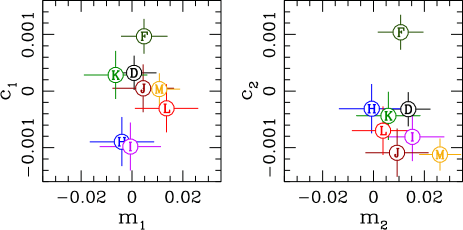

B.3 Stellar fields
We have analysed 700 exposures of dense stellar fields, which were taken between 2002 Apr 18 and 2006 Jun 03 and contain at least 300 non-saturated stars with (for pixels). This large set enables us to study in detail the impact of CTI on stars, as well as the temporal and positional ACS PSF variation, which cannot be achieved from the COSMOS exposures due to their low stellar density.
We determine both CTI and PSF models for the cosmic ray-cleansed COR images before resampling, and their resampled (but not stacked) counterparts (DRZ). The reason is that resampling unavoidably adds extra noise, hence it is best to fit the available stars in a galaxy field exposure before resampling. Yet, the combined PSF model for a stack has to be determined from resampled image models according to the relative dithering. For the COR-image analysis we employ a fixed Gaussian filter scale pixels, in order to maximize the fitting signal-to-noise (see Schrabback et al., 2007), and characterize the PSF by the ellipticity and stellar half-light radius as suggested by Jee et al. (2007). For the DRZ images we require CTI-corrected PSF models for all 24 values of used for the galaxy correction.
B.4 Stellar CTI correction
CTI charge trails stretch objects in the readout -direction, leading to an additional negative ellipticity component. Internal calibrations (Mutchler & Sirianni, 2005), photometric studies (e.g. Chiaberge et al., 2009), as well as the analysis of warm pixels (Massey et al., 2010) and cosmic rays (Jee et al., 2009) demonstrate that the influence of CTI increases linearly with time and the number of -transfers, where the latter has also been shown for the influence on galaxy ellipticities by Rhodes et al. (2007). In addition, the limited depth of charge traps leads to a stronger influence of CTI for faint sources, which lose a larger fraction of their charge than bright sources. Likewise, the effect is reduced for higher sky background values leading to a fraction of continuously filled traps. Here we only study the effect of CTI on stars, whereas galaxies will be considered in App. B.6.
Following Chiaberge et al. (2009), we assume a power-law dependence on sky background and integrated flux as measured in apertures of pixels, leading to the parametric CTI model
| (28) | |||||
with the time since the installation of ACS on 2002 Mar 08, and the number of -transfers . We expect that the normalisation and power law exponents and depend on the Gaussian filter scale of the KSB ellipticity measurement. E.g., for a measurement of the PSF core with small , charge traps may already be filled by electrons from the outer stellar profile, leading to an expected strong flux-dependence. On the contrary, the PSF wings measured at large will be more susceptible to trap filling by background electrons, leading to a stronger sky-dependence.
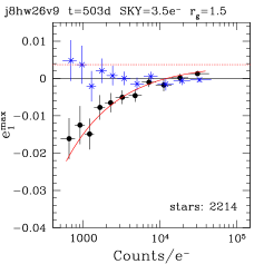
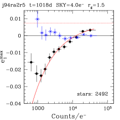
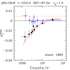
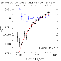
In order to separate CTI and PSF effects we make use of the fact that CTI-induced ellipticity is expected to depend on flux, while PSF ellipticity is flux-independent. In our analysis of stellar field exposures we first fit the spatial ellipticity variation of bright non-saturated stars with using a third-order polynomial in each chip, and apply this model to all stars with . For the high stars used in the fit, the strongest ellipticity contribution comes from the spatially varying PSF. Yet, for these stars the polynomial fit also corrects for the position-dependent but flux-averaged CTI effect, leading to a net negative ellipticity for fainter than average stars (CTI under-corrected), and net positive for brighter stars (CTI over-corrected). For even fainter stars with we expect an increasingly more negative ellipticity component. Hence, the CTI influence can be measured from the flux-dependence of the polynomial-corrected residual ellipticity, as illustrated in Fig. 18 for four example exposures. We note a turnaround in the CTI flux-dependence for some exposures at low (right panels in Fig. 18), which was also reported for CTI measurements from cosmic rays and further investigated by Jee et al. (2009). This does not affect our stellar models, given that we only use stars both for PSF measurement and to constrain (28). Yet, it suggests that CTI models may not be valid over very wide ranges in signal-to-noise, motivating the use of a separate model for the typically much fainter galaxies in App. B.6.
We determine the three fit parameters in (28) jointly from the polynomial-corrected residual ellipticities in all stellar exposures. For each exposure it is necessary to add an offset, which has been linearly scaled with for each star, in order to compensate for the flux-averaged correction included in the polynomial fit. We compute this offset within the non-linear fitting routine191919For the non-linear CTI fits we utilize the CERN Program Library MINUIT: http://wwwasdoc.web.cern.ch/wwwasdoc/minuit/ for a given set of fit parameters from the positions and fluxes of the bright stars used in the polynomial fit, and apply it to all stars.
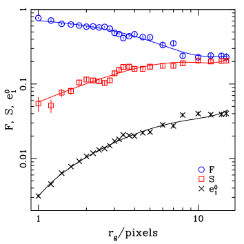
We conduct this fit both for the COR-image ellipticities () yielding best fitting values , and for the resampled DRZ-images for all values of . For the latter we adjust the cuts in order to keep enough stars for large . The best fit values are shown in Fig. 19 as function of , indeed confirming the expected trends. We provide the fitting functions
| (29) |
where the coefficients are listed in Table 4, being valid for pixels. We correct the ellipticities of all stars both in the stellar and galaxy fields with the derived models, as implicitly assumed in the following sections.
| 0 | |||
|---|---|---|---|
| 1 | |||
| 2 | |||
| 3 |
B.5 Principal component correction for the time-dependent ACS PSF
As discussed in Sect. 3, ACS PSF variations are expected to be mostly caused by changes in telescope focus (e.g. Krist, 2003; Lallo et al., 2006; Anderson & King, 2006). If the temporal variations indeed depend on one physical parameter only, it should be possible to construct a one-parametric PSF model, which can be well constrained with the stars available in an ACS field at high galactic latitudes. Such an approach was implemented by Rhodes et al. (2007), who measure the mean focus offset for a COSMOS stack from simulated focus-dependent TinyTim PSF models. They then interpolate the ACS PSF between all stars in COSMOS using polynomial functions dependent on both position and focus offset (Leauthaud et al., 2007; Massey et al., 2007c). However, as suggested by the residual aperture mass B-mode signal found by Massey et al. (2007c), this approach appears to be insufficient for a complete removal of systematics. In an alternative approach, Schrabback et al. (2007) fit the stars present in each galaxy field exposure using a large library of stellar field PSF models. While this approach led to no significant residual systematics within the statistical accuracy of GEMS, it is also not sufficient for the analysis of the much larger COSMOS data-set. We therefore implement a new PSF interpolation scheme based on principal component analysis. It effectively combines the idea of exposure-based empirical models, which optimally account for time variations and relative dithering (Schrabback et al., 2007), with the aim to describe the PSF variation with a single parameter (Rhodes et al., 2007).
Jarvis & Jain (2004) introduced the application of principal component analysis (PCA) for ground-based PSF interpolation, which we adapt here to obtain well-constrained PSF models for our ACS weak lensing fields. Note that Jee et al. (2007) and Nakajima et al. (2009) employed PCA to efficiently describe the two-dimensional ACS PSF shape, which they then spatially interpolated with normal polynomial functions. This is conceptually very different to the approach suggested by Jarvis & Jain (2004) and used here, which employs PCA for the spatial and temporal interpolation of certain quantities needed for PSF correction, such as the stellar ellipticity .
We represent all quantities which we want to interpolate as . This includes measured in the COR images for pixels, but also as measured in the DRZ images for varying . The only exception is when we specifically allude to COR quantities, which only includes the first group.
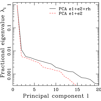
The first step of the PCA analysis is to fit the positional variation of the three COR PSF quantities in all stellar exposures jointly for both chips with 3rd-order polynomials
| (30) |
yielding coefficients each, where we generally denote polynomials using a capital with the order indicated by the superscript. Here we account for the gap between the chips and rescale the pixel range to the interval . While this fit is unable to account for some small-scale features such as a small discontinuity between the two chips, it captures all major large-scale PSF variations and is very well constrained by the required stars. For each exposure we arrange the polynomial coefficients in a data vector , with components (now ). We then subtract the mean vector and divide each component with an adequately chosen normalization , yielding the modified data vector with
| (31) |
We then arrange all modified data vectors into a dimensional data matrix . The central step of the PCA is a singular value decomposition , where the orthonormal matrix consists of the singular vectors of , and the diagonal matrix contains the ordered singular values of as diagonal elements. Here the th largest singular value corresponds to the th singular vector, which is also named the th principal component. In the coordinate system spanned by the singular vectors, the matrix corresponding to the covariance matrix for , becomes diagonal, where the sorted eigenvalues are equal to the variance of the vectors along the direction of the th principal component.
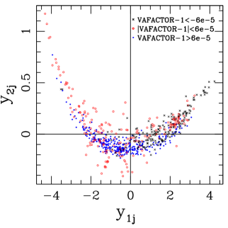
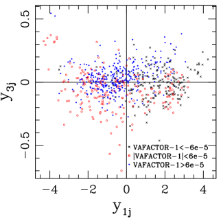
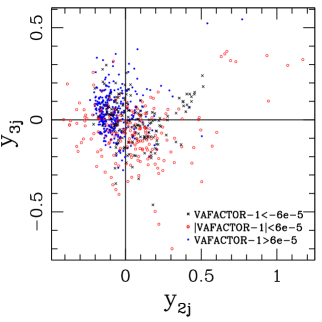
Note that the relative values and absolute scale of the eigenvalues depend on the normalisations . Uniform would not be adequate given that we combine PSF quantities with different units (dimensionless versus in pixels). A correlation analysis with could be used, but here relatively stable polynomial coefficients with small would unnecessarily add noise, effectively increasing the relative eigenvalues of higher principal components. Aiming at a compact description of most of the actual PSF variation in the field with a small number of important principal components, we employ the normalisation
| (32) |
where we use the mean variance of all coefficients belonging to the corresponding PSF quantity :
| (33) |
In this way the in (31) become dimensionless, all three PSF quantities contribute similarly to the total variation, and the undesired noise from relatively stable polynomial coefficients is avoided, as their variation is averaged with that from the less stable coefficients. The pre-factor in (32) equals the inverse of the integral of the corresponding polynomial term in (30). It accounts for our aim to scale according to the actual PSF variation, where e.g. a th-order term affects the whole field while a rd-order term with similar amplitude gets lower weight as it contributes substantially in a smaller area only.
We plot the fractional eigenvalues in Fig. 20, once using the analysis as described above (solid curve) and once considering only the two ellipticity components without (dashed curve). In both cases the first principal component is clearly dominant, contributing with () of the total variance. We identify this variation as the influence of focus changes, which are expected to dominate the actual PSF variation. The reason why the second principal component has a larger eigenvalue if is included in the analysis (fractional versus ) can be seen if we project the data variation onto the space spanned by the singular vectors , with components . Looking at the variation in the left panel of Fig. 21, where has been included, we see that the data points roughly follow a quadratic curve in the plane defined by the first two singular vectors. The reason for this is the linear response of PSF ellipticity on defocus caused by astigmatism, while PSF width responds to leading order quadratically (see e.g. Jarvis et al., 2008). Given that PCA is a purely linear coordinate transformation, it is not capable to directly capture this one-parametric variation (separation between primary and secondary mirror) with a single principal component. This is only possible if PSF quantities with the same dependence on physical parameters are included, hence the smaller if only the two ellipticity components are considered. Thus, for other applications it might be more favourable to perform a PCA analysis for each considered PSF quantity separately, as also done by Jarvis & Jain (2004). Yet, here we want to include the extra information encoded in the variation to constrain the galaxy field PSF models, and will therefore account for the non-linear dependence below. The mean stellar half-light radius in each exposure, is plotted as a function of the first principal component coefficient in Fig. 22, showing that a fourth-order polynomial fit is capable to describe the full non-linear variation.
In order to obtain a well constrained model for all with high spatial resolution, we jointly fit all stars from all exposures with a model
| (34) |
separately for both chips, where indicates a fifth-order polynomial in the corresponding rescaled , coordinates, and with and corresponds to the subtracted mean data vector, now modelled with high spatial resolution. We aim to fit the few stars in the galaxy fields with as few parameters as reasonably possible. Due to the dominant role of focus changes we hence use only the first principal component in our analysis , but include up to fourth-order terms () in . This takes out the non-linear distortion visible in Figs. 21 and 22, and hence the bulk of the variation in the second principal component. This combination yields a total of coefficients per PSF quantity and chip, which are very well constrained from a total of stars per chip.
For illustration we plot the field-of-view dependence of the high-resolution DRZ ellipticity model measured for pixels in Fig. 23, where the left panel shows the mean PSF ellipticity (), while the right panel depicts the first singular vector (). Note the slight discontinuity of the mean PSF ellipticity between the chips, which is likely caused by small height differences between the CCDs as reported by Krist (2003). See also Rhodes et al. (2007) who measure a stronger discontinuity in the TinyTim PSF model but not for stars in COSMOS, and Jee et al. (2007) who notice it in the PSF size but not ellipticity variation.
To obtain PSF models for our COSMOS stacks, we fit of all stars in the single COSMOS COR exposures with the PCA model (34) to determine the first principal component coefficient for this exposure. We then average the corresponding DRZ-image PSF models of all exposures contributing to a tile, taking their relative dither offsets and rotations into account, as detailed in Schrabback et al. (2007).
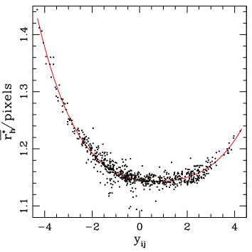
We plot the time dependence of the estimated coefficient for both the COSMOS and stellar field exposures in Fig. 24. Note that HST has been refocused at several occasions to compensate long-term shrinkage of the OTA, with one correction by microns being applied during the time-span of the COSMOS observations on 2004 Dec 22202020http://www.stsci.edu/hst/observatory/focus/ mirrormoves.html. To ease the comparison, all plots shown in Figs. 20 to 24 have been created using a single PCA model determined from all star fields. Yet, to exclude any possible influence of the refocusing, we actually use separate (but very similar) PCA models for the two epochs in our weak lensing analysis.
While the fit (34) captures of the total PSF variation in the stellar fields and metric defined above, it is important to realize that further PSF variations beyond focus changes do actually occur. These are indicated by the higher principal components and the additional scatter beyond the curved distortion in the second principal component. The subdivision of fields according to the velocity aberration plate scale factor VAFACTOR in Fig. 21, which depends on the angle between the pointing and the telescope orbital velocity vector (see e.g. Cox & Gilliland, 2002), indicates that these distortions are not random but may be coherent for neighbouring fields observed under similar conditions. This is not surprising given that HST undergoes substantial temperature changes and the relative angle towards the sun may lead to pointing-dependent effects212121Note that the actual impact of velocity aberration on object shapes is negligible for our analysis, as long as it is properly accounted for in the image stacking, as done by MultiDrizzle.. For a survey like COSMOS, where neighbouring fields have often been observed under similar conditions, we hence expect coherent residual PSF distortions beyond the one-parameter model introduced here.
These residuals cannot be constrained reliably from the few stars present in a single ACS galaxy field, as one would have to fit principal components given the slow decline of the eigenvalues (Fig. 20). However, under the assumption that they are semi-stable for fields observed under similar conditions, we can constrain these PSF residuals by combining the stars of multiple COSMOS tiles taken closely in time.


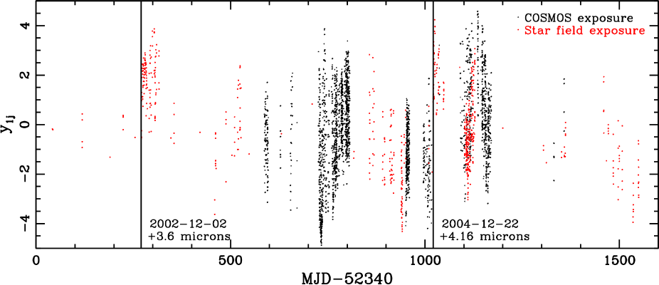
For this purpose, we split the COSMOS fields into 24 epochs. Within each epoch the data were taken closely in time, with the same orientation and similar sun angles. The only exception are two tiles which were reobserved between 2005 Oct 28 and 2005 Nov 24 due to previous guide-star failures (Koekemoer et al., 2007), which we add to epochs observed one year earlier under similar conditions. Within each epoch we combine the stars of all tiles and compute residuals of the DRZ image PSF quantities by correcting their values measured from the stacks with the (dithered and averaged) models (34). We then fit these residuals as
| (35) |
where has been averaged between the four exposures contributing to the stack , and and indicate second-order polynomials in the rescaled coordinates , determined for both chips together. Here we assume that the additional PSF variations are in principle stable during each epoch, but their impact might depend on the actual focus position and hence . Note that we do not use higher-order polynomials in , or non-linear powers of , as we would otherwise risk over-fitting for epochs with few contributing exposures. Yet, we tested slightly higher orders for those epochs containing sufficiently many stars, yielding nearly unchanged results. In general we found that the fitted coherent PSF residuals are small, with a mean rms model ellipticity of 0.3% (for pixels). However, some epochs showed somewhat enhanced ellipticity residuals, with two examples given in Fig. 25, motivating us to include this extra term in the galaxy PSF correction. In contrast we found that the residuals for are negligible. Also note that we deviate from our philosophy to obtain purely exposure-based models at this point, which is justified by the small and smooth (low-order) corrections applied, which are only marginally affected by dithering.


B.6 Galaxy correction and selection
We measure galaxy shapes and correct for PSF effects as detailed in the previous subsections. We then select galaxies with cuts , where is the maximum half-light radius of the pixel wide, automatically determined stellar locus in the image, , and , identical to the cuts applied to the simulated data in App. B.2. We also reject saturated stars and galaxies containing masked pixels (Sect. 2). In order to correct galaxy shapes for spurious CTI ellipticity, we fit the PSF anisotropy-corrected galaxy ellipticity component with the power law model
| (36) | |||||
with the mean sky level of the contributing exposures SKY, the time since the installation of ACS, the number of -transfers , the SExtractor flux-radius (FLUX_RADIUS), and the mean integrated flux per exposure measured by SExtractor. We scale the latter with the mean exposure time per exposure as the stacks are in units of . This model is similar to the one employed by Rhodes et al. (2007), but additionally accounts for the sky background-dependence of CTI effects and allows us to separate the dependence on galaxy flux and size. Despite the similarity to the stellar model (28), we do not determine a common CTI model for the typically bright stars and faint galaxies, as a simple power law fit is not guaranteed to work well over such a wide range in . Considering all selected COSMOS galaxies we determine best fitting parameters . The correction for field distortion leads to a mean rotation of the original -axis and hence readout direction in ACS stacks and DRZ exposures by . Thus, CTE degradation has also a minor effect on the ellipticity component, which we account for in both the galaxy and stellar correction as . Note that CTI affects an image after convolution with the PSF. Hence, one would ideally wish to correct for it first. Yet, in order to determine the impact of CTI, we need to correct for PSF anisotropy first, which would otherwise dominate the mean ellipticity. We then subtract the CTI model (36) and compute the fully corrected galaxy ellipticity with (26), which is an unbiased estimate for the shear if (5), (6) are taken into account. As it may be easier applicable for non-KSB methods, we also quote best-fitting parameters if the actual shear estimates are fitted instead of the PSF anisotropy-corrected ellipticities, where the difference is caused by the PSF seeing correction blowing up the CTI ellipticity.
As a test for residual instrumental signatures we create a stacked shear catalogue from all COSMOS tiles. Doing this, we marginally detect a very weak residual shear pattern, which changes with cuts on . To quantify and model this residual pattern, we fit it from the PSF anisotropy and CTI-corrected galaxy ellipticities with a focus-dependent, second-order model (35) jointly for all fields, yielding a very low rms ellipticity correction of . One possible explanation for these residuals could be the limited capability of KSB+ to fully correct for a complex space-based PSF, despite the very good performance on the simulated data in App. B.2. Alternatively the limited number of stars per field may ultimately limit the possible PSF modelling accuracy. In order to assess if these residuals have any significant impact on our results, we have performed our science analysis twice, once with and once without subtraction of this residual model. The resulting changes in our constraints on are at the level, which is negligible compared to the statistical uncertainties. Also the E/B-mode decomposition is nearly unchanged (Fig. 4). We only detect a significant influence for the star-galaxy cross-correlation, which is strictly consistent with zero only if this correction is applied, but even without correction it is negligible compared to the expected cosmological signal (Fig. 5).
As last step in the catalogue preparation, we create a joint mosaic shear catalogue from all fields, carefully rejecting double detections in neighbouring tiles, where we keep the detection with higher and refine relative shifts between tiles. In the case of close galaxy pairs with separations we exclude the fainter component. Our filtered shear catalogue contains 472 991 galaxies, corresponding to 80 galaxies, with a mean ellipticity dispersion per component . To limit the redshift extrapolation in Sect. 2.2.2, we apply an additional cut , leaving 446 934 galaxies, or 76 galaxies.
We rotate all shear estimates to common coordinates, and accordingly create a joint mosaic star catalogue for the analysis in Sect. 4.
References
- Albrecht et al. (2009) Albrecht, A., Amendola, L., Bernstein, G., et al. 2009, arXiv:0901.0721
- Albrecht et al. (2006) Albrecht, A., Bernstein, G., Cahn, R., et al. 2006, astro-ph/0609591
- Allen et al. (2008) Allen, S. W., Rapetti, D. A., Schmidt, R. W., et al. 2008, MNRAS, 383, 879
- Anderson (2007) Anderson, J. 2007, Instrument Science Rep. ACS 2007-08 (Baltimore: STScI), http://www.stsci.edu/hst/acs/documents/isrs/isr0708.pdf
- Anderson & King (2006) Anderson, J. & King, I. R. 2006, Instrument Science Rep. ACS 2006-01 (Baltimore: STScI), http://www.stsci.edu/hst/acs/documents/isrs/isr0601.pdf
- Bacon et al. (2000) Bacon, D., Refregier, A., & Ellis, R. 2000, MNRAS, 318, 625
- Bacon et al. (2003) Bacon, D. J., Massey, R. J., Refregier, A. R., & Ellis, R. S. 2003, MNRAS, 344, 673
- Bacon et al. (2001) Bacon, D. J., Refregier, A., Clowe, D., & Ellis, R. S. 2001, MNRAS, 325, 1065
- Bacon et al. (2005) Bacon, D. J., Taylor, A. N., Brown, M. L., et al. 2005, MNRAS, 363, 723
- Bartelmann & Schneider (2001) Bartelmann, M. & Schneider, P. 2001, Phys. Rep., 340, 291
- Benabed & Bernardeau (2001) Benabed, K. & Bernardeau, F. 2001, Phys. Rev. D, 64, 083501
- Benabed & van Waerbeke (2004) Benabed, K. & van Waerbeke, L. 2004, Phys. Rev. D, 70, 123515
- Benitez (2000) Benitez, N. 2000, ApJ, 536, 571
- Benjamin et al. (2007) Benjamin, J., Heymans, C., Semboloni, E., et al. 2007, MNRAS, 381, 702
- Berge et al. (2009) Berge, J., Amara, A., & Refregier, A. 2009, ApJ submitted (also arXiv:0909.0529)
- Bernstein & Jain (2004) Bernstein, G. & Jain, B. 2004, ApJ, 600, 17
- Bertin & Arnouts (1996) Bertin, E. & Arnouts, S. 1996, A&AS, 117, 393
- Brainerd et al. (1996) Brainerd, T., Blandford, R. D., & Smail, I. 1996, ApJ, 466, 623
- Bridle et al. (2010) Bridle, S., Balan, S. T., Bethge, M., et al. 2010, MNRAS accepted (also arXiv:0908.0945)
- Brown et al. (2003) Brown, M. L., Taylor, A. N., Bacon, D. J., et al. 2003, MNRAS, 341, 100
- Cappé et al. (2007) Cappé, O., Douc, R., Guillin, A., Marin, J.-M., & Robert, C. 2007, to appear in Statistics and Computing, also arXiv:0710.4242
- Chiaberge et al. (2009) Chiaberge, M., Lian Lim, P., Kozhurina-Platais, V., Sirianni, M., & Mack, J. 2009, Instrument Science Rep. ACS 2009-01 (Baltimore: STScI), http://www.stsci.edu/hst/acs/documents/isrs/isr0901.pdf
- Christensen et al. (2001) Christensen, N., Meyer, R., Knox, L., & Luey, B. 2001, Classical and Quantum Gravity, 18, 2677
- Coe et al. (2006) Coe, D., Benítez, N., Sánchez, S. F., et al. 2006, AJ, 132, 926
- Cox & Gilliland (2002) Cox, C. & Gilliland, R. L. 2002, in The 2002 HST Calibration Workshop. (Baltimore: STScI), p.58
- Crittenden et al. (2002) Crittenden, R. G., Natarajan, P., Pen, U.-L., & Theuns, T. 2002, ApJ, 568, 20
- de Bernardis et al. (2000) de Bernardis, P., Ade, P. A. R., Bock, J. J., et al. 2000, Nature, 404, 955
- Dodelson et al. (2006) Dodelson, S., Shapiro, C., & White, M. 2006, Phys. Rev. D, 73, 023009
- Doré et al. (2007) Doré, O., Martig, M., Mellier, Y., et al. 2007, Phys. Rev. D submitted (also arXiv:0712.1599)
- Dunkley et al. (2009) Dunkley, J., Komatsu, E., Nolta, M. R., et al. 2009, ApJS, 180, 306
- Eifler et al. (2009a) Eifler, T., Schneider, P., & Hartlap, J. 2009a, A&A, 502, 721
- Eifler et al. (2009b) Eifler, T., Schneider, P., & Krause, E. 2009b, A&A submitted (also arXiv:0907.2320)
- Eisenstein & Hu (1998) Eisenstein, D. J. & Hu, W. 1998, ApJ, 496, 605
- Eisenstein et al. (2005) Eisenstein, D. J., Zehavi, I., Hogg, D. W., et al. 2005, ApJ, 633, 560
- Erben et al. (2001) Erben, T., van Waerbeke, L., Bertin, E., Mellier, Y., & Schneider, P. 2001, A&A, 366, 717
- Fernández-Soto et al. (1999) Fernández-Soto, A., Lanzetta, K. M., & Yahil, A. 1999, ApJ, 513, 34
- Freedman et al. (2001) Freedman, W. L., Madore, B. F., Gibson, B. K., et al. 2001, ApJ, 553, 47
- Fu & Kilbinger (2010) Fu, L. & Kilbinger, M. 2010, MNRAS, 401, 1264
- Fu et al. (2008) Fu, L., Semboloni, E., Hoekstra, H., et al. 2008, A&A, 479, 9
- Giannantonio et al. (2008) Giannantonio, T., Scranton, R., Crittenden, R. G., et al. 2008, Phys. Rev. D, 77, 123520
- Granett et al. (2008) Granett, B. R., Neyrinck, M. C., & Szapudi, I. 2008, ApJ, 683, L99
- Hartlap et al. (2009) Hartlap, J., Schrabback, T., Simon, P., & Schneider, P. 2009, A&A, 504, 689
- Hartlap et al. (2007) Hartlap, J., Simon, P., & Schneider, P. 2007, A&A, 464, 399
- Heavens (2003) Heavens, A. 2003, MNRAS, 343, 1327
- Heavens et al. (2006) Heavens, A. F., Kitching, T. D., & Taylor, A. N. 2006, MNRAS, 373, 105
- Heitmann et al. (2008) Heitmann, K., White, M., Wagner, C., Habib, S., & Higdon, D. 2008, arXiv:0812.1052
- Hetterscheidt et al. (2007) Hetterscheidt, M., Simon, P., Schirmer, M., et al. 2007, A&A, 468, 859
- Heymans et al. (2005) Heymans, C., Brown, M. L., Barden, M., et al. 2005, MNRAS, 361, 160
- Heymans et al. (2006a) Heymans, C., Van Waerbeke, L., Bacon, D., et al. 2006a, MNRAS, 368, 1323
- Heymans et al. (2006b) Heymans, C., White, M., Heavens, A., Vale, C., & van Waerbeke, L. 2006b, MNRAS, 371, 750
- Hicken et al. (2009) Hicken, M., Wood-Vasey, W. M., Blondin, S., et al. 2009, ApJ, 700, 1097
- Hilbert et al. (2009) Hilbert, S., Hartlap, J., White, S. D. M., & Schneider, P. 2009, A&A, 499, 31
- Hildebrandt et al. (2009) Hildebrandt, H., Pielorz, J., Erben, T., et al. 2009, A&A, 498, 725
- Hildebrandt et al. (2008) Hildebrandt, H., Wolf, C., & Benítez, N. 2008, A&A, 480, 703
- Hirata et al. (2007) Hirata, C. M., Mandelbaum, R., Ishak, M., et al. 2007, MNRAS, 381, 1197
- Hirata & Seljak (2004) Hirata, C. M. & Seljak, U. 2004, Phys. Rev. D, 70, 063526
- Ho et al. (2008) Ho, S., Hirata, C., Padmanabhan, N., Seljak, U., & Bahcall, N. 2008, Phys. Rev. D, 78, 043519
- Hoekstra et al. (1998) Hoekstra, H., Franx, M., Kuijken, K., & Squires, G. 1998, ApJ, 504, 636
- Hoekstra & Jain (2008) Hoekstra, H. & Jain, B. 2008, Annual Review of Nuclear and Particle Science, 58, 99
- Hoekstra et al. (2006) Hoekstra, H., Mellier, Y., van Waerbeke, L., et al. 2006, ApJ, 647, 116
- Hoekstra et al. (2002) Hoekstra, H., Yee, H. K. C., & Gladders, M. D. 2002, ApJ, 577, 595
- Hu (1999) Hu, W. 1999, ApJ, 522, L21
- Hu (2002) Hu, W. 2002, Phys. Rev. D, 66, 083515
- Hu & Jain (2004) Hu, W. & Jain, B. 2004, Phys. Rev. D, 70, 043009
- Huterer (2002) Huterer, D. 2002, Phys. Rev. D, 65, 063001
- Huterer & Linder (2007) Huterer, D. & Linder, E. V. 2007, Phys. Rev. D, 75, 023519
- Ilbert et al. (2006) Ilbert, O., Arnouts, S., McCracken, H. J., et al. 2006, A&A, 457, 841
- Ilbert et al. (2009) Ilbert, O., Capak, P., Salvato, M., et al. 2009, ApJ, 690, 1236
- Iocco et al. (2009) Iocco, F., Mangano, G., Miele, G., Pisanti, O., & Serpico, P. D. 2009, Phys. Rep, 472, 1
- Jain & Taylor (2003) Jain, B. & Taylor, A. 2003, Physical Review Letters, 91, 141302
- Jain & Zhang (2008) Jain, B. & Zhang, P. 2008, Phys. Rev. D, 78, 063503
- Jarvis et al. (2003) Jarvis, M., Bernstein, G. M., Fischer, P., et al. 2003, AJ, 125, 1014
- Jarvis & Jain (2004) Jarvis, M. & Jain, B. 2004, ApJ submitted (also astro-ph/0412234)
- Jarvis et al. (2006) Jarvis, M., Jain, B., Bernstein, G., & Dolney, D. 2006, ApJ, 644, 71
- Jarvis et al. (2008) Jarvis, M., Schechter, P., & Jain, B. 2008, PASP submitted (also arXiv:0810.0027)
- Jee et al. (2007) Jee, M. J., Blakeslee, J. P., Sirianni, M., et al. 2007, PASP, 119, 1403
- Jee et al. (2009) Jee, M. J., Rosati, P., Ford, H. C., et al. 2009, ApJ, 704, 672
- Joachimi & Schneider (2008) Joachimi, B. & Schneider, P. 2008, A&A, 488, 829
- Joachimi et al. (2008) Joachimi, B., Schneider, P., & Eifler, T. 2008, A&A, 477, 43
- Kaiser (1992) Kaiser, N. 1992, ApJ, 388, 272
- Kaiser et al. (1995) Kaiser, N., Squires, G., & Broadhurst, T. 1995, ApJ, 449, 460
- Kaiser et al. (2000) Kaiser, N., Wilson, G., & Luppino, G. 2000, astro-ph/0003338
- Kilbinger et al. (2009a) Kilbinger, M., Benabed, K., Guy, J., et al. 2009a, A&A, 497, 677
- Kilbinger & Schneider (2005) Kilbinger, M. & Schneider, P. 2005, A&A, 442, 69
- Kilbinger et al. (2006) Kilbinger, M., Schneider, P., & Eifler, T. 2006, A&A, 457, 15
- Kilbinger et al. (2009b) Kilbinger, M., Wraith, D., Robert, C. P., et al. 2009b, MNRAS submitted (also arXiv:0912.1614)
- King & Schneider (2002) King, L. & Schneider, P. 2002, A&A, 396, 411
- Kitching et al. (2009) Kitching, T. D., Amara, A., Abdalla, F. B., Joachimi, B., & Refregier, A. 2009, MNRAS, 1430
- Kitching et al. (2007) Kitching, T. D., Heavens, A. F., Taylor, A. N., et al. 2007, MNRAS, 138
- Kitching et al. (2008) Kitching, T. D., Taylor, A. N., & Heavens, A. F. 2008, MNRAS, 389, 173
- Koekemoer et al. (2007) Koekemoer, A. M., Aussel, H., Calzetti, D., et al. 2007, ApJS, 172, 196
- Koekemoer et al. (2002) Koekemoer, A. M., Fruchter, A. S., Hook, R. N., & Hack, W. 2002, in The 2002 HST Calibration Workshop. Edited by S. Arribas, A. Koekemoer, and B. Whitmore. (Baltimore: STScI), p.337
- Komatsu et al. (2009) Komatsu, E., Dunkley, J., Nolta, M. R., et al. 2009, ApJS, 180, 330
- Kowalski et al. (2008) Kowalski, M., Rubin, D., Aldering, G., et al. 2008, ApJ, 686, 749
- Krause & Hirata (2009) Krause, E. & Hirata, C. M. 2009, A&A submitted (also arXiv:0910.3786)
- Krist (2003) Krist, J. 2003, Instrument Science Rep. ACS 2003-06 (Baltimore: STScI), http://www.stsci.edu/hst/acs/documents/isrs/isr0306.pdf
- Lallo et al. (2006) Lallo, M. D., Makidon, R. B., Casertano, S., & Krist, J. E. 2006, in Society of Photo-Optical Instrumentation Engineers (SPIE) Conference Series, Vol. 6270, Society of Photo-Optical Instrumentation Engineers (SPIE) Conference Series
- Leauthaud et al. (2007) Leauthaud, A., Massey, R., Kneib, J.-P., et al. 2007, ApJS, 172, 219
- Lilly et al. (2007) Lilly, S. J., Le Fèvre, O., Renzini, A., et al. 2007, ApJS, 172, 70
- Luppino & Kaiser (1997) Luppino, G. A. & Kaiser, N. 1997, ApJ, 475, 20
- MacKay (2003) MacKay, J. D. 2003, Information Theory, Inference, and Learning Algorithms (Cambridge University Press, Cambridge, UK)
- Mandelbaum et al. (2009) Mandelbaum, R., Blake, C., Bridle, S., et al. 2009, MNRAS submitted (also arXiv:0911.5347)
- Mandelbaum et al. (2006) Mandelbaum, R., Hirata, C. M., Ishak, M., Seljak, U., & Brinkmann, J. 2006, MNRAS, 367, 611
- Mantz et al. (2008) Mantz, A., Allen, S. W., Ebeling, H., & Rapetti, D. 2008, MNRAS, 387, 1179
- Mantz et al. (2009) Mantz, A., Allen, S. W., Rapetti, D., & Ebeling, H. 2009, MNRAS submitted (also arXiv:0909.3098)
- Massey et al. (2007a) Massey, R., Heymans, C., Bergé, J., et al. 2007a, MNRAS, 376, 13
- Massey & Refregier (2005) Massey, R. & Refregier, A. 2005, MNRAS, 363, 197
- Massey et al. (2005) Massey, R., Refregier, A., Bacon, D. J., Ellis, R., & Brown, M. L. 2005, MNRAS, 359, 1277
- Massey et al. (2004) Massey, R., Refregier, A., Conselice, C. J., David, J., & Bacon, J. 2004, MNRAS, 348, 214
- Massey et al. (2007b) Massey, R., Rhodes, J., Ellis, R., et al. 2007b, Nature, 445, 286
- Massey et al. (2007c) Massey, R., Rhodes, J., Leauthaud, A., et al. 2007c, ApJS, 172, 239
- Massey et al. (2010) Massey, R., Stoughton, C., Leauthaud, A., et al. 2010, MNRAS, 401, 371
- McDonald et al. (2006) McDonald, P., Trac, H., & Contaldi, C. 2006, MNRAS, 366, 547
- Miralles et al. (2005) Miralles, J.-M., Erben, T., Hämmerle, H., et al. 2005, A&A, 432, 797
- Mobasher et al. (2007) Mobasher, B., Capak, P., Scoville, N. Z., et al. 2007, ApJS, 172, 117
- Munshi et al. (2008) Munshi, D., Valageas, P., van Waerbeke, L., & Heavens, A. 2008, Phys. Rep, 462, 67
- Mutchler & Sirianni (2005) Mutchler, M. & Sirianni, M. 2005, Instrument Science Rep. ACS 2005-03 (Baltimore: STScI), http://www.stsci.edu/hst/acs/documents/isrs/isr0503.pdf
- Nakajima et al. (2009) Nakajima, R., Bernstein, G. M., Fadely, R., Keeton, C. R., & Schrabback, T. 2009, ApJ, 697, 1793
- Peacock et al. (2006) Peacock, J., Schneider, P., Efstathiou, G., et al. 2006, “Fundamental Cosmology”, ESA-ESO Working Groups Report No. 3 (also http://www.stecf.org/coordination/esa_eso/cosmology.php)
- Percival et al. (2007) Percival, W. J., Cole, S., Eisenstein, D. J., et al. 2007, MNRAS, 381, 1053
- Percival et al. (2009) Percival, W. J., Reid, B. A., Eisenstein, D. J., et al. 2009, MNRAS, 1741
- Perlmutter et al. (1999) Perlmutter, S., Aldering, G., Goldhaber, G., et al. 1999, ApJ, 517, 565
- Refregier et al. (2008) Refregier, A., Amara, A., Kitching, T., & Rassat, A. 2008, A&A submitted (also arXiv:0810.1285)
- Refregier & Bacon (2003) Refregier, A. & Bacon, D. 2003, MNRAS, 338, 48
- Refregier et al. (2002) Refregier, A., Rhodes, J., & Groth, E. J. 2002, ApJ, 572, L131
- Rhodes et al. (2004) Rhodes, J., Refregier, A., Collins, N. R., et al. 2004, ApJ, 605, 29
- Rhodes et al. (2007) Rhodes, J. D., Massey, R. J., Albert, J., et al. 2007, ApJS, 172, 203
- Riess et al. (1998) Riess, A. G., Filippenko, A. V., Challis, P., et al. 1998, AJ, 116, 1009
- Riess et al. (2009) Riess, A. G., Macri, L., Casertano, S., et al. 2009, ApJ, 699, 539
- Riess et al. (2007) Riess, A. G., Strolger, L.-G., Casertano, S., et al. 2007, ApJ, 659, 98
- Rudd et al. (2008) Rudd, D. H., Zentner, A. R., & Kravtsov, A. V. 2008, ApJ, 672, 19
- Schimd et al. (2007) Schimd, C., Tereno, I., Uzan, J., et al. 2007, A&A, 463, 405
- Schlegel et al. (1998) Schlegel, D. J., Finkbeiner, D. P., & Davis, M. 1998, ApJ, 500, 525
- Schmidt (2008) Schmidt, F. 2008, Phys. Rev. D, 78, 043002
- Schneider (1996) Schneider, P. 1996, MNRAS, 283, 837
- Schneider (2006) Schneider, P. 2006, in: Gravitational Lensing: Strong, Weak & Micro, Saas-Fee Advanced Course 33, Swiss Society for Astrophysics and Astronomy, G. Meylan, P. Jetzer & P. North (Eds.), Springer-Verlag: Berlin, p. 269
- Schneider & Kilbinger (2007) Schneider, P. & Kilbinger, M. 2007, A&A, 462, 841
- Schneider et al. (1998) Schneider, P., van Waerbeke, L., Jain, B., & Kruse, G. 1998, MNRAS, 296, 873
- Schneider et al. (2002) Schneider, P., van Waerbeke, L., & Mellier, Y. 2002, A&A, 389, 729
- Schrabback et al. (2007) Schrabback, T., Erben, T., Simon, P., et al. 2007, A&A, 468, 823
- Scoville et al. (2007a) Scoville, N., Abraham, R. G., Aussel, H., et al. 2007a, ApJS, 172, 38
- Scoville et al. (2007b) Scoville, N., Aussel, H., Benson, A., et al. 2007b, ApJS, 172, 150
- Semboloni et al. (2006) Semboloni, E., Mellier, Y., van Waerbeke, L., et al. 2006, A&A, 452, 51
- Semboloni et al. (2010) Semboloni, E., Schrabback, T., Van Waerbeke, L., et al. 2010, MNRAS submitted
- Semboloni et al. (2009) Semboloni, E., Tereno, I., van Waerbeke, L., & Heymans, C. 2009, MNRAS, 397, 608
- Semboloni et al. (2007) Semboloni, E., van Waerbeke, L., Heymans, C., et al. 2007, MNRAS, 375, L6
- Shapiro (2009) Shapiro, C. 2009, ApJ, 696, 775
- Simon et al. (2004) Simon, P., King, L. J., & Schneider, P. 2004, A&A, 417, 873
- Smith et al. (2003) Smith, R. E., Peacock, J. A., Jenkins, A., et al. 2003, MNRAS, 341, 1311
- Spergel et al. (2003) Spergel, D. N., Verde, L., Peiris, H. V., et al. 2003, ApJS, 148, 175
- Springel et al. (2005) Springel, V., White, S. D. M., Jenkins, A., et al. 2005, Nature, 435, 629
- Suyu et al. (2009) Suyu, S. H., Marshall, P. J., Auger, M. W., et al. 2009, ApJ submitted (also arXiv/0910.2773)
- Takada & Jain (2004) Takada, M. & Jain, B. 2004, MNRAS, 348, 897
- Taylor et al. (2007) Taylor, A. N., Kitching, T. D., Bacon, D. J., & Heavens, A. F. 2007, MNRAS, 374, 1377
- Vafaei et al. (2010) Vafaei, S., Lu, T., van Waerbeke, L., et al. 2010, Astroparticle Physics, 32, 340
- Van Waerbeke et al. (2000) Van Waerbeke, L., Mellier, Y., Erben, T., et al. 2000, A&A, 358, 30
- Van Waerbeke et al. (2005) Van Waerbeke, L., Mellier, Y., & Hoekstra, H. 2005, A&A, 429, 75
- Vikhlinin et al. (2009) Vikhlinin, A., Kravtsov, A. V., Burenin, R. A., et al. 2009, ApJ, 692, 1060
- Wittman et al. (2000) Wittman, D. M., Tyson, J. A., Kirkman, D., Dell’Antonio, I., & Bernstein, G. 2000, Nature, 405, 143
- Wraith et al. (2009) Wraith, D., Kilbinger, M., Benabed, K., et al. 2009, Phys. Rev. D, 80, 023507