Observation of Anti-correlation of Classical Chaotic Light

Abstract

We wish to report an experimental observation of anti-correlation from first-order incoherent classical chaotic light. We explain why the classical statistical theory does not apply and provide a quantum interpretation. In quantum theory, either correlation or anti-correlation is a two-photon interference phenomenon, which involves the superposition of two-photon amplitudes, a nonclassical entity corresponding to different yet indistinguishable alternative ways of producing a joint-photodetection event.

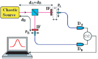
In 1956, Hanbury Brown and Twiss (HBT) discovered a nontrivial intensity correlation in thermal light HBT . Figure 1 schematically illustrates a modern HBT interferometer or the so called “intensity interferometer”. In a temporal HBT interferometer, the temporal, randomly distributed, chaotic thermal light has a twice greater chance of being measured within its coherence time by the joint-detection of two individual photodetectors. In a spatial HBT interferometer, the spatial, randomly distributed, chaotic thermal light exhibits a twice greater chance of being captured within a small transverse area that equals the spatial coherence of the thermal radiation by two point photodetectors . It was recently found that for a large angular sized chaotic source the spatial correlation is effectively within a physical “point”. The point-to-point near-field spatial correlation of chaotic light has been utilized for reproducing nonlocal ghost images in a lensless configuration Gpaper .

Figure 1: Schematic of a modern HBT interferometer which measures both temporal and spatial correlation of light by scanning the optical fiber tips longitudinally or transversely.

What is the physical cause of this peculiar behavior of chaotic thermal light? In the classical point of view, the HBT phenomenon is a statistical correlation of intensity fluctuations of thermal radiation. In general, no matter how complicated the optical setup is, classical theory considers the joint-detection between two individual, point-like photodetectors, $D_{A}$ and $D_{B}$, as a measure of the statistical correlation of two intensities at space-time coordinates $(\mathbf{r}_{A},t_{A})$ and $(\mathbf{r}_{B},t_{B})$

$$\ \ \ \ \Gamma^{(2)}(\mathbf{r}_{A},t_{A};\mathbf{r}_{B},t_{B})=\langle I(\mathbf{r}_{A},t_{A})\,I(\mathbf{r}_{B},t_{B})\rangle$$ (1)

$$=\langle I(\mathbf{r}_{A},t_{A})\rangle\langle I(\mathbf{r}_{B},t_{B})\rangle+\langle\Delta I(\mathbf{r}_{A},t_{A})\,\Delta I(\mathbf{r}_{B},t_{B})\rangle.$$

The HBT observation comes from the second term of Eq. (1), which indicates correlated intensity fluctuations at a distance. Why do the two distant intensities fluctuate in such a peculiar manner? One historical answer is “photon bunching”, i.e., a thermal light source has a higher chance of emitting photons in pairs. Another involves the coherence of the electromagnetic fields

$$\ \ \ \ \Gamma^{(2)}(\mathbf{r}_{A},t_{A};\mathbf{r}_{B},t_{B})=\langle I(\mathbf{r}_{A},t_{A})\,I(\mathbf{r}_{B},t_{B})\rangle$$

$$=\langle E^{*}(\mathbf{r}_{A},t_{A})E(\mathbf{r}_{A},t_{A})E^{*}(\mathbf{r}_{B},t_{B})E(\mathbf{r}_{B},t_{B})\rangle$$

$$=\Gamma^{(1)}_{AA}\Gamma^{(1)}_{BB}+\Gamma^{(1)}_{AB}\Gamma^{(1)}_{BA},$$ (2)

where $\Gamma^{(1)}_{jj}=\langle E^{*}(\mathbf{r}_{j},t_{j})E(\mathbf{r}_{j},t_{j})\rangle=\langle I(\mathbf{r}_{j},t_{j})\rangle$, $j=A,B$, is defined as the self-coherence function, or self-correlation function of the field; $\Gamma^{(1)}_{AB}=\Gamma^{*(1)}_{BA}=\langle E^{*}(\mathbf{r}_{A},t_{A})E(\mathbf{r}_{B},t_{B})\rangle$ is defined as the mutual-coherence, or mutual-correlation function of the field. It has been well accepted that an intensity-interferometer measures the mutual-correlation $\Gamma^{(1)}_{AB}$ of the input field, no matter how complicated the optical setup.

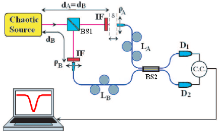
Figure 2: Schematic setup of the experiment.

Now we consider a slightly different experimental setup in Fig. 2. Instead of directly measuring the intensity correlation of $\langle I(\mathbf{r}_{A},t_{A})\,I(\mathbf{r}_{B},t_{B})\rangle$, this setup measures $\langle I(\mathbf{r}_{1},t_{1})\,I(\mathbf{r}_{2},t_{2})\rangle$ at the output ports of a $50/50$ optical fiber beamsplitter. If the two input fiber tips A and B are placed within the longitudinal coherence time and the transverse coherence area of the thermal field, this setup is equivalent to a Mach-Zehnder interferometer. $D_{1}$ and $D_{2}$ will each measure first-order interference as a function of the optical delay $\delta$ when scanning the fiber tip A along its longitudinal axis. Consequently, the joint-detection of $D_{1}$ and $D_{2}$ outputs an interference pattern that is factorizable into two first-order interferences. However, this is not our desired experimental condition. We decided to move the fiber tip A outside the transverse coherence area to force $\Gamma^{(1)}_{AB}=0$. Under this condition, there would be no observable first-order interference in a timely averaged measurement and in a instantaneous “single-exposure” observation Mandel . Consequently, the standard classical statistical correlation theory of intensity fluctuations gives the following second-order correlation $\Gamma^{(2)}$ that is independent of optical delay $\delta$,

$$\ \ \ \ \Gamma^{(2)}(\mathbf{r}_{1},t_{1};\mathbf{r}_{2},t_{2})=\langle I(\mathbf{r}_{1},t_{1})\,I(\mathbf{r}_{2},t_{2})\rangle$$ (3)

$$=\langle\big{|}E(\mathbf{r}_{A},t_{1A})+E(\mathbf{r}_{B},t_{1B})\big{|}^{2}\big{|}E(\mathbf{r}_{A},t_{2A})-E(\mathbf{r}_{B},t_{2B})\big{|}^{2}\rangle,$$

where $(\mathbf{r}_{A},t_{jA}=t_{j}-r_{Aj}/c)$ and $(\mathbf{r}_{B},t_{jB}=t_{j}-r_{Bj}/c$), $j=1,2$, with $r_{Aj}/c$ ($r_{Bj}/c$) the optical delay from point A (B) to $D_{j}$, are earlier space-time coordinates at points $A$ and $B$. In the Appendix A we show in detail why the classical statistical intensity correlation $\Gamma^{(2)}(\mathbf{r}_{1},t_{1};\mathbf{r}_{2},t_{2})$ is $\delta$ independent. In fact, the physics is rather simple; mathematically Eq. (3) has sixteen terms to begin with. However, all $\Gamma^{*(1)}_{AB}\Gamma^{(1)}_{AB}$ terms vanish due to the mutual incoherence between fields $E(\mathbf{r}_{A},t_{A})$ and $E(\mathbf{r}_{B},t_{B})$, leaving only these nonzero terms which have no contribution from the $\delta$-dependent first-order mutual coherence.

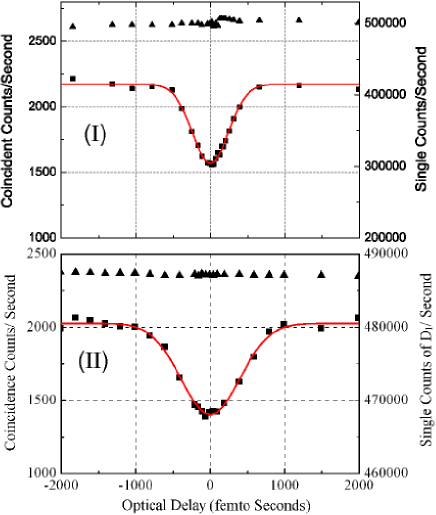
The measurement produces quite a surprise. A “unexpected” anti-correlation “dip” was observed in the joint-detection counting rate of $D_{1}$ and $D_{2}$ as a function of the optical delay $\delta$. Figure 3 reports two typical measured anti-correlation functions with different spectrum bandwidths of the chaotic field.

Figure 3: Two typical observed anti-correlation functions with different coherence time of the chaotic field. $\tau_{c}\sim 345fs$ for (I), $\tau_{c}\sim 541fs$ for (II). The coherence time is determined by the bandwidth of the spectral filters (IF).

The experimental detail is described as follows.

(1) The source: the light source is a standard pseudo-thermal source that was developed in the 1960’s and used widely in HBT correlation measurements Pseudo . The source consists of a CW mode-locked laser beam with $\sim$200 femtosecond pulses at a 78 MHz repetition rate and a fast rotating diffusing ground glass. The linearly polarized laser beam is enlarged transversely onto the ground glass with a diameter of $4.5mm$. The enlarged laser radiation is scattered and diffused by the rotating ground glass to simulate a near-field, chaotic-thermal radiation source: a large number of independent point sub-sources with independent, random, relative phases.

(2) The interferometer: A 50/50 beam splitter (BS1) is used to split the chaotic light into transmitted and reflected radiations which are then coupled into two identical polarization-controlled single-mode fibers A and B respectively. The fiber tips are located $\sim 200mm$ from the ground glass, i.e. $d_{A}=d_{B}\sim 200mm$. At this distance, the angular size $\Delta\theta$ is $\sim 22.5$ mili-radian ($1.29^{\circ}$) with respect to each input fiber tip, which satisfies the Fresnel near-field condition. Two identical narrow-band spectral filters (IF) are placed in front of the two fiber tips A and B. The transverse and longitudinal coordinates of the input fiber tips are both scannable by step-motors. The output ends of the two fibers can be directly coupled into the photon counting detectors $D_{1}$ and $D_{2}$, respectively, for near-field HBT correlation measurements, or coupled into the two input ports of a 50/50 single-mode optical fiber beamsplitter(BS2) for the anti-correlation measurement.

(3) The measurement: two steps of measurements were made. The purpose of step one is to confirm the light source produces chaotic-thermal field. We measured the HBT temporal and spatial correlation by scanning the input fiber tips longitudinally and transversely. In this measurement the output ends of the fibers are coupled into $D_{A}$ and $D_{B}$ directly as shown in Fig. 1. Chaotic radiation can easily be distinguished from a laser beam by examining its second-order coherence function $G^{(2)}(\mathbf{r}_{A},t_{A};\mathbf{r}_{B},t_{B})$, which is characterized experimentally by the coincidence counting rate that counts the joint photo-detection events at space-time points $(\mathbf{r}_{A},t_{A})$ and $(\mathbf{r}_{B},t_{B})$.

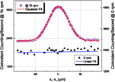
Figure 4: Measurement of $G^{(2)}(x_{A}-x_{B})$ at no rotation(0 rpm) and at 1000 rpm. Here, $x_{A}$ and $x_{B}$ are the x-component of $\vec{\rho}_{A}$ and $\vec{\rho}_{B}$, and correspondingly y components are kept $y_{A}=y_{B}$.

Figure 4 reports two measured second-order correlations at zero and at 1000 revolutions per minute (rpm) of the rotating ground glass. This measurement guarantees a typical HBT correlation of chaotic light at rotation speeds greater than 1000 rpm of the ground glass, indicating the chaotic nature of the light source. In this measurement, we have also located experimentally the longitudinal and transverse coordinates of the fiber tips A and B for achieving the maximum coincidence counting rate, corresponding to the maximum second-order correlation. In step two, we couple the 50/50 fiber beamsplitter (BS2) into the setup as shown in Fig. 2. This measurement was done in two steps. We first measured the first-order interference at $\vec{\rho}_{A}=\vec{\rho}_{B}$ by scanning the input fiber tip $A$ longitudinally in the neighborhood of $d_{A}\sim 200$mm. There is no surprise to have first-order interference in the counting rates of $D_{1}$ and $D_{2}$ respectively. When choosing $\vec{\rho}_{A}=\vec{\rho}_{B}$, the two input fiber tips are coupled within the spatial coherence area of the radiation field; we have effectively built a Mach-Zehnder interferometer. We then move the input fiber tip $A$ transversely from $\vec{\rho}_{A}=\vec{\rho}_{B}$ to $|\vec{\rho}_{A}-\vec{\rho}_{B}|\gg l_{c}$, where $l_{c}$ is the transverse coherence length of the thermal field. Then we scan the input fiber tip $A$ again longitudinally in the neighborhood of $d_{A}\sim 200$mm. The optical delay between the plane $z=d_{A}\sim 200$mm and the scanning input fiber tip $A$ is labeled as $\delta$ in Fig. 2. We have thus achieved the expected experimental condition of $\Gamma^{(1)}_{AB}=0$. There is no surprise we lose any first-order interference in this experimental condition. However, it is indeed a surprise that in the joint-detection of $D_{1}$ and $D_{2}$ an anti-correlation is observed as a function of the optical delay $\delta$ that is reported in Fig. 3. In these measurements, $|\vec{\rho}_{A}-\vec{\rho}_{B}|\sim 40l_{c}$.

Quantum theory gives a reasonable explanation to this surprising observation. In quantum theory, the second-order correlation function represents the probability of observing a joint-photodetection event at space-time coordinates $(\mathbf{r}_{1},t_{1})$ and $(\mathbf{r}_{2},t_{2})$ Glauber . If more than one, different yet indistinguishable, alternative ways of triggering a joint-photodetection event exist, these probability amplitudes must be linearly superposed resulting in an interference. The HBT correlation of chaotic light is the result of two-photon interference, which involves the superposition of two-photon amplitudes,

$$\ \ \ G^{(2)}(\mathbf{r}_{1},t_{1};\mathbf{r}_{2},t_{2})$$ (4)

$$=tr{\big{[}\,\hat{\rho}\,\hat{E}^{(-)}(\mathbf{r}_{1},t_{1})\hat{E}^{(-)}(\mathbf{r}_{2},t_{2})\hat{E}^{(+)}(\mathbf{r}_{2},t_{2})\hat{E}^{(+)}(\mathbf{r}_{1},t_{1})\,\big{]}}$$

$$=\sum_{\alpha,\beta}P_{\alpha\beta}\big{|}\frac{1}{\sqrt{2}}\big{[}\mathscr{A}(\mathbf{r}_{\alpha 1},t_{1};\mathbf{r}_{\beta 2},t_{2})+\mathscr{A}(\mathbf{r}_{\beta 1},t_{1};\mathbf{r}_{\alpha 2},t_{2})\big{]}\big{|}^{2},$$

where $\hat{E}^{(\pm)}(\mathbf{r}_{j},t_{j})$, $j=1,2$, is the positive ($+$) or negative ($-$) field operator at coordinate ($\mathbf{r}_{j},t_{j}$). In Eq. (4), we have treated the chaotic radiation in a mixed state

$$\hat{\rho}\simeq|0\rangle\langle 0|+\sum_{\alpha}P_{\alpha}|\Psi_{\alpha}\rangle\langle\Psi_{\alpha}|+\sum_{\alpha,\beta}P_{\alpha\beta}|\Psi_{\alpha}\rangle|\Psi_{\beta}\rangle\langle\Psi_{\beta}|\langle\Psi_{\alpha}|+...,$$

which represents an ensemble of sub-radiations, such as trillions of photons created from a large number of independent and randomly radiated sub-sources. In the third term of $\hat{\rho}$, which contributes to the joint-photodetection, $P_{\alpha\beta}$ represents the probability for the $\alpha$th and the $\beta$th sub-radiations to be in the states $|\Psi_{\alpha}\rangle|\Psi_{\beta}\rangle$. We have also defined an effective wavefunction $G^{(2)}_{\alpha\beta}=|\Psi_{\alpha\beta}|^{2}$ with

$$\Psi_{\alpha\beta}=\frac{1}{\sqrt{2}}\big{[}\mathscr{A}(\mathbf{r}_{\alpha 1},t_{1};\mathbf{r}_{\beta 2},t_{2})+\mathscr{A}(\mathbf{r}_{\beta 1},t_{1};\mathbf{r}_{\alpha 2},t_{2})\big{]}$$ (5)

where $\mathscr{A}(\mathbf{r}_{\alpha 1},t_{1};\mathbf{r}_{\beta 2},t_{2})=\langle 0|\hat{E}_{1}^{(+)}|\Psi_{\alpha}\rangle\langle 0|\hat{E}_{2}^{(+)}|\Psi_{\beta}\rangle$ [or $\mathscr{A}(\mathbf{r}_{\beta 1},t_{1};\mathbf{r}_{\alpha 2},t_{2})=\langle 0|\hat{E}_{1}^{(+)}|\Psi_{\beta}\rangle\langle 0|\hat{E}_{2}^{(+)}|\Psi_{\alpha}\rangle$] represents the alternative in which the $\alpha$th [or $\beta$th] photon and the $\beta$th [or $\alpha$th] photon are annihilated at $(\mathbf{r}_{1},t_{1})$ and $(\mathbf{r}_{2},t_{2})$, respectively. The symmitrized effective wavefunction in Eq. (5) plays the same role as that of the symmitrized wavefunction of identical particles Bari . Obviously, it is the superposition of $\mathscr{A}(\mathbf{r}_{\alpha 1},t_{1};\mathbf{r}_{\beta 2},t_{2})$ and $\mathscr{A}(\mathbf{r}_{\beta 1},t_{1};\mathbf{r}_{\alpha 2},t_{2})$ causing the nontrivial HBT correlation.

In the view of quantum theory, anti-correlation is observable from classical chaotic light, if

$$\Psi_{\alpha\beta}=\frac{1}{\sqrt{2}}\big{[}\mathscr{A}(\mathbf{r}_{\alpha 1},t_{1};\mathbf{r}_{\beta 2},t_{2})-\mathscr{A}(\mathbf{r}_{\beta 1},t_{1};\mathbf{r}_{\alpha 2},t_{2})\big{]}$$ (6)

is achievable. A number of experimental approaches may achieve the two-photon destructive interference condition of Eq. (6). In this experiment, it is the beamsplitter (BS2) that breaks the symmetry of the effective wavefunction in Eq. (5) and introduces the “$-$” sign in achieving Eq. (6). In fact, both destructive (“$-$”) and constructive (“$+$”) two-photon interferences have been achieved in the measurement of entangled two-photon states HOMAS . The anti-correlation “dip” has been widely used for identifying nonclassical states since the mid 1980’s Loudon .

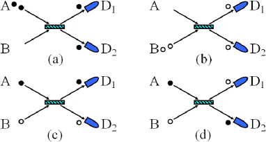
In the view of quantum theory, either the correlation or the anti-correlation of thermal radiation is the result of two-photon interference, which involves the nonlocal superposition of two-photon amplitudes tpith . Analogous to Dirac’s statement that a photon interferes with itself, this interference is a jointly measured pair of independent photons interfering with the pair itself. Figure 5 schematically illustrates four alternatives for two independent photons to trigger a joint-detection event of $D_{1}$ and $D_{2}$. In (a) and (b) the measured pair comes from the same fiber tip, $A$ or $B$. In (c) and (d) the measured pair comes from different fiber tips, one from $A$ and the other from $B$. It is the superposition between amplitudes in (c) and (d) that produces the anti-correlation.

Figure 5: There are four alternative ways for a measured pair of independent photons to trigger a joint-detection event of $D_{1}$ and $D_{2}$.

Now we give a formal quantum mechanical calculation. The probability of observing a joint-detection event at space-time coordinates $(\mathbf{r}_{1},t_{1})$ and $(\mathbf{r}_{2},t_{2})$ is given in Eq. (4), in which the fields $E(\mathbf{r}_{1},t_{1})$ and $E(\mathbf{r}_{2},t_{2})$ are treated as the superposition of the early fields at the input planes $z=d_{A}$ and $z=d_{B}$

$$\hat{E}^{(+)}(z_{1},t_{1}) =\frac{1}{\sqrt{2}}[\hat{E}^{(+)}(\tau_{A1})+\hat{E}^{(+)}(\tau_{B1})]$$

$$\hat{E}^{(+)}(z_{2},t_{2}) =\frac{1}{\sqrt{2}}[\hat{E}^{(+)}(\tau_{A2})-\hat{E}^{(+)}(\tau_{B2})].$$ (7)

where $\tau_{Aj}\equiv t_{j}-r_{Aj}/c$, $j=1,2$, the optical delay from the detector $D_{j}$ to the input plane $A$, $n$ the index of refraction of the fiber, and $\tau_{Bj}$ is defined similarly.

To simplify the calculation, we assume two groups of randomly distributed wavepackets are excited at the fiber tips $A$ and $B$

$$|\Psi_{A}\rangle =\int d\omega\,f(\omega)\,e^{i\omega t_{0A}}\,\hat{a}^{{\dagger}}(\omega)\,|0\rangle$$

$$|\Psi_{B}\rangle =\int d\omega\,f(\omega)\,e^{i\omega t_{0B}}\,\hat{b}^{{\dagger}}(\omega)\,|0\rangle,$$ (8)

where $f(\omega)$ is the spectrum function which is mainly determined by the spectral filters (IF) in the experimental setup, $t_{0A}$ and $t_{0B}$ represent the times when the wavepackets pass the planes $A$ and $B$, respectively.

Substituting the field and the density operators into Eq. (4), it is straightforward to find that

$$\ \ \ \ G^{(2)}(z_{1},t_{1};z_{2},t_{2})$$

$$=|\mathscr{A}(\tau^{T}_{A1},\tau^{R}_{A2})|^{2}+|\mathscr{A}(\tau^{R}_{B1},\tau^{T}_{B2})|^{2}$$

$$\ \ \ +\left|\mathscr{A}(\tau^{T}_{A1},\tau^{T}_{B2})-\mathscr{A}(\tau^{R}_{A2},\tau^{R}_{B1})\right|^{2},$$ (9)

with

$$\mathscr{A}(\tau^{T}_{A1},\tau^{R}_{A2}) =\langle 0|\hat{E}^{(+)}(\tau_{A1})|\Psi_{A}\rangle\langle 0|\hat{E}^{(+)}(\tau_{A2})|\Psi_{A}\rangle$$

$$\mathscr{A}(\tau^{R}_{B1},\tau^{T}_{B2}) =\langle 0|\hat{E}^{(+)}(\tau_{B1})|\Psi_{B}\rangle\langle 0|\hat{E}^{(+)}(\tau_{B2})|\Psi_{B}\rangle$$

$$\mathscr{A}(\tau^{T}_{A1},\tau^{T}_{B2}) =\langle 0|\hat{E}^{(+)}(\tau_{A1})|\Psi_{A}\rangle\langle 0|\hat{E}^{(+)}(\tau_{B2})|\Psi_{B}\rangle$$

$$\mathscr{A}(\tau^{R}_{B1},\tau^{R}_{A2}) =\langle 0|\hat{E}^{(+)}(\tau_{B1})|\Psi_{B}\rangle\langle 0|\hat{E}^{(+)}(\tau_{A2})|\Psi_{A}\rangle,$$

where, $\tau^{T}_{A1}=(t_{1}-t_{0A})-r_{A1}/c$ ($\tau^{R}_{B1}=(t_{1}-t_{0B})-r_{B1}/c$) indicating the early time at points $A$ ($B$) by propagating through the reflected (transmitted) optical path from source $A$ ($B$) to the photo-detector $D_{1}$; and $\tau^{R}_{A2}=(t_{2}-t_{0A})-r_{A2}/c$ ($\tau^{T}_{B2}=(t_{2}-t_{0B})-r_{B2}/c$), indicating the early time at points $A$ ($B$) by propagating through the transmitted (reflected) optical path from $A$ ($B$) to the photo-detector $D_{2}$; $t_{0A}$ and $t_{0B}$ are the initial times at $A$ and $B$, respectively. These four effective wave functions correspond to the four alternatives shown in Fig.5. It is not difficult to see that the first two terms in Eq. (Observation of Anti-correlation of Classical Chaotic Light) are $\delta$ independent. The two-photon interference occurs in the third term. The cross two-photon interference term in the third term gives

$$\mathscr{A}^{*}(\tau^{T}_{A1},\tau^{T}_{B2})\mathscr{A}(\tau^{R}_{B1},\tau^{R}_{A2})\simeq e^{-\delta^{2}/\tau_{c}^{2}}$$

for a Gaussian spectrum function of $f(\omega)$. The details are given in Appendix B. The coincidence coincident counting rate is therefore,

$$R_{c}\simeq R_{0}\int dt_{1}dt_{2}\,G^{(2)}(z_{1},t_{1};z_{2},t_{2})\propto 1-\frac{1}{2}e^{-\delta^{2}/\tau_{c}^{2}}.$$ (10)

Eq. (10) has been verified by achieving different coherence time of the chaotic filed, which are determined by different bandwidth of the spectral filters (IF), as shown in Fig.3 (I) and (II), except with lower contrasts [$\sim 28\%$ for (I) and $\sim 29\%$ for (II)].

In conclusion, we have observed a nonclassical anti-correlation from classical chaotic light under the experimental condition of $G^{(1)}_{AB}=0$. The classical statistical correlation theory seems unable to explain this experimental result. This observation is different from all historical measurement of the “dips”, either observed from nonclassical sources or from synchronized coherent sources. In the view of quantum mechanics, either the anti-correlation “dip” or the correlation “peak” of thermal light are straightforward two-photon interference phenomena, involving the superposition of two-photon amplitudes.

The authors wish to thank T.B. Pittman, M.H. Rubin, J.P. Simon, Y. Zhou, G. Scarcelli and V. Tamma for helpful discussions. This research was partially supported by AFOSR and ARO-MURI program. Z. Xie acknowledges his partial support from China Scholarship Council.

Appendix A Appendix A: Classical Statistical Intensity Correlation

The standard statistics of classical chaotic light gives the second order correlation in Eq. (3). Eq. (3) can be explicitly calculated as

$$\ \ \ \ \Gamma^{(2)}(\mathbf{r}_{1},t_{1};\mathbf{r}_{2},t_{2})=\langle I(\mathbf{r}_{1},t_{1})\,I(\mathbf{r}_{2},t_{2})\rangle$$

$$=\langle\big{|}E(\mathbf{r}_{A},t_{1A})+E(\mathbf{r}_{B},t_{1B})\big{|}^{2}\big{|}E(\mathbf{r}_{A},t_{2A})-E(\mathbf{r}_{B},t_{2B})\big{|}^{2}\rangle$$

$$=\langle\big{|}E(\mathbf{r}_{A},t_{1A})\big{|}^{2}\rangle\,\langle\big{|}E(\mathbf{r}_{A},t_{2A})\big{|}^{2}\rangle$$

$$\ \ \ +\langle E^{*}(\mathbf{r}_{A},t_{1A})E(\mathbf{r}_{A},t_{2A})\rangle\langle E(\mathbf{r}_{A},t_{1A})E^{*}(\mathbf{r}_{A},t_{2A})\rangle$$

$$\ \ \ +\langle\big{|}E(\mathbf{r}_{B},t_{1B})\big{|}^{2}\rangle\,\langle\big{|}E(\mathbf{r}_{B},t_{2B})\big{|}^{2}\rangle$$

$$\ \ \ +\langle E^{*}(\mathbf{r}_{B},t_{1B})E(\mathbf{r}_{B},t_{2B})\rangle\langle E(\mathbf{r}_{B},t_{1B})E^{*}(\mathbf{r}_{B},t_{2B})\rangle$$

$$\ \ \ +\langle\big{|}E(\mathbf{r}_{A},t_{1A})\big{|}^{2}\rangle\,\langle\big{|}E(\mathbf{r}_{B},t_{2B})\big{|}^{2}\rangle$$

$$\ \ \ +\langle\big{|}E(\mathbf{r}_{B},t_{1B})\big{|}^{2}\rangle\,\langle\big{|}E(\mathbf{r}_{A},t_{2A})\big{|}^{2}\rangle$$ (11)

$$\ \ \ -\langle E^{*}(\mathbf{r}_{A},t_{1A})E(\mathbf{r}_{A},t_{2A})\rangle\langle E(\mathbf{r}_{B},t_{1B})E^{*}(\mathbf{r}_{B},t_{2B})\rangle$$

$$\ \ \ -\langle E(\mathbf{r}_{A},t_{1A})E^{*}(\mathbf{r}_{A},t_{2A})\rangle\langle E^{*}(\mathbf{r}_{B},t_{1B})E^{(}\mathbf{r}_{B},t_{2B})\rangle$$

where, again, $(\mathbf{r}_{A},t_{jA}=t_{j}-r_{jA}/c)$ and $(\mathbf{r}_{B},t_{jB}=t_{j}-r_{jB}/c$), $j=1,2$, are the earlier space-time coordinates. Eq. (A) can be written in the following form

$$\Gamma^{(2)}=\Gamma^{(1)}_{A11}\,\Gamma^{(1)}_{A22}+\Gamma^{(1)}_{A12}\,\Gamma^{(1)}_{A21}+\Gamma^{(1)}_{B11}\,\Gamma^{(1)}_{B22}+\Gamma^{(1)}_{B12}\,\Gamma^{(1)}_{B21}$$

$$+\Gamma^{(1)}_{A11}\,\Gamma^{(1)}_{B22}+\Gamma^{(1)}_{A22}\,\Gamma^{(1)}_{B11}-\Gamma^{(1)}_{A12}\,\Gamma^{(1)}_{B21}-\Gamma^{(1)}_{A21}\,\Gamma^{(1)}_{B12}.$$ (12)

Here, all the terms $\Gamma^{(1)}_{AB}\Gamma^{(1)}_{AB}$ vanish due to mutual incoherence nature between the fields $E(\mathbf{r}_{A},t_{A})$ and $E(\mathbf{r}_{B},t_{B})$, leaving the non-zero terms $\Gamma^{(1)}_{AA}\Gamma^{(1)}_{AA}$, $\Gamma^{(1)}_{BB}\,\Gamma^{(1)}_{BB}$ and $\Gamma^{(1)}_{AA}\Gamma^{(1)}_{BB}$ contributing to $\Gamma^{(2)}$. The negative signs in the last two terms are basically introduced by beamsplitter. It is not too difficult to find from Eq. (A) that $\Gamma^{(2)}$ is independent of the optical delay $\delta$ for either CW or pulsed chaotic light.

Case (I): CW chaotic light

There is no doubt the first four terms are $\delta$ independent. In these terms either the self-correlations, $\Gamma^{(1)}_{A11}\Gamma^{(1)}_{A22}$ and $\Gamma^{(1)}_{B11}\Gamma^{(1)}_{B22}$, or the cross-correlations, $\Gamma^{(1)}_{A12}\Gamma^{(1)}_{A21}$ and $\Gamma^{(1)}_{B12}\Gamma^{(1)}_{B21}$ are respectively associated with the same radiation $A$ or $B$. The other four terms may contain $\delta$ in their amplitude part or in their phase part. We do not need to worry about the amplitude part due to the stationary nature of the CW chaotic light. Let us examine the phase part: (1) the first two terms $\Gamma^{(1)}_{A11}\Gamma^{(1)}_{B22}=\langle I_{A11}\rangle\langle I_{B22}\rangle$ and $\Gamma^{(1)}_{A22}\Gamma^{(1)}_{B11}=\langle I_{A22}\rangle\langle I_{B11}\rangle$ contain the expectation of intensities only and thus are phase independent. (2)The second two terms $\Gamma^{(1)}_{A12}\Gamma^{(1)}_{B21}$ and $\Gamma^{(1)}_{A21}\Gamma^{(1)}_{B12}$ may contain relative phases of $k(r_{A1}-r_{A2})$ and $k(r_{B1}-r_{B2})$, however, these phases are $\delta$ independent. We may conclude in the case of CW chaotic light, $\Gamma^{(2)}$ is independent of the optical delay $\delta$.

Case (II): Pulsed chaotic light

All the analysis are the same as above, except we do need to consider the delays between the amplitudes, which is $\delta$ dependent. In the pulsed case, the fields are non-stationary, the last four terms have nonzero values only when their amplitudes have nonzero values simultaneously in the joint-detection of $D_{1}$ and $D_{2}$. It is clear when $\delta=0$, all four terms achieve their maximum values simultaneously due to the complete overlapping of their respective amplitudes. The overall contribution of the four terms, however, is null to $\Gamma^{(2)}$ due to the cancelation between the first two positive contributions and the last two negative contributions. When $\delta$ increase or decrease from zero, although the overlapping between the $A$ amplitude and the $B$ amplitude becomes smaller and smaller yielding smaller contributions to $\Gamma^{(2)}$, the overall contribution keeps its zero vale for the same reason. We may conclude that in the case of pulsed chaotic light, $\Gamma^{(2)}$ is independent of the optical delay $\delta$ too.

Appendix B Appendix B: Quantum Theory

In Appendix B we show a simple calculation of the effective wave functions. The effective-wavefunctions corresponding to the case in which the joint-detection event is produced by two photon coming from the same point is shown below as an example

$$\ \ \ \mathscr{A}(\tau^{T}_{A1},\tau^{R}_{A2})=\langle 0|\hat{E}^{(+)}(\tau_{A1})|\Psi_{A}\rangle\langle 0|\hat{E}^{(+)}(\tau_{A2})|\Psi_{A}\rangle$$

$$\propto\int d\omega f(\omega)e^{-i\omega\tau^{T}_{A1}}\int d\omega^{\prime}f(\omega^{\prime})e^{-i\omega^{\prime}\tau^{R}_{A2}}$$

$$=e^{-i\omega_{0}\tau^{T}_{A1}}\mathcal{F}_{\tau^{T}_{A1}}\{f(\nu)\}e^{-i\omega_{0}\tau^{R}_{A2}}\mathcal{F}_{\tau^{R}_{A2}}\{f(\nu)\}$$ (13)

where,

$$\mathcal{F}_{\tau}\{f(\nu)\}\equiv\int d\nu f(\nu)e^{-i\nu\tau}$$

is the fourier transform of the spectrum function $f(\nu)$, and $\nu=\omega-\omega_{0}$ ($\omega_{0}$ is the central frequency). It is easy to see these functions are $\delta$ independent.

The superposition of the two-photon amplitudes (c) and (d) corresponding to the interference term in Eq. (Observation of Anti-correlation of Classical Chaotic Light) is calculated to be

$$\ \ \ \ \big{|}\mathscr{A}(\tau^{T}_{A1},\tau^{T}_{B2})-\mathscr{A}(\tau^{R}_{B1},\tau^{R}_{A2})\big{|}^{2}$$ (14)

$$=\big{|}\mathcal{F}_{\tau^{T}_{A1}}\big{\{}f(\nu)\big{\}}\mathcal{F}_{\tau^{T}_{B2}}\big{\{}f(\nu)\big{\}}\big{|}^{2}+\big{|}\mathcal{F}_{\tau^{R}_{B1}}\big{\{}f(\nu)\big{\}}\mathcal{F}_{\tau^{R}_{A2}}\big{\{}f(\nu)\big{\}}\big{|}^{2}$$

$$\ \ \ -\mathcal{F}^{*}_{\tau^{T}_{A1}}\big{\{}f(\nu)\big{\}}\mathcal{F}^{*}_{\tau^{T}_{B2}}\big{\{}f(\nu)\big{\}}\mathcal{F}_{\tau^{R}_{B1}}\big{\{}f(\nu)\big{\}}\mathcal{F}_{\tau^{R}_{A2}}\big{\{}f(\nu)\big{\}}$$

$$\ \ \ -\mathcal{F}_{\tau^{R}_{A1}}\big{\{}f(\nu)\big{\}}\mathcal{F}_{\tau^{T}_{B2}}\big{\{}f(\nu)\big{\}}\mathcal{F}^{*}_{\tau^{R}_{B1}}\big{\{}f(\nu)\big{\}}\mathcal{F}^{*}_{\tau^{R}_{A2}}\big{\{}f(\nu)\big{\}}.$$

It is easy to find that the first two terms in Eq. (14) contribute a constant to the coincidence counting rate $R_{c}$. The nontrivial contributions come from the last two cross terms. Assuming a Gaussian spectrum, the cross terms is approximately to be

$$\mathcal{F}^{*}_{\tau^{T}_{A1}}\big{\{}f(\nu)\big{\}}\mathcal{F}^{*}_{\tau^{T}_{B2}}\big{\{}f(\nu)\big{\}}\mathcal{F}_{\tau^{R}_{B1}}\big{\{}f(\nu)\big{\}}\mathcal{F}_{\tau^{R}_{A2}}\big{\{}f(\nu)\big{\}}\propto e^{-\delta^{2}/\tau^{2}_{c}},$$

for synchronized radiations $A$ and $B$, i.e., $t_{0A}=t_{0B}$, where $\tau_{c}$ is the coherence time of the measured field. It is interesting to see the cross term contribution is time independent. The coincidence counting rate is therefore

$$R_{c}\simeq R_{0}\int dt_{1}dt_{2}\,G^{(2)}(z_{1},t_{1};z_{2},t_{2})\propto 1-\frac{1}{2}e^{-\delta^{2}/\tau_{c}^{2}}.$$

References

(1) Hanbury Brown R, and Twiss R Q 1956 Nature177, 27-29; Hanbury Brown R 1974 Intensity
Interferometer (Taylor & Francis, London).
(2)
Scarcelli G, Berardi V, and Shih Y H 2006 Phys. Rev. Lett.96,
063602. Note, the natural, non-factorizable, point-to-point, near-field-image-forming
correlation in the lensless ghost imaging is in principle different from these
classical simulations, such as the man-made, factorizable, “speckle to speckle”,
correlation of A. Gatti et al. [A. Gatti et al, Phys. Rev. A 70,
013802, (2004), and Phys. Rev. Lett. 93, 093602 (2004)]. The original
publications of Gatti et al. choose 2f-2f classical imaging systems,
, to image the “speckles” of the light source onto the object
plane and the ghost image plane, respectively. Their speckle-speckle correlation
is factorizeable into two classical images of “speckles”.
(3) makes
this experiment different from all other demonstrations of
interference between independent light sources. Mandel et al.
showed that radiations from two independent sources can produce
first-order interference for an single-shot exposure, if the
“exposure” time is shorter than the coherence time of the fields.
See, Magyar G, Mandel L 1963 Nature, 198, 255; Mandel
L 1983 Phys. Rev. A, 28, 929. In a time integrated
multi-exposure measurement, the first-order interference pattern may
not be observable due to the phase variation from one exposure to
another exposure. However, the joint-detection of two individual
photodetectors may still produce observable second-order correlation
or anti-correlation. In our experiment, is
chosen to be zero. The classical interpretation of time averaged
effect of classical mutual coherence or partial mutual coherence
does not apply.
(4) Martienssen W and Spiller E 1964 Am. J. Phys.32, 919.
(5) Glauber R J 1963 Phys. Rev.10 84;
Glauber R J 1963 Phys. Rev.130, 2529. In
Eq. (4), we use to distinguish quantum
correlation from classical statistical intensity correlation of
.
(6) Jeltes T, et al. 2007
Nature 445, 402-405.
(7) Hong C K, Ou Z Y and Mandel L 1987 Phys. Rev. Lett.59, 2044;
Shih Y H and Alley C O 1988 Phys. Rev. Lett.61,
2921. In the Alley-Shih two-photon interferometer, both
anti-correlation “dip” and correlation “peak” are observable by
selecting different polarization of the entangled photon pair.
(8) Loudon R 2000 The Quantum Theory of
Light (Oxford, New York, 3rd Edition ).
(9)G. Scarcelli, A. Valencia
and Shih Y H 2004 EuroPhys. Lett.68: 618.