Interplay of Quantum Criticality and Geometric Frustration in Columbite

Abstract

Motivated by CoNb₂O₆ (belonging to the columbite family of minerals), we theoretically study the physics of quantum ferromagnetic Ising chains coupled anti-ferromagnetically on a triangular lattice in the plane perpendicular to the chain direction. We combine exact solutions of the chain physics with perturbative approximations for the transverse couplings. When the triangular lattice has an isosceles distortion (which occurs in the real material), the $T=0$ phase diagram is rich with five different states of matter: ferrimagnetic, Néel, anti-ferromagnetic, paramagnetic and incommensurate phases, separated by quantum phase transitions. Implications of our results to experiments on CoNb₂O₆ are discussed.

Two of the most exciting themes in condensed matter physics are the destruction of magnetic order at absolute zero temperature, i.e. quantum criticality subir , and quantum fluctuations in geometrically frustrated magnets. Each of these themes has its archetype: the quantum Ising chain in a transverse field subir for quantum criticality, and the triangular lattice Ising model for geometrical frustration  Wannier . Remarkably both these ideals are combined in CoNb₂O₆, a material which may be understood as a collection of weakly coupled Ising chains that sit on a triangular lattice in the plane perpendicular to the chain direction. Very recently, CoNb₂O₆ has been the subject of beautiful single crystal inelastic neutron scattering experiments by Coldea et al coldeaXX . The observed spectrum has been shown to reflect some very subtle properties of one-dimensional Ising quantum critical physics, that were discovered three decades after the study of the quantum Ising chain was initiated lsm61 , in a triumph of theoretical physics led by Zamolodchikov zamo89 . A full interpretation of the experimental data requires an understanding of the interplay of quantum criticality in the chain and the physics of frustration in the plane perpendicular to the chain. In this paper, we combine the remarkable insights of Zamolodchikov with the novelty that frustration brings to the phase diagram of this remarkable material, setting up a platform to understand the experimental data in totality. Our focus here is to chart out the global phase diagram of CoNb₂O₆, as well as other less well studied materials that have similar structures.

CoNb₂O₆ is an insulator. A strong single ion anisotropy forces the spin on the magnetically active Co²⁺ (3d⁷) ions to point either “up” or “down” along the local easy axis, realizing a two-level system. The Co²⁺ ions interact with each other through Ising interactions of the form $S^{z}_{i}S^{z}_{j}$, where $\vec{S}_{i}$ are the usual spin-1/2 operators acting on the two level system located at site $i$. A magnetic field applied along the b-axis is transverse to all the easy axes and hence may be modeled by a term, $h_{\perp}S^{x}_{i}$, which acts like a transverse field on the Ising spins. In the absence of the transverse field the exchange interactions will cause the Ising spins to order magnetically. On the other hand when $h_{\perp}$ is much larger than the exchange interactions, the Ising spins will all lie in the quantum superposition, $(|\uparrow\rangle+|\downarrow\rangle)/\sqrt{2}$, highlighting the fact that the transverse field is a quantum mechanical parameter with no classical analogue. The central question of interest that we will address in this publication is: What is the nature of the magnetic ordering and what is the sequence of $T=0$ phases between the two extreme limiting cases as $h_{\perp}$ is tuned?

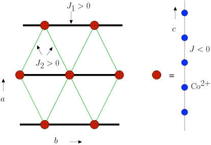
Figure 1: Schematic structure of Co²⁺ ions in CoNb₂O₆. Ising spins localized on each Co²⁺ form ferromagnetic chains running along the c-direction; $J_{0}$ is the strength of the exchange along these c-axis chains. In the basal a-b plane perpendicular to the c-axis, the chains form a triangular lattice. The stronger anti-ferro $J_{1}$ bonds parallel to the b-axis divide the basal triangular lattice into “basal chains” (marked with thick black lines), the weaker anti-ferro $J_{2}=\alpha J_{1}$ bonds (marked with thin green lines) connect neighboring “basal chains”. $1-\alpha\ll 1$ in CoNb₂O₆ is a measure of the departure from a perfect basal triangular lattice in this material.

We begin by presenting a minimal theoretical model for CoNb₂O₆ which incorporates details of the columbite structure and which we expect to reproduce most of the features of the experiments. The lattice consists of zig-zag chains of Co²⁺ ions with a strong ferromagnetic Ising interaction, $J_{0}<0$ along the c-direction. The chains form an isosceles triangular lattice in the a-b plane, with anti-ferromagnetic coupling to neighbors of strength $J_{1}$ and $J_{2}$ as shown in Fig. 1.

$$H=J_{0}\sum S^{z}_{z;{\bf r}}S^{z}_{z+1;{\bf r}}+J_{1}\sum_{{\bf r}}S^{z}_{z;{\bf r}}S^{z}_{z;{\bf r+a_{1}}}+J_{2}\sum_{{\bf r}}S^{z}_{z;{\bf r}}S^{z}_{z;{\bf r+a_{2}}}+J_{2}\sum_{{\bf r}}S^{z}_{z;{\bf r}}S^{z}_{z;{\bf r+a_{3}}}-h_{\perp}\sum S^{x}_{z;{\bf r}},$$ (1)

${\bf a_{1,2,3}}$ are the three nearest neighbors on the triangular lattice illustrated in Fig. 1. Motivated by CoNb₂O₆ we focus on the limit when $0<J_{1},J_{2}\ll|J_{0}|$, the limit of weakly coupled Ising chains. Our focus is on the effects of quantum fluctuations controlled by the transverse field and hence we will not address early experimental work kobayashi ; heid which studied the material in a longitudinal field. Our results with some modifications also apply to other materials which are known to realize Ising spin chains weakly coupled on a triangular lattice cao . Theoretically, a study of the 2-dimensional triangular Ising anti-ferromagnet in a transverse field is available ms , which corresponds to the limit of $J_{0}=0$ of our model. We are interested in the opposite limit in this paper. Were $\alpha\equiv J_{2}/J_{1}=1$, the system would form a perfect triangular lattice in the basal plane. It is known that the material has $\alpha\lesssim 1$ and hence the coupling along the chains running along the x-axis is a little stronger kobayashi . As we shall see, the lattice anisotropy significantly enriches the phase diagram.

When $J_{1},J_{2}=0$ the model Eq. (1) reduces to a collection of one-dimensional Ising chains in a transverse field (TFIC),

$$H_{\rm TFIC}=J_{0}\sum_{i}S^{z}_{i}S^{z}_{i+1}-h_{\perp}\sum_{i}S^{x}_{i}-h_{\parallel}\sum_{i}S^{z}_{i}.$$ (2)

An $h_{\parallel}$ term is included even though we study the model Eq. (1) with no parallel field; the reason for this will become clear below. The TFIC harbors a quantum critical point (between a magnetic and a paramagnetic state when $h_{\parallel}=0$ and $h_{\perp}=J_{0}/2$) in the same universality class as the well studied two-dimensional Ising field theory. Indeed, the singular contribution to the ground state energy of the TFIC Hamiltonian, Eq. (2) can be related to the free energy of the Ising field theory by a simple re-scaling of variables. The scale is set by comparing correlation functions in the TFIC (it can be solved exactly when $h_{\parallel}=0$, see e.g. pfeuty ) to the Ising field theory results fz . We find,

$$E_{\rm TFIC}=\frac{J_{0}}{2}\mathcal{E}_{\rm IFT}\left(\frac{h_{\perp}-J_{0}/2}{J_{0}/2},\frac{c_{h}h_{\parallel}}{J_{0}/2}\right).$$ (3)

We will make use of the scaled variables $\bar{h}_{\perp}=\frac{h_{\perp}-J_{0}/2}{J_{0}/2}$, $\bar{h}_{\parallel}=\frac{c_{h}h_{\parallel}}{J_{0}/2}$ and express all energies in units of $J_{0}/2$ ($c_{h}=\sqrt{\frac{e^{1/4}2^{1/12}}{4A^{3}}}\approx 0.4016$, $A\approx 1.2824$ is Glaisher’s constant). Expansions for the function ${\cal E}_{\rm IFT}(\bar{h}_{\perp},\bar{h}_{\parallel})$ are available fz in different limits for both finite $\bar{h}_{\perp}$ and $\bar{h}_{\parallel}$, when $\xi=\bar{h}_{\parallel}/\bar{h}_{\perp}^{a}\ll 1$ and when the magnitude of $\eta=-\bar{h}_{\perp}/\bar{h}^{1/a}_{\parallel}$ is small,

$${\cal E}^{\bar{h}_{\perp}>0}_{\rm IFT}(\bar{h}_{\perp},\bar{h}_{\parallel}) = \frac{\bar{h}_{\perp}^{2}}{8\pi}\log\bar{h}_{\perp}^{2}+\bar{h}_{\perp}^{2}\left(G_{2}\xi^{2}+G_{4}\xi^{4}+G_{6}\xi^{6}\dots\right),$$

$${\cal E}^{\bar{h}_{\perp}<0}_{\rm IFT}(\bar{h}_{\perp},\bar{h}_{\parallel}) = \frac{\bar{h}_{\perp}^{2}}{8\pi}\log\bar{h}_{\perp}^{2}+\bar{h}_{\perp}^{2}\left(\tilde{G}_{1}|\xi|+\tilde{G}_{2}|\xi|^{2}+\dots\right),$$

$${\cal E}_{\rm IFT}(\bar{h}_{\perp},\bar{h}_{\parallel}) = \frac{\bar{h}_{\perp}^{2}}{8\pi}\log\bar{h}_{\perp}^{2}+\bar{h}_{\parallel}^{16/15}\left[-\frac{\eta^{2}}{8\pi}\log\eta^{2}+\left(\Phi_{0}+\Phi_{1}\eta+\Phi_{2}\eta^{2}+\dots\right)\right],$$ (4)

where $a=15/8$ is a critical index of the Ising universality class. The numbers $G_{n}$, $\tilde{G}_{n}$ and $\Phi_{n}$ are universal numbers which are known to great accuracy, a few are reproduced in Table 1.

In order to expand around the non-trivial TFIC limit we construct a variational wave-function, $|\Psi\rangle=\prod_{i}|\bar{h}_{i}\rangle$, as a product of TFIC ground states, where the longitudinal field $\bar{h}_{\parallel}=\bar{h}_{i}$ defining the TFIC Hamiltonian for each chain is taken as a variational parameters. The variational energy for our model is given by,

$$E_{\rm mf} = \sum_{i}\mathcal{E}_{\rm IFT}(\bar{h}_{\perp},\bar{h}_{i})+\bar{h}_{i}\bar{m}_{i}+\sum\bar{m}_{i}\frac{\bar{J}_{ij}}{2}\bar{m}_{j},$$ (5)

where the magnetization on the $i^{\rm th}$ chain, $\bar{m}_{i}=-\partial\mathcal{E}_{\rm IFT}/\partial\bar{h}_{i}$. Optimization over $\bar{h}_{i}$, gives $\bar{h}_{i}=-\bar{J}_{ij}\bar{m}_{j}$

$$E_{\rm mf} = \sum_{i}\mathcal{E}_{\rm IFT}(\bar{h}_{\perp},\bar{h}_{i})-\sum\bar{h}_{i}\frac{\bar{J}_{ij}^{-1}}{2}\bar{h}_{j}.$$ (6)

Here the labels $i,j$ span sites in a plane (or corresponding chains), and $J_{ij}$ is the interaction between a pair of spins. In addition we have defined the rescaled matrix $\bar{J}_{ij}\equiv c_{h}^{2}J_{ij}/(J_{0}/2)$, whose non-zero entries are $\bar{J}_{1,2}=c_{h}^{2}J_{1,2}/(J_{0}/2)$. Sometimes we prefer to work with the mean-field magnetization, $\bar{m}_{i}=\bar{J}^{-1}_{ij}\bar{h}_{j}$, in which case $E_{\rm mf}=\sum_{i}\mathcal{E}_{\rm IFT}(\bar{h}_{\perp},-\bar{J}_{ij}\bar{m}_{j})-\sum\bar{m}_{i}\frac{\bar{J}_{ij}}{2}\bar{m}_{j}$. The philosophy of our approach is similar to “chain mean-field” theories that has been applied to a number of unfrustrated problems schulz ; tsvelik ; scalapino .

We now study the quantum phase diagram (phases and phase transitions) that arise by extremizing the variational energy Eq. (5) using the exact expansions Eq. (Interplay of Quantum Criticality and Geometric Frustration in Columbite) for the TFIC. We present our results for the phase diagram as a functions of $\bar{J}_{1}$ and $\bar{h}_{\perp}$, for a fixed $\alpha$.

Perfect Triangles: When $\bar{J}_{2}=\bar{J}_{1}$ (i.e. $\alpha=1$), we have perfect equilateral triangles in the basal plane. Treating this coupling in perturbation theory, we approach the magnetic ordering from each of the two phases of the Ising chain, the paramagnetic phase for $\bar{h}_{\perp}>0$ and the magnetic phase for $\bar{h}_{\perp}<0$.

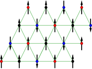
(a) Ferri-magnetic (FR)

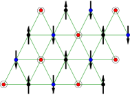
(b) Anti-Ferromagnet (AF)

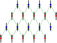
(c) Néel 1 (N1)

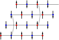
(d) Néel 2 (N2)

Figure 2: Magnetic ordering patterns of FR, AF, N1 and N2 phases. (a) Dividing the lattice into A, B and C sub-lattices (marked red, blue and black), the FR phase corresponds to putting the spins on two of these parallel and the spins on the third anti-parallel, leading to a six-fold degeneracy. (b) The AF state is also a three sub-lattice state but with the spin $\langle S_{i}^{z}\rangle$ on one site fluctuating to zero (c) the two-fold degenerate N1 phase, obtained when $\alpha>1$, can be thought of most simply as the bi-partite (red and blue) Néel phase obtained when the $J_{1}$ bonds are set to zero. (d) the four-fold degenerate N2 phase obtained when $\alpha<1$ corresponds to a Néel ordering along the basal chains ($J_{1}$ bonds) and a ferromagnetic locking of alternate chains (shown by dashed lines).

When $\bar{h}_{\perp}<0$, each isolated chain has a two-fold degenerate magnetic state. Once the chains are coupled this degeneracy is lifted by the exchange fields from the neighbors. Working perturbatively, we expand the energy Eq. (6) order by order in $\bar{J}_{1}$ till the degeneracy is fully lifted. At leading order after minimizing the energy with respect to the magnitude of $\bar{m}_{i}$, $E_{\rm mf}\approx\bar{m}_{i}\frac{\bar{J}_{ij}}{2}\bar{m}_{j}$, (with $|\bar{m}_{i}|$ fixed) i.e. we obtain the classical triangluar lattice Ising model for the signs of $\bar{m}_{i}$. It is well known that there is an extensive degeneracy of configurations which minimize the energyWannier , i.e. ground states consist of all configurations with exactly one pair of parallel spins ($\bar{m}_{i}$ of the same sign) on each elementary triangle. We must continue expanding in $\bar{J}_{1}$ to find how this entropy is finally lifted. At next order, the free energy receives a contribution, $\delta E_{\rm mf}\approx\tilde{G}_{2}\sum_{i}|\bar{h}_{\perp}|^{2-2a}(\bar{J}_{ij}m_{j})^{2}$. Since $\tilde{G}_{2}<0$, this perturbation prefers to have spins on all elementary hexagons parallel. So finding the quantum ground state of our model when $\bar{h}_{\perp}<0$ is reduced to finding the classical ground state of the model, $H=J\sum_{\langle ij\rangle}\sigma_{i}\sigma_{j}-K\sum_{i}\left(\sum_{a}\sigma_{i+e_{a}}\right)^{2}$ where $e_{a}$ are all the neighbors of a site, when $K,J>0,K\ll J$ and $\sigma_{i}=\pm 1$. We find that the ground state (proven in  I.1) is a three-sublattice ferrimagnetic state with spins pointing up on the $A$ sub-lattice and the spins pointing down on the B and C sub-lattices (there are a total of 6 symmetry-related states). We denote this state as FR, see Fig. 2.

When $\bar{h}_{\perp}>0$, the isolated chains are in a non-degenerate gapped paramagnetic (PM) state. Perturbation theory in the coupling $\bar{J}_{1}$ leaves this state stable and hence there is always a region of PM for small enough $\bar{J}_{1}$. We can now ask if we increase $\bar{J}_{1}$ what magnetic order will first condense. The primary condensation takes place at $(4\pi/3,0)$. Since the order parameters are small, in this regime we can perform a Landau expansion for the order parameter. We have to consider both the complex order parameter at ${\bf Q_{c}}=(4\pi/3,0)$ which we call $\Phi$ and the real uniform component at $(0,0)$ which we call $m$: $h_{i}=\Phi e^{\bf iQ_{c}\cdot r}+\Phi^{*}e^{\bf-iQ_{c}\cdot r}+m$. Keeping only the terms relevant to our study from the most general expansion for these two fields, we arrive at the following Landau continuum expression for the energy density $E_{\rm mf}\approx\int d^{2}r\epsilon_{\rm L}$, ignoring gradient terms,

$$\epsilon_{\rm L}=\alpha_{\Phi}|\Phi|^{2}+\beta_{\Phi}|\Phi|^{4}+\alpha_{m}m^{2}+\lambda_{3}m(\Phi^{3}+\Phi^{*3})+\lambda_{6}(\Phi^{6}+\Phi^{*6})$$ (7)

The coeffecients are fixed by the parameters, $G_{2},G_{4},G_{6},\bar{h}_{\perp}$ and $\bar{J}$. As $\bar{J}_{1}$ is increased, the condensation of $\Phi$ takes place when $\alpha_{\Phi}=0$ (note however $\alpha_{m}$ remains non-zero) in Eq. (7), when $\bar{J}^{c}_{1}=\frac{1}{6|G_{2}|}\bar{h}_{\perp}^{2a-2}$. We can then optimize $m$ for a given configuration of $\Phi$, $m=-\lambda_{3}/(2\alpha_{m})(\Phi^{3}+\Phi^{*3})$ and eliminate it from the energy. This shifts the $\lambda_{6}$ term to $\lambda_{6}-\lambda_{3}^{2}/(4\alpha_{m})$, which evaluates to $\frac{3G_{2}G_{6}-8G_{4}^{2}}{3G_{2}}\bar{h}_{\perp}^{2-6a}>0$ at the critical point. This favors states in which $\Phi^{6}$ is real and negative, so that the phase $\theta$ defined by $\Phi=|\Phi|e^{i\theta}$ is pinned to $\pi/2$. Magnetic order with $\Phi=|\Phi|e^{i\pi/2}$ and $m=0$ corresponds to an anti-ferromagnetic state, we call ${\bf AF}$, illustrated in Fig. 2 (b). This establishes that the ${\bf AF}$ order forms first when the critical $\bar{J}^{c}_{1}$ is crossed.

The pattern of magnetic ordering close to $\bar{h}_{\perp}=0$ can be found using the $\eta$-expansion. In this regime, we find with $\eta=0$ that the FR state has the lowest energy and this state can be smoothly connected to the state found for $\bar{h}_{\perp}<0$.

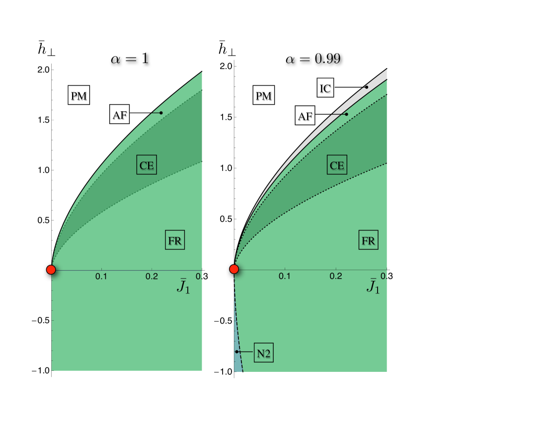
Figure 3: Calculated phase diagram for model, Eq. (1) for perfect triangles, $\alpha\equiv J_{2}/J_{1}=1$, (left) and with an isosceles distortion $\alpha=0.99$ (right). The red dot indicates the Ising quantum critical point of the decoupled chains. The region marked CE is a co-existense between the AF and FR states. It was estimated by using a numerical interpolation for the different expansions of the scaling form of the energy.

Putting together the results from the three expansions, when $\bar{h}_{\perp}>0$, $\bar{h}_{\perp}<0$ and $\bar{h}_{\perp}=0$, we find that the simplest form of the phase diagram consistent with these expansions is the one shown in Fig. 3(a). On general grounds, the transition between ${\bf FR}$ and ${\bf AF}$ can either be direct and and first-order, or it may proceed through a region of “coexistence” corresponding to states with complex $\Phi^{6}$.

Isosceles Triangles: Now we adapt and extend the above analysis to the more complicated case when $\alpha=\bar{J}_{2}/\bar{J}_{1}\neq 1$, resulting from an isosceles distortion of the triangular lattice in the basal plane (as occurs in the real material).

When $\bar{h}_{\perp}<0$, once again there is a macroscopic degeneracy associated with the spontaneous symmetry breaking on each chain which will be lifted by the $\bar{J}_{1,2}$ interactions. Exactly as in the $\alpha=1$ case, at leading order, we have an Ising model for $m_{i}$, but now on an anisotropic lattice, $E_{\rm mf}=\bar{m}_{i}\frac{\bar{J}_{ij}}{2}\bar{m}_{j}$. For $\alpha>1$ the ground state is a two-fold degenerate Néel state (N1), shown in Fig. 2. For $\alpha<1$ (the case in CoNb₂O₆), the situation is more complicated, and at leading order the ground state still has a degeneracy. The triangular lattice in the basal plane can be divided into “basal” chains (not to be confused with the c-axis Ising chains), see Fig. 1, each of which is Néel ordered, however each basal chain can be shifted by a unit without lifting the degeneracy. In fact, in mean field theory this sub-extensive degeneracy is not lifted at all, an artifact of this approximation. Instead, a full perturbative expansion splits the degeneracy at fourth order (see Appendix I.2), by creating a ferro-magnetic interaction between alternate basal Néel chains (even and odd basal chains get locked separately). This effective interaction is a quantum fluctuation effect, not present in the classical $h_{\perp}=0$ limit. The phase shift between even and odd basal chains is determined spontaneously and leads to an extra 2-fold degeneracy, resulting in a 4-fold degeneracy for the N2 state. For a fixed $\bar{h}_{\perp}<0$ and $1-\alpha\ll 1$, for arbitrarily small $\bar{J}_{1}$, we have shown that the N2 state is selected. If $\bar{J}_{1}$ is made large enough however one expects a transition back into the FR state. The phase boundary between N2 and FR is first order, and can be estimated by asking how big $\bar{J}_{1}$ should be so that the $\delta E_{\rm mf}\approx\tilde{G}_{2}\sum_{i}|\bar{h}_{\perp}|^{2-2a}(\bar{J}_{ij}m_{j})^{2}$ (derived above for $\alpha=1$) term that picks the FR state is large enough to close the gap that the anisotropy opens; we find $\bar{J}_{1}^{\rm N2-FR}=\frac{\bar{h}_{\perp}^{2a-2}(1-\alpha)}{2|\tilde{G}_{2}|((1+2\alpha)^{2}-3)}$.

When $\bar{h}_{\perp}>0$, we proceed as in the case of perfect triangles. For small $\bar{J}_{1}$ the PM state is stable. However, at sufficiently strong coupling there is again a condensate but it occurs at an incommensurate wave-vector. The onset wave-vector is determined completely by $\alpha$, it is $(q_{x}^{*},0)$, where $q_{x}^{*}=2\cos^{-1}\left(-\frac{\alpha}{2}\right)$, shifted from $(4\pi/3,0)$. The phase transition will occur again when the coefficient of the quadratic term of the $(q_{x}^{*},0)$ boson mode changes sign, this determines the critical coupling: $\bar{J}^{c}_{1}=\frac{\bar{h}_{\perp}^{2a-2}}{2|G_{2}|(2+\alpha^{2})}$. We call this phase with incommensurate magnetic ordering ${\bf IC}$. As $\bar{J}_{1}$ is made even stronger the system will eventually prefer to lock-in to a commensurate ordering vector. For $1-\alpha\ll 1$, this state will be the AF state discussed above. To understand the commensurate-incommensurate phase transition, it is convenient to begin in the commensurate ${\bf Q_{c}}=(4\pi/3,0)$ AF phase. We can then understand the transition to the incommensurate state as the formation of a dilute condensate of domain walls (which separate the 6 degenerate minima). We begin by evaluating the mean-field energy, for configurations of the form $\bar{h}_{i}=|\Phi|\left[e^{i({\bf Q_{c}\cdot r_{i}}+\theta({\bf r_{i}}))}+{\rm c.c.}\right]+m$, where $\theta({\bf r})$ is a smooth field which creates a domain wall when it shifts between domains, $\theta=(2\pi/6)n$. Owing to the anisotropy of the problem, we may assume that (apart from fluctuations), $\theta({\bf r})$ depends only upon $x$. After coarse-graining and extremizing with respect to $m$, we then obtain the famous sine-Gordon model chaikin ,

$$E_{\rm sg}=A_{yz}\int dx\left[\frac{\kappa}{2}(\partial_{x}\theta)^{2}+\delta_{x}\partial_{x}\theta+\lambda\cos(n_{\rm sg}\theta)\right],$$ (8)

where $A_{yz}$ is the sample area in the $y-z$ plane, and the couplings of the SG model can be related to the parameters in Eq. (6) as worked out explicitly in Appendix I.3; $n_{\rm sg}=6$. From these expressions, we can calculate the phase boundary between the commensurate AF state and the IC state at leading order in $(1-\alpha)$: $\bar{J}^{\rm CIT}_{1}=\bar{J}^{c}_{1}+\mathcal{A}_{\rm CIT}\bar{h}_{\perp}^{2a-2}(1-\alpha)$, where $\mathcal{A}_{\rm CIT}=\frac{G_{4}\pi}{-2G_{2}\sqrt{16G_{4}^{2}-6G_{2}G_{6}}}$ is a pure number.

Our arguments above have predicted a phase diagram shown in Fig. 3 when $1-\alpha\ll 1$. As expected from scaling arguments, all the phase boundaries scale as $\bar{J}\approx\mathcal{A}h^{2a-2}_{\perp}$ when the TFIC’s are close to their individual critical points, where $\mathcal{A}$ is an amplitude which depends on the transition being considered. We have succeeded in computing the amplitudes, $\mathcal{A}$ in some rather non-trivial approximations which we have detailed in the body of the work. Since $\alpha\lesssim 1$ in CoNb₂O₆, our results should apply to this material. Let us now turn to a discussion of the experimental response of each the phases as $\bar{h}_{\perp}$ is increased from zero and to the nature of the phase transitions between them.

Néel phase: This is the phase N2 (illustrated in Fig. 2) which appears with weak external fields. It has no net magnetization and exhibits an elastic neutron peak at momentum $(\tfrac{\pi}{2},0)$ ($(0,\tfrac{1}{2},0)$ in the orthorhombic co-ordinate system). This is in agreement with zero field experimentskobayashi ; heid , though further-neighbor interactions not present in our model could play a role at $h_{\perp}=0$.

Ferri-magnetic phase: As $\bar{h}_{\perp}$ is increased, we expect a first order phase transition into the FR state. The transition N2-FR is driven by the increase of quantum fluctuations of the Ising spins. The FR phase has a net uniform magnetic moment and thus is characterized by elastic neutron peaks both at zero momentum and at the commensurate ordering vector $(4\pi/3,0)$. As $\bar{h}_{\perp}$ is increased we expect the FR order to weaken causing a reduction of the Bragg peaks; the uniform magnetization $m$ and hence zero momentum peak goes to zero as $\bar{h}_{\perp}$ is increased much faster (like the third power) than the peak at $(4\pi/3,0)$.

Anti-Ferromagnetic phase: The AF state also orders at $(4\pi/3,0)$, but it has no uniform component of the magnetization in the z-direction and is hence analogous to an anti-ferromagnet. It is entirely different from the N2 state however, and is truly a result of the geometric frustration present. The difference between the ${\bf AF}$ and ${\bf FR}$ states could be probed by tilting the field in the $b-c$ plane – one expects a weak first order transition at zero tilt in the ${\bf FR}$ case but not the ${\bf AF}$ one.

Incommensurate: As $\bar{h}_{\perp}$ is increased further still, there is a transition into the IC phase that is driven by a condensation of domain walls in the AF phase. The IC phase is characterized by a dense set of Bragg peaks and a massless goldstone (phason) mode. The primary ordering vector, $q_{x}$, shifts continuously in this phase from $q_{x}=4\pi/3$ in the AF phase to value $q_{x}^{*}=2{\rm cos}^{-1}(-\alpha/2)$ at the transition to the PM, the evolution of $q_{x}(\bar{h}_{\perp})$ is described in  I.4).

Paramagnetic: Finally when the quantum fluctuations due to $\bar{h}_{\perp}$ are strong enough, magnetic ordering is completely suppressed and the system enters a quantum paramagnetic phase. This state is gapped and breaks no symmetries of the model, Eq. (1).

Quantum Phase Transitions: There are four quantum phase transitions that we have predicted in the evolution of phases as $\bar{h}_{\perp}$ is tuned. Although the location of these transitions relies on mean field theory, their critical properties are universal. The first transition between N2-FR is expected to be strongly first-order. The second transition is between the FR-AF states. It can take place either by a direct first order transition or through a coexistence of the two phases. Within mean field theory, we find the latter, though this conclusion may be sensitive to the approximation, and to small perturbations of the Hamiltonian. The third transition between the AF-IC state is continuous and is of the commensurate-incommensurate type. We have calculated the leading singularity of the ordering vector here. The final and fourth transition is between IC-PM, which we expect to be in the XY universality class in 4 classical dimensions. Since this is at the upper critical dimension we expect mean field exponents with log corrections. The transverse magnetization as a function of the external field, $h_{\perp}$, should provide a good method for locating the phase transitions. The magnetization itself should have discontinuities at the first order transitions and it’s first derivative should have singularities at the locations of the second order transition.

In summary, we have studied the model, Eq. (1), for CoNb₂O₆ in an external magnetic field that is aligned along the crystallographic b-axis, which results in a fully quantum mechanical “transverse field”. Application of the transverse field drives the frustrated Ising model under study into a number of fascinating phases through quantum phase transitions. We have outlined the basic properties of each of these phases here. Detailed calculations of the excitation spectrum, measurable by neutron scattering, are also possible, and will be presented in a follow-up publication. An interesting question we leave for future exploration is the nature of the finite-temperature phase diagram of this model.

Acknowledgements.- We thank Radu Coldea for stimulating discussions and acknowledge support from the Packard Foundation and National Science Foundation through grants DMR-0804564 and PHY05-51164.

I Supplementary Materials

I.1 Ground state for $\alpha=1$ and $\bar{h}_{\perp}<0$

Here we prove that the ground state of the model on the perfect triangular lattice, $H=\bar{J}\sum_{\langle ij\rangle}\sigma_{i}\sigma_{j}-K\sum_{i}\left(\sum_{a}\sigma_{i+e_{a}}\right)^{2}$, for $\bar{J},K>0$ and $K/\bar{J}\ll 1$ is the FR state. The proof is as follows: We need to find which Ising configuration has the lowest energy with the $K$ term. Lets imagine an Ising configuration on an infinite lattice with $f_{6},f_{5},f_{4},f_{3}$ the fraction of sites that have $6,5,4,3$ anti-parallel neighbors. Then $f_{6}+f_{5}+f_{4}+f_{3}=1$. Also a third of the bonds have to be frustrated (host parallel spins) in any Ising configuration which implies, $f_{5}+2f_{4}+3f_{3}=2$. The contribution of the $K$ term to the energy in this language is: $E=-K(36f_{6}+16f_{5}+4f_{4})$. Since we have two extra equations, and four unknowns, we can rewrite the equation for $E$ completely in terms of $f_{3}$ and $f_{6}$, obtaining $E=-K(4+8(f_{3}+f_{6}))$. Since $f_{3}+f_{6}<1$, the lowest energy is clearly obtained only with $3,6$ sites. This configuration has $f_{6}=1/3$ and $f_{3}=2/3$. The only such configuration is the ferri-magnetic state described above.

I.2 Ground state for $\alpha<1$ and $\bar{h}_{\perp}<0$

In the section we show that the ground state when $\alpha<1$ and when the chains are magnetically ordered is the N2 state for arbitrarily small inter-chain coupling. The goal here is to develop a systematic perturbative expansion about the limit of decoupled Ising chains. On the magnetic side there is a huge degeneracy in this limit because each chain can have its magnetization $m_{i}$ point up or down. Working in imaginary time, we can set it up as follows,

$$\frac{Z}{Z_{0}}=\frac{\int e^{-S_{\rm 1d}-S_{\rm c}}}{\int e^{-S_{\rm 1d}}}=\langle e^{-S_{\rm c}}\rangle,$$ (9)

where $S_{c}=\int d\tau S^{z}_{i}(\tau)\frac{\bar{J}_{ij}}{2}S^{z}_{j}(\tau)$ and all averages are taken over the decoupled limit. Note that in the zero temperature limit, the partition function is simply given by, $Z=e^{-\beta E_{\rm gs}}$. We can calculate the average perturbatively using the cumulant expansion,

$$\langle e^{-S_{\rm c}}\rangle=e^{-\left[\langle S_{\rm c}\rangle-\frac{1}{2!}\langle S^{2}_{\rm c}\rangle_{\rm con}+\frac{1}{3!}\langle S^{3}_{\rm c}\rangle_{\rm con}-\frac{1}{4!}\langle S^{4}_{\rm c}\rangle_{\rm con}+\dots\right]},$$ (10)

where the subscript “con” indicates that we should only keep connected averages. When we have to evaluate the connected averages we can factor the average into products of averages each of which acts within a single chain, since the chains are decoupled at $0^{\rm th}$ order. For an odd number of spins, these single chain averages will be replaced by, e.g. $\langle S^{z}_{i}(\tau)\rangle\rightarrow\bar{m}_{i}|\langle S^{z}(\tau)\rangle|$ with $\bar{m}_{i}=\pm 1$. Then we can ask which configuration of $\bar{m}_{i}$ produces the lowest energy and keep evaluating higher order contributions till any “accidental” degeneracy is completely lifted. The coeffecients of the interactions between $\bar{m}_{i}$ are determined by integrals over correlation functions of the d=1 Ising chain.

We now turn to an evaluation of this approach for the case of interest, when $\alpha<1$. At leading order, we have the term $\bar{m}_{i}\frac{\bar{J}_{ij}}{2}\bar{m}_{j}$, which gives Néel configurations along the stronger bonds that form a chain in the basal plane (not to be confused with the Ising chains in the transverse direction!), but each basal chain can be translated by a unit leading to a $2^{N_{\rm chain}}$ degeneracy (sub-extensive entropy). We expect that the degeneracy is lifted by locking-in of spins on alternate basal chains, but we still need to determine whether the locking-in is ferromagentic or anti-ferromagnetic. At second order, we generate ferro two-spin interactions between alternate basal chains $\propto-\bar{J}_{ij}\bar{J}_{ik}\bar{m}_{j}m^{k}$ but it is easy to see that these cancel when summed over the sites of the basal chain due to the Néel order, i.e., the mean field from all the sites in a chain add up to zero. The degeneracy is not lifted at this order. At third order, we generate both two-spin and four-spin couplings. It turns out that both the two- and four-spin couplings cancel out. At fourth order, we have a large number of generated two-spin couplings and four-spin couplings. Turns out that the four-spin coupling does not lift the degeneracy, but a careful summation of the 86 two-spin couplings does! The two-spin interactions at fourth order are ferromagnetic and hence alternate chains are locked ferromagnetically as shown in Fig. 2.

I.3 Commensurate-Incommensurate Transition

In this section we calculate the energy of a domain wall in the commensurate order parameter as a function of the external parameters. The simplest commensurate-incommensurate transition (CIT) occurs when single domain walls condense chaikin , i.e. when the energy of a single domain wall goes to zero. We can estimate this by a calculation of the domain wall energy. A domain wall corresponds to a spatial profile of the phase $\theta({\bf r})$ of the complex order parameter $\Phi$ introduced earlier in the context of Eq. (7). We hence consider the following form for the field $\bar{h}_{i}$ at site $\bf{r}_{i}$,

$$\bar{h}_{i}=|\Phi|\left[e^{i({\bf Q_{c}}\cdot{\bf r}_{i}+\theta({\bf r}_{i}))}+{\rm c.c.}\right]+m.$$ (11)

Here, ${\bf Q}_{c}$ is a commensurate wave vector $(4\pi/3,0)$ and $\theta({\bf r})$ is a slowly varying functions of r. We substitute this expression into our variational energy, Eq. (5) and then derive a coarse grained energy density for the field $\theta({\bf r})$. Next we integrate out $m$, like we discussed below Eq. (7), arriving at the Sine-Gordon long-wavelength energy for $\theta$, Eq. (8), where we have:

$$\lambda_{6} = \frac{-8G^{2}_{4}+G_{2}G_{6}}{G_{2}}\bar{h}_{\perp}^{2-6a},$$

$$\lambda_{3} = -8G_{4}\bar{h}_{\perp}^{2-4a},$$

$$\alpha_{\rm m} = -3G_{2}\bar{h}_{\perp}^{2-2a},$$

$$\lambda = 2|\Phi|^{6}\left(\lambda_{6}-\frac{\lambda_{3}^{2}}{4\alpha_{\rm m}}\right),$$

$$\kappa_{x} = -|\Phi|^{2}G_{2}\bar{h}_{\perp}^{2-4a},$$

$$\delta_{x} = -|\Phi|^{2}\frac{2G_{2}(1-\alpha)}{\sqrt{3}}h_{\perp}^{2-2a}.$$

Except for $\delta_{x}$, we evaluated all these couplings with $\alpha=1$.

Now we are all set to calculate the transition from the state with commensurate $(4\pi/3,0)$ ordering to the incommensurate phase. Since the $\delta$ term has only an $x$ gradient, we will look for solutions that are translationally invariant in the $y-$direction, dropping all derivatives in this direction. Noting that $\delta$ only gives a boundary term, it may expressed simply as the winding number $N_{w}=[\theta(x=L)-\theta(x=0)]\frac{1}{2\pi/6}$, the number of times the field $\theta$ moves from one its six minima to an adjacent one. The solution for $N_{w}=\pm 1$ is well known,

$$\theta(x)=\frac{4}{n}\tan^{-1}(e^{\pm n_{\rm sg}\sqrt{\frac{\lambda}{\kappa_{x}}}(x-x_{0})}),$$ (12)

where $n_{\rm sg}=6$ in our case.

The energy of a single domain wall is positive for $|\delta|<|\delta_{c}|=4\sqrt{\kappa_{x}\lambda}/\pi$, and the wave vector is commensurate. For $|\delta|>|\delta_{c}|$, domain walls condense and the wave vector is incommensurate. In order to compute the phase boundary, we need the magnetization for a given $\bar{h}_{\perp}$ and $\bar{J}_{1}$ close to the transition when $\alpha=1$. Within our chain-MFT we can compute this by optimizing the mean-field energy. We find,

$$|\Phi|^{2}_{\alpha=1}=\frac{h^{4a-2}_{\perp}}{36G_{4}}\frac{\bar{J}_{1}-\bar{J}^{c}_{1}}{\bar{J}_{1}\bar{J}^{c}_{1}}$$ (13)

where $\bar{J}_{1}^{c}=h^{2a-2}_{\perp}/(6|G_{2}|)$. Now using this as input we can calculate for $1-\alpha\ll 1$ the commensurate-incommensurate phase boundary. We find at leading order in $(1-\alpha)$:

$$\bar{J}^{\rm CIT}_{1}=\bar{J}^{c}_{1}+\mathcal{A}_{\rm CIT}\bar{h}_{\perp}^{2a-2}(1-\alpha)$$ (14)

where $\mathcal{A}_{\rm CIT}=\frac{G_{4}\pi}{-2G_{2}\sqrt{16G_{4}^{2}-6G_{2}G_{6}}}$ is a pure number.

I.4 Ordering vector in the IC

Once the $\bar{h}_{i}$ condense, initially at some incommensurate vector $q_{x}^{*}$, it is clear that the ordering vector will change continuously in the IC phase as $\bar{h}_{\perp}$ is tuned. We can calculate the evolution of the ordering vector from $q_{x}^{*}$ by performing a harmonic expansion valid close to the transition. Approaching the IC phase at high $\bar{h}_{\perp}$ from the PM state, we look for mean-field solutions including a higher harmonic, $\bar{h}_{i}=\Phi_{k}e^{ik\cdot r_{i}}+\Phi_{3k}e^{i3k\cdot r_{i}}+{\rm c.c.}$, which minimize the energy, Eq. (5). We can write the energy density as, $e=\alpha_{k}|\Phi_{k}|^{2}+u_{k}|\Phi_{k}|^{4}+\alpha_{3k}|\Phi_{3k}|^{2}+\lambda_{k}(\Phi^{3}_{k}\Phi^{*}_{3k}+{\rm c.c.})$. Optimizing over $\Phi_{k}$ and $\Phi_{3k}$, we find that minimum energy density is $e=-\frac{\alpha_{k}^{2}}{4u_{k}}-\frac{\lambda_{k}^{2}}{\alpha_{3k}}\left(\frac{-\alpha_{k}}{2u_{k}}\right)^{3}$. If $\lambda_{k}=0$ then the optimal $k=q_{x}^{*}$, but in practice there is a shift, that to leading order in $(1-\alpha)$ and $\bar{h}_{\perp}-\bar{h}_{\perp}^{c}$ is given as,

$$\delta q_{x}=\frac{32(2a-2)^{2}}{9\sqrt{3}}(1-\alpha)\left(\frac{\bar{h}_{\perp}-\bar{h}_{\perp}^{c}}{\bar{h}_{\perp}^{c}}\right)^{2}$$ (15)

from which we conclude that the shift is positive for $(1-\alpha)\ll 1$.

We now turn to the opposite edge of the IC phase, when it borders a commensurate phase, i.e. the AF phase where the ordering takes place at $(4\pi/3,0)$. Once we cross into the IC phase the finite density of domain walls shifts the ordering vector. The shift is given by $\delta q_{x}=2\pi n_{d}$, where $n_{d}$ is the linear density of domain walls. In order to estimate $n_{d}$, we write an expression for the energy of a lattice of domain walls including an interaction energy between domain wall pairs from the SG model (assuming $n_{d}w\ll 1$),

$$\frac{E_{\rm sg}(n_{d})}{A_{yz}}\approx\left(\frac{8\sqrt{\kappa\lambda}}{n_{\rm sg}}-\frac{2\pi\delta_{x}}{n_{\rm sg}}\right)n_{d}+Un_{d}e^{-\frac{1}{wn_{d}}},$$ (16)

where $U>0$ is the strength of repulsion between domain walls and $w=\frac{1}{n_{\rm sg}}\sqrt{\frac{\kappa}{\lambda}}$ is the width of domain walls and controls the range over which they interact. When $\delta_{x}>\delta_{c}=4\sqrt{\kappa\lambda}/\pi$, there is a finite density of domain walls, $n^{*}_{d}\sim\frac{1}{w{\rm ln}|\delta_{c}-\delta_{x}|}$. From this we can estimate the leading singularity in the shift in the ordering vector close to the CIT,

$$\delta q_{x}=\frac{-2\pi}{w\log[\bar{h}_{\perp}-\bar{h}^{\rm CIT}_{\perp}]}$$ (17)

where $w$ is the width of the domain wall at the CIT. From our derived expressions Eq. (I.3) for the coupling constants in the SG model, we can calculate the leading dependence of the domain wall width at the CIT, we find, $w=\frac{2\sqrt{3}}{\pi(1-\alpha)n_{\rm sg}}$. A plot of the two asymptotes for the ordering vector is shown in Fig. 4.

	$n=1$	$n=2$	$n=3$
$G_{2n}$	$-1.84522$	$8.33370$	$-95.1689$
$\tilde{G}_{n}$	$-1.35783$	$-0.0489532$	$0.0387529$
$\tilde{\Phi}_{n-1}$	$-1.19773$	$-0.318819$	$0.1108915$

Table 1: Leading coefficients of the energy expansion of the Ising field theory, appearing in Eq. (Interplay of Quantum Criticality and Geometric Frustration in Columbite), following Ref. fz, .

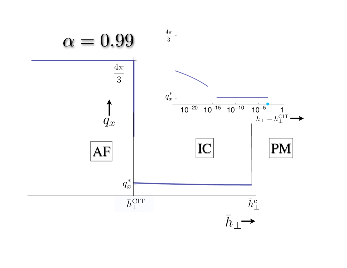
Figure 4: Primary ordering vector in the IC phase. We have computed (in Section I.4) the asymptotics expanding around the CIT and the transition from the PM phase. The evolution of the $q_{x}$ is very sharp as shown. The inset shows the same data on a linear-log plot. The plot has been made for $\alpha=0.99$ and $J_{1}=0.1$ which gives, $q_{x}^{*}\approx 4.17726$, $\bar{h}^{\rm c}_{\perp}\approx 1.05586$ and $\bar{h}^{\rm CIT}_{\perp}\approx 0.99842$.

References

- (1) Subir Sachdev, Quantum Phase Transition, Cambridge Univeristy Press, (1999).
- (2) G. H. Wannier, Antiferromagnetism. The Triangular Ising Net, Phys. Rev. 79, 357 (1950).
- (3) R. Coldea, D. A. Tennant, E. M. Wheeler, et al, Quantum Ciriticality in an Ising chain: experimental evidence for emergent symmetry, to be published
- (4) E. Lieb, T. Schultz, and D. Mattis,Two Soluble Models of an Antiferromagnetic Chain, Annala of Physics, 16 407 (1961)
- (5) A. B. Zamolodchikov, Integrals of motion and S-matrix of the (scaled) T=Tc Ising model with magnetic field, Int. J. Mod. Phys. A 4:4235–4248 (1989)
- (6) S. Kobayashi, S. Mitsuda, M. Ishikawa, K. Miyatani, and K. Kohn, Three-dimensional magnetic ordering in the quasi-one-dimensional Ising magnet CoNb2O6 with partially released geometrical frustration Phys. Rev. B 60, 3331 (1999).
- (7) C. Heid, H. Weitzel, P. Burlet, et al. Magnetic Phase-Diagram of CoNb2O6 - A Neutron-Diffraction Study, Journal Of Magnetism and Magnetic Materials, 151, 123-131 (1995)
- (8) G. Cao, V. Durairaj, S. Chikara, S. Parkin, P. Schlottmann Partial antiferromagnetism in spin-chain Sr5Rh4O12, Ca5Ir3O12, and Ca4IrO6 single crystals, Phys. Rev. B 75, 134402 (2007)
- (9) R. Moessner, S. L. Sondhi and P. Chandra, Two-Dimensional Periodic Frustrated Ising Models in a Transverse Field, Phys. Rev. Lett. 84, 4457 - 4460 (2000)
- (10) P. Pfeuty, The one-dimensional Ising model with a transverse field, Annals of Physics, 57, 79-90, (1970)
- (11) P. Fonseca and A. Zamolodchikov, Ising Field Theory in a Magnetic Field: Analytic Properties of the Free Energy, J. Stat. Phys. 110, 527, (2003).
- (12) D. J. Scalapino, Y. Imry, and P. Pincus. Generalized Ginzburg-Landau theory of pseudo-one-dimensional systems Phys. Rev. B 11, 2042 (1975)
- (13) H. J. Schulz, Dynamics of Coupled Quantum Spin Chains Phys. Rev. Lett. 77, 2790 - 2793 (1996)
- (14) Sam T. Carr and Alexei M. Tsvelik, Spectrum and Correlation Functions of a Quasi-One-Dimensional Quantum Ising Model, Phys. Rev. Lett. 90, 177206 (2003)
- (15) P.M. Chaikin and T.C. Lubensky, Principles of Condensed Matter Physics, Cambridge University Press (2000)