Antiphase magnetic boundaries in iron-based superconductors: A first-principle density-functional theory study

Abstract

Superconductivity arises in the layered iron-pnictide compounds when magnetic long range order disappears. We use first principles density functional methods to study magnetic arrangements that may compete with long range order near the phase boundary. Specifically, we study the energetics and charge density distribution (through calculation of the electric field gradients) for ordered supercells with varying densities of antiphase magnetic boundaries. We quantify the amount by which Fe atoms with low spin moments at the antiphase boundaries have higher energies than Fe atoms with high spin moments away from the antiphase boundaries. These disruptions in magnetic order should be useful in accounting for experimental data such as electric field gradients and hyperfine fields on both Fe and As atoms.

I Background and Motivation

The discoveries of high temperature superconductivity in the FeAs-based layered compounds Kamihara-LaO ; Chen-CeO ; Ren-NdO ; Ren-PrO ; Cheng-GdO ; Wang-GdO ; Ren-SmO ; Rotter-Ba ; Sasmal-Sr ; Torikachvili-Ca ; Tapp-Li ; Parker-Na ; Matsuishi-SrF of doped or compressed ZrCuSiAs-type $R$FeAsO and $X$FeAsF, ThCr₂Si₂-type $M$Fe₂As₂, and Cu₂Sb-type $A$FeAs ($R$: rare-earth metal; $X$=Ca, Sr; $M$=Ca, Sr, Ba, Eu; $A$=Li, Na), with critical temperatures up to 56 K, has been attracting excitement in the condensed matter community. In the vicinity of room temperature, these compounds crystallize in tetragonal symmetry with no magnetic order. At some lower temperature (which can be in the range of 100 - 210 K), they undergo a first or second order phase transition to an orthorhombic structure and become antiferromagnetically ordered. Cruz-La ; McGuire-La-FeEFG ; Kitagawa-Ba-AsEFG ; Baek-Ca-AsEFG The structural transition and magnetic order transition can happen simultaneously or successively depending on the compound. Cruz-La ; Kitagawa-Ba-AsEFG ; Baek-Ca-AsEFG It was confirmed both experimentally and theoretically that the magnetic order of Fe at low temperature is stripe-like antiferromagnetism often referred to as spin density wave (SDW). Cruz-La ; Kitagawa-Ba-AsEFG ; Baek-Ca-AsEFG ; Yin-La ; Yildirim-La Upon doping or compressing, the magnetic order goes away and the materials become superconducting.

Much theoretical work has been reported since the first discovery Kamihara-LaO of LaFeAsO_1-xF_x, with many aspects of these compounds having been addressed,Yin-La ; Yildirim-La ; Singh-La ; seb-njp ; Mazin-La ; Ma-La ; GGA-magnetism ; Haule-La but with many questions unresolved. A central question is what occurs at the SDW-to-SC (superconducting) phase transition, and what drives this change, and more fundamentally what microscopic pictures is most useful in this enterprise. In the $R$FeAsO compounds, doping with carriers of either sign leads to this transition, even though there seems little that is special about the band-filling in the stoichiometric compounds. In the $M$Fe₂As₂ system, the SDW-to-SC transition can be driven with pressure (relatively modest, by research standards) without any doping whatever, apparently confirming that doping level is not an essential control parameter. Some delicate characteristic seems to be involved, and one way of addressing the loss of magnetic order is to consider alternative types of magnetic order, and their energies.

Many results, experimental and theoretical, indicate itinerant magnetism in this system, and LSDA calculations without strong interaction effects included correctly predict the type of antiferromagnetism observed. There is however the general feature that the calculated ordered moment of Fe is larger than the observed value. For example, neutron scattering experimentCruz-La obtained the ordered Fe magnetic moment of 0.36 $\mu$_B in LaFeAsO, while calculationsYin-La ; seb-njp ; GGA-magnetism result in the much larger values 1.8-2.1 $\mu_{B}$. Neutron diffraction and neutron scattering experiments Su-Ba ; Zhao-Sr ; Goldman-Ca estimated the Fe magnetic moment in the SDW state of $M$Fe₂As₂ ($M$=Ba, Sr, Ca) to be in the range of 0.8 $\mu$_B to 1.0 $\mu$_B but our calculations (this work) give 1.6-1.9 $\mu_{B}$. This kind of (large) discrepancy of the ordered magnetic moment is unusual in Fe-based magnets, and there are efforts underway to understand the discrepancy as well as the mechanism underlying magnetic intereactions.johannes09 In addition, ⁵⁷Fe Mössbauer experiments McGuire-La-FeEFG ; Kitao-La-FeEFG ; Klauss-La-FeEFG ; Nowik-La-FeEFG ; Nowik-Re-FeEFG ; Ba-FeEFG ; Sr-FeEFG ; SrF-FeEFG and ⁷⁵As NMR measurements Kitagawa-Ba-AsEFG ; Baek-Ca-AsEFG ; EFG-LaAs further confirm the disagreement in magnetic moments and electric field gradients between experiments and ab initio calculations in the SDW state.

To explain these significant disagreements, it is likely that spin fluctuations in some guise play a role in these compounds. The SDW instability is a common interpretation of the magnetic order in these compounds, Chen-CeO ; Cruz-La ; Drew-Sm ; Hu-Ba which implicates the influence of spin fluctuation in the magnetically disordered state. An inelastic neutron scattering study on a single-crystal sample of BaFe₂As₂ by Matan et al. Matan-Ba showed anisotropic scattering around the antiferromagnetic wave vectors, suggestive of two dimensional spin fluctuation in BaFe₂As₂. Such possibilities must be reconciled with the existence of high energy spin excitations in the SDW state of BaFe₂As₂ as observed by Ewings et al. Ewings-Ba .

One of the simplest spin excitations is that arising from antiphase boundaries in the SDW phase. Mazin and Johannes have introduced such “antiphasons” and their dynamic fluctuations as being central for understanding the various phenomena observed in this class of materials.Mazin-NP The structural transition followed by the antiferromagnetic transition, the change of slope and a peak in the differential resistivity $d\rho(T)/dT$ at the phase transitions, and the invariance of the resistivity anisotropy over the entire temperature range can be qualitatively understood in their scenario by considering dynamic antiphase boundaries (twinning of magnetic domains).Mazin-NP

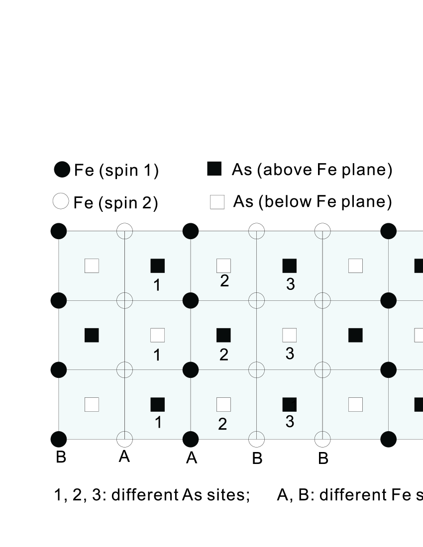
Figure 1: The structure of FeAs layer in the Q-SDW state showing the antiphase boundary in the center of the figure. Fe spin 1 (filled circle) and spin 2 (empty circle) have two different sites A (‘bulklike’) and B (‘boundary-like’). As above Fe plane (filled square) and below Fe plane (empty square) have three sites 1, 2, 3 whose local environments differ.

In this paper, we consider a class of magnetic arrangements derived from the stripe-like AFM phase: static periodic magnetic arrangements (SDWs) representing antiphase boundaries that require doubled, quadrupled, and octupled supercells. We denote these orders as D-SDW, Q-SDW and O-SDW, respectively. Figure 1 shows the magnetic arrangements of Fe in the Q-SDW phase. Its unit cell is a 4$\times$1$\times$1 supercell of the SDW unit cell. Antiphase boundaries occur at the edge and the center of its unit cell along a-axis (antiparallel/alternating Fe spins), the same as in the D-SDW and O-SDW states, the unit cells of which are 2$\times$1$\times$1 and 8$\times$1$\times$1 supercells of the SDW unit cell, respectively. The D-SDW phase can also be viewed as a double stripe SDW phase. Based on the results of these states, we consider the effect of antiphase boundary spin fluctuations in explaining various experimental results, which was discussed to some extent by Mazin and Johannes.Mazin-NP The antiphase magnetic boundaries we consider here are the simplest possible and yet explain semiquantitatively many experimental results by assuming that the dynamic average over antiphase magnetic boundaries can be modeled by averaging over several model antiphase boundaries. Our picture presumes that the antiphase boundary within the magnetically ordered state is in some sense a representative spin excitation in the FeAs-based compounds.

The calculations are done using the linear augmented plane wave (LAPW) method as implemented in the Wien2k code wien2k , with both PW91PW91 and PBEPBE exchange-correlaton (XC) potentials. Several results have been double checked using the full potential local orbital (FPLO) i codefplo1 ; fplo2 with PW91 XC potential.

II LDA VS. GGA

Whereas the local density approximation (LDA) for the exchange-correlation (XC) potential usually obtains internal coordinates accurately, it has been foundseb-njp ; GGA-magnetism that LDA makes unusually large errors when predicting the As height $z$(As) in these compounds in either nonmagnetic (NM) or SDW states. The generalized gradient approximation (GGA) makes similar errors in the NM state, however, GGA predicts very good values of $z$(As) in the SDW phase, as shown in Fig. 2. One drawback of GGA is that it enhances magnetismGGA-magnetism ; seb-njp in these compounds over the LDA prediction, which is already too large compared to its observed value. For example, using experimental structural parameters, GGA (PBE) gives a Fe spin magnetic moment larger than LDA (PW91) by 0.3 $\mu$_B in the SDW state, and more than 0.6 $\mu$_B in the D-SDW state. The magnetic moment changes the charge density, roughly in proportion to the moment. For this reason, we have used Wien2K with PW91 (LDA) XC functional with its more reasonable moments to calculate the EFG and hyperfine field using experimental structural parameters. We note that PBE and PW91 produce about the same EFG in the NM state.

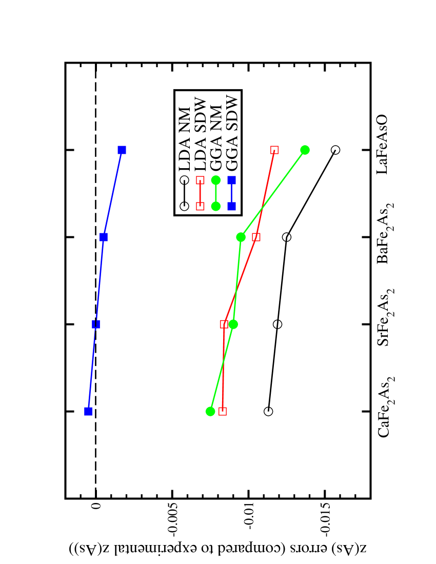
Figure 2: The calculated errors of z(As) compared to experimental values in the NM and SDW states when using LDA (PW91) and GGA (PBE) XC functionals in CaFe₂As₂, SrFe₂As₂, BaFe₂As₂, and LaFeAsO.

III The magnetic moment and hyperfine field of iron

In the various antiphase boundary SDW states, the Fe atoms can assume two different characters: high-spin A site away from the antiphase boundaries and low-spin B site at the antiphase boundaries, as shown in Fig. 1. The Fe atoms with the same site (A or B) in these states have about the same magnetic moment and hyperfine field. For example, in BaFe₂As₂ in the static Q-SDW state, the spin magnetic moment and hyperfine field for Fe at A site are 1.59 $\mu$_B and 12.6 T, and for Fe at B site are 0.83 $\mu$_B and 6.2 T. In the O-SDW state, the spin magnetic moments and hyperfine fields for the three (slightly different) A sites are 1.59, 1.60, 1.67 $\mu$_B and 12.6, 13.5, 1.37 T, respectively, and are 0.83 $\mu$_B and 6.1 T for Fe at B site.

As mentioned above, there are significant differences of the ordered magnetic moment of Fe in the SDW state between calculated values and values observed in neutron scattering (diffraction) experiments and/or Mössbauer experiments. Table 1 shows Fe spin magnetic moment and hyperfine field in the SDW and static D-SDW state calculated by FPLO7 and Wien2K using PW91 XC functional.

Table 1: The experimental magnetic moment of Fe m_Fe (in unit of $\mu$_B) and the hyperfine field B_hf (in unit of Tesla) for Fe, and values calculated in the SDW and D-SDW ordered phases, using Wien2K with PW91 for the $M$Fe₂As₂ ($M$=Ba, Sr, Ca), LaFeAsO and SrFeAsF compounds. The experimental values are in all cases much closer to the D-SDW values (with its maximally dense antiphase boundaries) than to the SDW values. Cruz-La ; Klauss-La-FeEFG ; Goldman-Ca ; Su-Ba ; Zhao-Sr ; Ba-FeEFG ; Sr-FeEFG ; SrF-FeEFG For the Fe magnetic moment, results from both FPLO (denoted as FP) and Wien2k(denoted as WK) are given. Because these methods (and other methods) differ somewhat in their assignment of the moment to an Fe atom, the difference gives some indication of how strictly a value should be presumed.

	exp		SDW			D-SDW
compound	mFe	Bhf	mFe		Bhf	mFe		Bhf
			FP	WK	WK	FP	WK	WK
BaFe2As2	0.8	5.5	1.78	1.65	13.6	0.90	0.80	5.4
SrFe2As2	0.94	8.9	1.80	1.68	13.9	0.98	0.91	6.1
CaFe2As2	0.8	–	1.63	1.53	12.4	0.77	0.71	4.7
LaFeAsO	0.36	–	1.87	1.77	14.9	0.50	0.48	3.6
SrFeAsF	—	4.8	–	1.66	14.5	—	0.32	2.3

IV Energy differences

Since Fe atoms in all these antiphase boundary SDW states have basically two spin states (high-spin state at A sites and low-spin state at B sites), in a local moment picture one might expect that energy differences could be related to just the two corresponding energies. From our comparison of energies we have found that this picture gives a useful account of the energetic differences.

The SDW and the D-SDW state are the simple cells in this regard. The former doesn’t have any low spin Fe and the latter doesn’t have any high spin Fe, so these two define the high spin (low energy) and low spin (high energy) “states” of the Fe atom. Table 2 shows the total energies per Fe (in meV) of the magnetic phases compared to the non-magnetic stater, for BaFe₂As₂, SrFe₂As₂, CaFe₂As₂, LaFeAsO and SrFeAsF. The high spin and low spin energies vary from system to system. The energy of the Q-SDW state has also been calculated, and it can be compared with the average of high spin and low spin moment energies (last column in Table 2). The reasonable agreement indicates that corrections beyond this simple picture are minor.

The energy cost to create an antiphase boundary is (roughly) simply the cost of two extra low spin Fe atoms versus the high spin that would result without the antiphase boundary. This difference is found to vary by over a factor of two, in the range of 40-90 meV per Fe for this set of five compounds. The reason for the variation is not apparent; for example, it is not directly proportional to the Fe moment (or its square).

Table 2: Calculated total energies (meV/Fe) compared to NM state of the various SDW states (SDW, D-SDW, Q-SDW) in the $M$Fe₂As₂ ($M$=Ba, Sr, Ca), LaFeAsO and SrFeAsF compounds. The energy tabulated in the last column, labeled Q^′, is the average of the high spin (SDW) and low spin (D-SDW) energies. illustrating that the energy of the Q-SDW ordered phase follows this average reasonably well. The level of agreement indicates to what degree ‘high spin’ and ‘low spin’ is a reasonable picture of the energetics at an antiphase boundary.

compound	SDW	D	Q	Q′
BaFe2As2	-73	-6	-36	-39
SrFe2As2	-91	-11	-46	-51
CaFe2As2	-66	-8	-33	-37
LaFeAsO	-143	-61	-94	-102
SrFeAsF	-73	0	-40	-37

Analogous calculations were also carried out for the large O-SDW cell for BaFe₂As₂. As for the other compounds and antiphase supercells, the Fe moments could be characterized by a low spin atom at the boundary and high spin Fe elsewhere. The energy could also be accounted for similarly, analogously to Table 2.

V The Electric Field Gradient

The EFG at the nucleus of an atom is sensitive to the anisotropy of the electron charge distribution around the atom. A magnitude and/or symmetry change of the EFG implies the local environment around the atom changes, which can be caused by changes in bonding, structure, or magnetic ordering. In BaFe₂As₂ during the simultaneously structure transition from tetragonal to orthorhombic and magnetic order transition from non-magnetic to SDW order at about 135 K, the EFG component V_c along the crystal c-axis drops rapidly by 10$\%$ and the asymmetry parameter $\eta=\frac{|V_{a}-V_{b}|}{|V_{c}|}$ jumps from zero to larger than one, indicating the principle axis for the largest component V_zz is changed from along c-axis to in the ab plane.Kitagawa-Ba-AsEFG The abrupt EFG change reflects a large change in the electron charge distribution around As sites and highly anisotropic charge distribution in the ab plane. A similar thing happens in CaFe₂As₂ except that the V_c component of CaFe₂As₂ in the non-magnetic state is five times that in BaFe₂As₂, and doubles its value at the structural and magnetic transition at 167 K when it goes to the SDW phase.Baek-Ca-AsEFG The different behaviour of the EFG change across the phase transition in BaFe₂As₂ and CaFe₂As₂ may be due to the out-of-plane alkaline-earth atom (Ba and Ca in this case), which influences the charge distribution around As atoms. It also indicates that three dimensionality is more important in $M$Fe₂As₂ than in $R$FeAsO, which is evident in the layer distance of the FeAs layers reflected in the c lattice constant of these compounds. The c lattice constant of CaFe₂As₂ is significantly smaller than BaFe₂As₂, so that the interlayer interaction of the FeAs layers is stronger in CaFe₂As₂, therefore the charge distribution in CaFe₂As₂ is more three dimensional like than in BaFe₂As₂, which can be clearly seen in their Fermi surfaces (not shown).

V.1 EFG of As atoms

The EFG of As can be obtained from the quadrupole frequency in nuclear quadrupolar resonance (NQR) measurement in nuclear magnetic resonance (NMR) experiment. The NQR frequency can be written as

$${\nu_{Q}=\frac{3eQV_{zz}(1+\eta^{2}/3)^{1/2}}{2I(2I-1)h}},$$ (1)

where Q ($\sim$ 0.3b, b=10^-24 cm²) is the ⁷⁵As quadrupolar moment, V_zz is the zz component of As EFG,

$$\eta=\frac{|V_{xx}-V_{yy}|}{|V_{zz}|}$$ (2)

is the asymmetry parameter of the EFG, I=3/2 is the ⁷⁵As nuclear spin, $h$ is the Planck constant. In LaO_0.9F_0.1FeAs, Grafe et al.EFG-LaAs reported $\nu$_Q=10.9 MHz, and $\eta$=0.1, which gives V_zz $\sim$ 3.00 $\times$ 10²¹ V/m². (Note: for the value of EFG, the unit 10²¹ V/m² is commonly used, and we will adopt this unit for all EFG values below) The experimental value 3.0 agrees satisfactorily with our resultseb-njp of 2.7 calculated by Wien2K code.

In BaFe₂As₂ and CaFe₂As₂, NMR experiments suggest the V_c component of the EFGs of As are 0.83 and 3.39 respectively at high temperature in the NM states,Kitagawa-Ba-AsEFG ; Baek-Ca-AsEFG while our calculated values are 1.02 and 2.35, respectively. The difference is in the right direction and right order of magnitude though not quantitatively accurate. However, the EFGs calculated in the SDW state don’t match experimental observations at all. In BaFe₂As₂ from 135 K down to very low temperature, V_c remains around 0.62 and $\eta=\frac{|V_{a}-V_{b}|}{|V_{c}|}$ changes from 0.9 to 1.2. Our calculated results in the SDW state gives V_a=1.34, V_b=-1.47, and V_c=-0.13, which gives $\eta$ $\approx$ 20. The calculated results substantially underestimate V_c and overemphasize the anisotropy in the ab plane.

We now consider whether these discrepancies can be clarified if antiphase boundary is considered. In the static D-SDW, Q-SDW and O-SDW states, the surrounding environment of As sites change. Depending on the magnitudes (high spin or low spin) and directions (parallel or antiparallel) of the spins of their nearest and next nearest neighboring Fe atoms, As atoms generally have three different sites (1, 2, and 3) as shown in Fig. 1. In the static D-SDW state, As atoms have similar site 1^′ and 3^′. As shown in Table 3, the calculated quantities for these states cannot directly explain the experimental observed values neither.

However, they may be understandable if the antiphase boundary is dynamic, i.e., any As atom in a given measurement can change from site 1 to site 2 and/or site 3, when its nearby Fe atoms flip their spin directions. These time fluctuations have be represented by an average over configurations, and we consider briefly what arises from a configuration average over our SDW phase and three short-period ordered cells (having different densities of anti-phase boundaries). In the O-SDW state, for example, if an As samples 25$\%$, 25$\%$ and 50$\%$ “time” as As sites 1, 2 and 3, respectively during the experimental measurement, then the expectation values are V_a=0.99, V_b=-0.29, V_c=-0.71, $\eta$=1.80, B_hf=1.43 T. This simple consideration already match much better with experimentalKitagawa-Ba-AsEFG observed V_c $\sim$ 0.62, H_in=1.4 T, except $\eta$ which is around 1.2. The actual situation could be much more complicated, being an average over all the sites in all the static D-SDW, Q-SDW and O-SDW states, and other more complicated states. Considering the relatively small differences of the EFGs at the same site for Q-SDW and O-SDW order, As sites in other static antiphase boundary SDW states should be able to be classified to site 1, 2 and 3 as in the Q-SDW and O-SDW states.

Table 3: The calculated EFG component V_a, V_b, V_c (in unit of 10²¹ V/m²) , the asymmetry parameter $\eta$, spin magnetic moment of As ($\mu$_B), hyperfine field at the As nuclei (Tesla) of BaFe₂As₂ in the SDW, D-SDW, Q-SDW and O-SDW states. Experimentally, V_c is around 0.62, $\eta$ is in the range of 0.9 to 1.2, and the internal field at As site parallel to c axis is about 1.4 T.Kitagawa-Ba-AsEFG See text for notation.

state	site	Va	Vb	Vc	$\eta$	Bhf
SDW	1	1.21	-1.32	0.11	23.0	0
D-SDW	1′	0.63	0.07	-0.70	0.8	0
	3′	0.66	0.37	-1.03	0.28	2.1
Q-SDW	1	1.17	-1.38	0.21	12.1	0
	2	0.99	-0.72	-0.27	6.33	1.0
	3	0.90	0.51	-1.41	0.28	2.1
O-SDW	1	1.25	-1.44	0.19	14.2	0
	2	0.98	-0.71	-0.27	6.26	1.1
	3	0.87	0.50	-1.37	0.27	2.3

V.2 EFG of Fe atoms

The EFG of Fe can be obtained from the electric quadrupole splitting parameter derived from Mössbauer measurements. The electric quadrupole splitting parameter can be written as

$${\Delta=\frac{3eQV_{zz}(1+\eta^{2}/3)^{1/2}}{2I(2I-1)}},$$ (3)

which equals E_γ$\Delta$E_Q/c, where Q $\sim$ 0.16b is the ⁵⁷Fe quadrupolar moment, E_γ is the energy of the $\gamma$ ray emitted by the ⁵⁷Co/Rh source, $\Delta$E_Q is the electric quadrupole splitting parameter from Mössbauer data given in the unit of speed, and c is the speed of light in vacuum. By fitting the Mössbauer spectra, one also obtains the isomer shift $\delta$ and average hyperfine field B_hf.

We consider whether the dynamic antiphase boundary spin fluctuation picture can also clarify the comparison between calculated and observed EFG of Fe. We take SrFe₂As₂ as an example. As shown in Table 4, in the NM state, the calculated value V_Q=0.98 agrees well with the V${}_{Q}\approx$ 0.83 at room temperature. V_Q calculated in the SDW state (0.68) agrees rather well with experimental value about 0.58 at 4.2 K. V_Q calculated in the D-SDW state (0.80) is somewhat larger than that in the SDW state, but not . Regarding EFG, the biggest difference between SDW and D-SDW is the asymmetry parameter–it is 0.61 in the SDW and only 0.11 in the latter. Further experiments are required to clarify this difference.

Table 4: The calculated EFG component V_a, V_b, V_c (in unit of 10²¹ V/m²) , the asymmetry parameter $\eta$=$|$V_xx-V_yy$|$/$|$V_zz$|$ (here $|$V_zz$|$ $>$ $|$V_xx$|$ and $|$V_yy$|$), V_Q=$|$V_zz$|$/(1+$\eta$²/3)^1/2 of Fe in SrFe₂As₂ in the NM, SDW, D-SDW, Q-SDW and O-SDW states. Experimentally, V_Q is around 0.83 at room temperature in the non-magnetic state, and it is about 0.58 at 4.2 K.Sr-FeEFG

state	site	Va	Vb	Vc	$\eta$	VQ
NM	0	-0.49	-0.49	0.98	0	0.98
SDW	A	-0.58	-0.14	0.72	0.61	0.68
D-SDW	B	-0.30	-0.51	0.81	0.26	0.80
Q-SDW	A	-0.63	-0.06	0.69	0.83	0.62
	B	-0.56	-0.49	1.05	0.07	1.05

VI Summary

Experiments generally indicate that an itinerant magnetic moment, magnetic (SDW) instability, and spin fluctuations are common features of the Fe-based superconductors. In this paper, we have studied the energetics, charge density distribution (through calculation of the electric field gradients, hyperfine fields and magnetic moments) for ordered supercells with varying densities of antiphase magnetic boundaries, namely the SDW, D-SDW, Q-SDW and (for very limitied cases) O-SDW phases. Supposing dynamic magnetic antiphase boundaries are present, and that the spectroscopic experiments average over them, we can begin to clarify several seemingly contradictory experimental and computational results.

Our calculations tend to support the idea that antiphase boundary magnetic configurations can be important in understanding data. The fact that the decrease in moment is confined to the antiphase boundary Fe atom does not mean that a local moment picture is appropriate; in fact, exactly this same type of local spin density calculations provide a description of magnetic interaction that is at odds with a local moment picture.johannes09 The calculated energy cost to create an antiphase boundary is however rather high for the cases we have considered, and this value would seem to restrict formation of antiphase boundaries at temperatures of interest. Calculations that treat actual disorder, and dynamics as well, would be very helpful in furthering understanding in this area.

VII Acknowledgments

This work was supported by DOE grant DE-FG02-04ER46111. We also acknowledge support from the France Berkeley Fund that enabled the initiation of this project.

References

- (1) Y. Kamihara, T. Watanabe, M. Hirano, and H. Hosono, J. Am. Chem. Soc. 130, 3296 (2008).
- (2) G. F. Chen, Z. Li, D. Wu, G. Li, W. Z. Hu, J. Dong, P. Zheng, J. L. Luo, and N. L. Wang, Phys. Rev. Lett. 100, 247002 (2008).
- (3) Z.-A. Ren, J. Yang, W. Lu, W. Yi, X.- L. Shen, Z.-C. Li, G.-C. Che, X.-L. Dong, L.-L. Sun, F. Zhou, and Z.-X. Zhao, Europhysics Letters 82 (2008) 57002
- (4) Z.-A. Ren, J. Yang, W. Lu, W. Yi, G.-C. Che, X.-L. Dong, L.-L. Sun, and Z.-X. Zhao, Materials Research Innovations 12, 105, (2008)
- (5) P. Cheng, L. Fang, H. Yang, X. Y. Zhu, G. Mu, H. Q. Luo, Z. S. Wang, and H.-H. Wen, Science in China G 51(6), 719-722(2008).
- (6) C. Wang, L. J. Li, S. Chi, Z. W. Zhu, Z. Ren, Y. K. Li, Y. T. Wang, X. Lin, Y. K. Luo, S. Jiang, X. F. Xu, G. H. Cao, and Z. A. Xu, Europhysics Letters 83, 67006 (2008).
- (7) Z.-A. Ren, W. Lu, J. Yang, W. Yi, X.-L. Shen, Z.-C. Li, G.-C. Che, X.-L. Dong, L.-L. Sun, F. Zhou, and Z.-X. Zhao, Chin. Phys. Lett. 25, 2215 (2008).
- (8) M. Rotter, M. Tegel, and D. Johrendt, Phys. Rev. Lett. 101, 107006 (2008).
- (9) K. Sasmal, B. Lv, B. Lorenz, A. M. Guloy, F. Chen, Y. Y. Xue, and C. W. Chu, Phys. Rev. Lett. 101, 107007 (2008)
- (10) M. S. Torikachvili, S. L. Bud’ko, N. Ni, and P. C. Canfield, Phys. Rev. Lett. 101, 057006 (2008).
- (11) J. H. Tapp, Z. J. Tang, B. Lv, K. Sasmal, B. Lorenz, P. C.W. Chu, and A. M. Guloy, Phys. Rev. B 78, 060505(R) (2008).
- (12) D. R. Parker, M. J. Pitcher, P. J. Baker, I. Franke, T. Lancaster, S. J. Blundell, and S. J. Clarke, Chem. Commun. (Cambridge) 2009, 2189.
- (13) S. Matsuishi, Y. Inoue, T. Nomura, M. Hirano, and H. Hosono, J. Phys. Soc. Jpn. 77, 113709 (2008).
- (14) C. de la Cruz, Q. Huang, J. W. Lynn, J. Li, W. R. II, J. L. Zarestky, H. A. Mook, G. F. Chen, J. L. Luo, and N. L. Wang, Nature 453, 899 (2008).
- (15) M. A. McGuire, A. D. Christianson, A. S. Sefat, B. C. Sales, M. D. Lumsden, R. Y. Jin, E. A. Payzant, D. Mandrus, Y. B. Luan, V. Keppens, V. Varadarajan, J. W. Brill, R. P. Hermann, M. T. Sougrati, F. Grandjean, and G. J. Long, Phys. Rev. B 78, 094517 (2008).
- (16) K. Kitagawa, N. Katayama, K. Ohgushi, M. Yoshida, and M. Takigawa, J. Phys. Soc. Jpn. 77, 114709 (2008).
- (17) S.-H. Baek, N. J. Curro, T. Klimczuk, E. D. Bauer, F. Ronning, and J. D. Thompson, Phys. Rev. B 79, 052504 (2009).
- (18) Z. P. Yin, S. Lebégue, M. J. Han, B. P. Neal, S. Y. Savrasov, and W. E. Pickett, Phys. Rev. Lett. 101, 047001 (2008).
- (19) T. Yildirim, Phys. Rev. Lett. 101, 057010 (2008).
- (20) D. J. Singh and M.-H. Du, Phys. Rev. Lett. 100, 237003 (2008).
- (21) S. Lebégue, Z. P. Yin, and W. E. Pickett, New J. Phys. 11, 025004 (2009).
- (22) I. I. Mazin, D. J. Singh, M. D. Johannes, and M. H. Du, Phys. Rev. Lett. 101, 057003 (2008).
- (23) F. Ma, Z.-Y. Lu, and T. Xiang, Phys. Rev. B 78, 224517 (2008).
- (24) I. I. Mazin, M. D. Johannes, L. Boeri, K. Koepernik, and D. J. Singh, Phys. Rev. B 78, 085104 (2008).
- (25) K. Haule, J. H. Shim, and G. Kotliar, Phys. Rev. Lett. 100, 226402 (2008).
- (26) Y. Su, P. Link, A. Schneidewind, T. Wolf, P. Adelmann, Y. Xiao, M. Meven, R. Mittal, M. Rotter, D. Johrendt, T. Brueckel, and M. Loewenhaupt, Phys. Rev. B 79, 064504 (2009).
- (27) J. Zhao, W. Ratcliff, J. W. Lynn, G. F. Chen, J. L. Luo, N. L. Wang, J. Hu, and P. Dai, Phys. Rev. B 78, 140504(R) (2008).
- (28) A.I. Goldman, D.N. Argyriou, B. Ouladdiaf, T. Chatterji, A. Kreyssig, S. Nandi, N. Ni, S. L. Bud’ko, P.C. Canfield, and R. J. McQueeney, Phys. Rev. B 78, 100506(R) (2008).
- (29) M. D. Johannes and I. I. Mazin, Phys. Rev. B 79, 220510(R) (2009).
- (30) S. Kitao, Y. Kobayashi, S. Higashitaniguchi, M. Saito, Y. Kamihara, M. Hirano, T. Mitsui, H. Hosono, and M. Seto, J. Phys. Soc. Jpn. 77 103706 (2008)
- (31) H.-H. Klauss, H. Luetkens, R. Klingeler, C. Hess, F.J. Litterst, M. Kraken, M. M. Korshunov, I. Eremin, S.-L. Drechsler, R. Khasanov, A. Amato, J. Hamann-Borrero, N. Leps, A. Kondrat, G. Behr, J. Werner, and B. Buchner, Phys. Rev. Lett. 101, 077005 (2008).
- (32) I. Nowik, I. Felner, V. P. S. Awana, A. Vajpayee, and H. Kishan, J. Phys.: Condens. Matter 20, 292201 (2008).
- (33) I. Nowik and I. Felner, J. Supercond. Nov. Magn. 21, 297 (2008).
- (34) M. Rotter, M. Tegel and D. Johrendt, I. Schellenberg, W. Hermes, and R. Pöttgen, Phys. Rev. B 78, 020503(R) (2008).
- (35) M. Tegel, M. Rotter, V. Weiss, F. M. Schappacher, R. Poettgen, and D. Johrendt, J. Phys.: Condens. Matter 20, 452201 (2008).
- (36) M. Tegel, S. Johansson, V. Weiss, I. Schellenberg, W. Hermes, R. Poettgen, and D. Johrendt Europhys. Lett. 84, 67007 (2008).
- (37) H.-J. Grafe, D. Paar, G. Lang, N. J. Curro, G. Behr, J. Werner, J. Hamann-Borrero, C. Hess, N. Leps, R. Klingeler, and B. Bchner, Phys. Rev. Lett. 101, 047003 (2008).
- (38) A. J. Drew, Ch. Niedermayer, P. J. Baker, F. L. Pratt, S. J. Blundell, T. Lancaster, R. H. Liu, G. Wu, X. H. Chen, I. Watanabe, V. K. Malik, A. Dubroka, M. Röessle, K. W. Kim, C. Baines, and C. Bernhard, Nature Mater. 8, 310 (2009).
- (39) W. Z. Hu, J. Dong, G. Li, Z. Li, P. Zheng, G. F. Chen, J. L. Luo, and N. L. Wang, Phys. Rev. Lett. 101, 257005 (2008).
- (40) K. Matan, R. Morinaga, K. Iida, and T. J. Sato, Phys. Rev. B 79, 054526 (2009).
- (41) R.A. Ewings, T.G. Perring, R.I. Bewley, T. Guidi, M.J. Pitcher, D.R. Parker, S.J. Clarke, and A.T. Boothroyd, Phys. Rev. B 78, 220501(R) (2008).
- (42) I. I. Mazin and M. D. Johannes, Nature Physics 5, 141-145 (2009).
- (43) P. Blaha, K. Schwarz, G. K. H. Madsen, D. Kvasnicka, and J. Luitz, WIEN2K,(K. Schwarz, Techn. Univ. Wien, Austria) (2001).
- (44) J. P. Perdew and Y. Wang, Phys. Rev. B 45, 13244 (1992).
- (45) J. P. Perdew, K. Burke, and M. Ernzerhof, Phys. Rev. Lett 77, 3865 (1996).
- (46) K. Koepernik and H. Eschrig, Phys. Rev. B 59, 1743 (1999).
- (47) K. Koepernik, B. Velicky, R. Hayn, and H. Eschrig, Phys. Rev. B 55, 5717 (1997).