Confinement effects on intermediate state flux patterns in mesoscopic type-I superconductors

Abstract

Intermediate state (IS) flux structures in mesoscopic type-I superconductors are investigated within the Ginzburg-Landau theory. In addition to well-established tubular and laminar structures, the strong confinement leads to the formation of (i) a phase of singly quantized vortices, which is typical for type-II superconductors and (ii) a ring of a normal domain at equilibrium. The stability region and the formation process of these IS flux structures are strongly influenced by the geometry of the sample.

Intermediate state (IS) of type-I superconductors has received a revival of interest in recent years Fidler ; pro2 as one of the rare systems where competing interactions lead to the formation of spatially modulated structures. This kind of complex structures have been observed in other systems like ferrofluids, amphiphilic monolayers and chemical reaction-diffusion systems Seul . Analogies to type-I superconductors also extend to astrophysics Buckley .

IS flux structures can be described theoretically assuming parallel stripes of normal and superconducting (SC) domains landau or a periodic array of multiquanta flux tubes goren . The tubular structure is more mobile, while the laminar structure is topologically constrained Hoberg and transition between these states occurs for larger volume fraction of normal domains cebers . However, these regular patterns are rarely seen in experiment huebener . Instead, much more complex flux structures – highly branched and intricate fingered patterns of flux domains – are often observed huebener ; faber ; miller ; kiendl ; pro1 ; pro2 . In addition, type-I superconductors show clear hysteresis – flux tubes are obtained during magnetic field penetration and laminar structures are formed during magnetic field expulsion pro1 ; Velez , suggesting that the system gets stuck in a metastable state, i.e., the sample is not in thermodynamic equilibrium. Zero-bulk pinning pro2 superconducting spheres and cones show no hysteresis with flux tubes dominating the IS. With increasing applied magnetic field, a new phase – a suprafroth – is formed Fidler , which represents neither tubular nor laminar structure.

The behavior becomes richer in the mesoscopic regime, where, in addition to the competition between the magnetic energy that favors the formation of small normal domains and the positive surface energy that tends to form large domains, confinement effects become important. In type-II superconductors confinement strongly influences the distribution of vortices leading to, e.g., the formation of giant vortices kanda and symmetry induced vortex-antivortex pairs chibo . Misko et al., stabilized such vortex-antivortex patterns in a long type-I superconducting prism with triangular cross section slava , due to the competition between vortex-antivortex repulsion and finite size effects. However, their study was limited to a very narrow range of applied magnetic field. Our main goal in this paper is a systematic study of ground state flux structures in mesoscopic type-I superconductors. We also address another important problem not yet studied neither experimentally nor theoretically: the effect of sample geometry on these mesoscopic IS patterns.

From the theoretical point of view, the difficulty of modeling the IS comes from the 3D nature of the magnetic interaction of the domains. Therefore, approximate expressions are usually used for the magnetic energy. goren ; goldstein ; dorsey ; cebers In our approach we used the Ginzburg-Landau (GL) theory, where no approximation for the magnetic energy is used and the structure of the domains is not predetermined. We solve the GL equations for the order parameter $\Psi$ and the vector potential ${\bf A}$:

$$(-i\nabla-{\bf A})^{2}\Psi=(1-|\Psi|^{2})\Psi,$$ (1)

$$-\kappa^{2}\nabla\times\nabla\times{\bf A}=\textrm{Im}(\Psi^{*}\nabla\Psi)-|\Psi|^{2}{\bf A},$$ (2)

where $\kappa$ is the GL parameter. Here, the distance is measured in units of the coherence length $\xi$, the vector potential $\vec{A}$ in $c\hbar/2e\xi$, and the order parameter $\Psi$ in $\sqrt{-\alpha/\beta}$ with $\alpha$, $\beta$ being the GL coefficients. Following the numerical approach of Ref. schw , we apply a finite-difference representation for the order parameter and the vector potential on a uniform 3D Cartesian space grid (up to $256\times 256\times 256$ grid points). $\Psi$ satisfies the boundary condition $(-i\nabla-{\bf A})\Psi|_{n}=0$ at the sample surface and far away from the superconductor ${\bf A}$ is determined by the external applied field. The simulations of the IS are conducted in i) field sweep up: we started from the full Meissner state ($|\Psi|=1$) and slowly increased the magnetic field, after reaching the stationary state; ii) field sweep down: we started simulations with $|\Psi|=0$ and $H>H_{c}$ and decreased the field with small steps; and iii) field cooled simulations starting from random initial conditions for each value of the applied field.

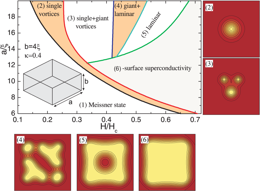
Figure 1: (Color online) The ground state flux structures for a rectangular prism of size $a$ and height $b$ (see the inset) as a function of $a$ and the applied magnetic field $H$ for $b=4\xi$ and $\kappa=0.4$. The insets (2-6) denote the Cooper-pair density plots [red (dark gray)/yellow (light gray) corresponds to high/low $|\psi|^{2}$] of the corresponding states.

Equilibrium flux structures. – As a representative example of mesoscopic type-I superconductors, we studied IS flux structures in a rectangular prism of size $a$ and height $b$ exposed to a homogeneous field $H$ (see insets of Fig. 1). We constructed the equilibrium phase diagram as a function of $a$ and $H$ for $\kappa=0.4$ and $b=4\xi$ as shown in Fig. 1. The ground state was found from the field cooled simulations by comparing the energies of all found states for given magnetic field and sample parameters. The Meissner state (region 1) is found at small fields and the stability of this phase increases to larger fields with decreasing sample size. The most prominent feature of this phase diagram is the existence of region 2 where singly quantized fluxes (i.e., individual vortices) are nucleated in the sample (see inset 2). Note that this state is typical for type-II superconductors and was never found in bulk type-I samples hernandez ; pro1 ; pro2 , where the energy of singly quantized vortices is larger than the energy of multiply quantized flux tubes. At higher fields individual vortices are too close to each other and giant vortices nucleate together with individual vortices (region 3) as illustrated by inset 3 of Fig. 1. In region 4 laminar-like structures start to form in combination with flux tubes (inset 4). Such laminar-like structures are obtained for larger $a$, usually in the form of a ring of normal domain (inset 5). This novel state is a consequence of strong confinement imposed by the sample surface and resembles recently found suprafroth in macroscopic SC spheres Fidler . Surface superconductivity (region 6) is formed before the system transits to the normal state (inset 6). Notice also that, we did not find branching of normal domains, which occurs in very thick samples huebener . From this phase diagram we notice that the ground state flux structures in mesoscopic type-I superconductors do not depend only on the applied magnetic field (as in the case of bulk superconductors cebers ), but also on the confinement due to the finite size of the sample. The latter leads to the formation of singly quantized flux tubes and a ring of normal domain.

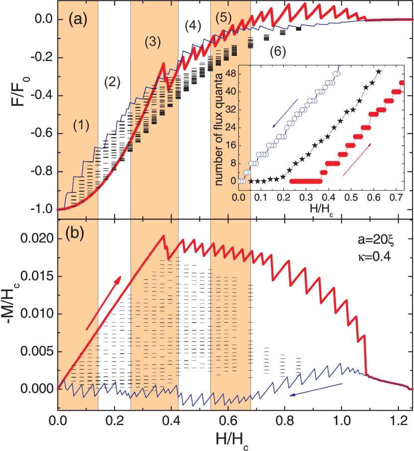
Figure 2: (Color online) The free energy (a) and the magnetization (b) as a function of the applied magnetic field for a superconducting cube of size $a=20\xi$ and for $\kappa=0.4$. Thick red (blue thin) curves are the results obtained when increasing (decreasing) the magnetic field and the symbols (hyphens) show the results of field cooling simulations. The inset shows the total number of flux in the sample as a function of the applied field obtained during field sweep up (filled red circles), field sweep down (open blue circles) and of the lowest energy state from field cooled (stars) simulations.

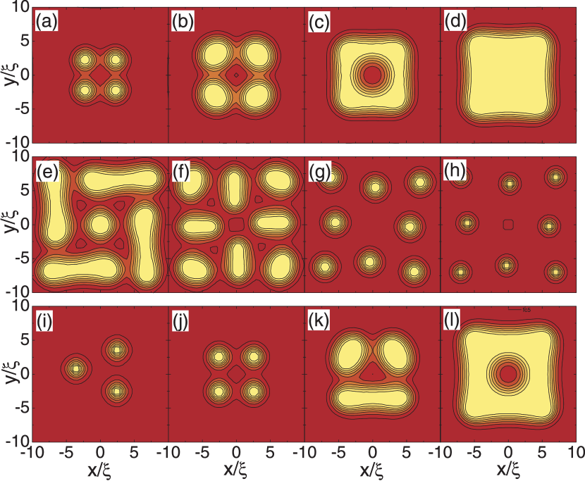
Figure 3: (Color online) Contour plots of the Cooper pair density $|\psi|^{2}$ in the middle plane of the cube obtained during magnetic field sweep up (a-d), down (e-h) and in field cooling regime (the ground state) (i-l) at the applied fields $H/H_{c}$=: 0.44 (a), 0.52 (b), 0.55 (c), 0.66 (d), 0.43 (e), 0.37 (f), 0.15 (g), 0.08 (h), 0.17 (i), 0.28 (j), 0.48 (k), and 0.57 (l). The number of fluxoids $N$ is: 8 (a), 20 (b), 28 (c), 36 (d), 48 (e), 40 (f), 16 (g), 8 (h), 3 (i), 8 (j), 22 (k), and 40 (l).

Effect of sample geometry. An important factor that influences the formation of IS patterns is the sample shape and geometry pro2 ; fortini ; castro . For example, a recent experiment showed pro2 that zero-bulk pinning discs and slabs show hysteretic behavior – flux tubes appear on magnetic field penetration and lamellae on flux exit. Spheres and cones show no hysteresis with flux tubes dominating the intermediate field region. In what follows, we study the influence of the sample geometry on the IS flux structures, as an example of a superconducting cube and sphere with the same superconducting volume $V$. Figure 2 shows the free energy (in units of $F_{0}=H_{c}^{2}V/8\pi$) (a) and the magnetization (b) of a cube with size $a=20\xi$ as a function of the applied magnetic field. In the field sweep up regime (thick red curve), the sample is in the Meissner state up to $H_{p}=0.38H_{c}$ – the penetration of flux is prohibited by the surface barrier. When the penetration field $H_{p}$ is reached four flux quanta enter the sample forming one circular flux tube or a giant vortex. With a small increase of the field, 4 flux quanta enter forming 4 giant vortices, each with vorticity 2 (Fig. 3(a)). The strong confinement in the mesoscopic regime prevents the formation of hexagonal structures and we usually obtain square symmetric structures (Figs. 3(a,b,e-h)). Previous studies showed that with increasing field magnetic flux enters the sample in the form of tubes pro1 which were believed to be due to the presence of a surface barrier fortini . The smallness of our sample enhances the effect and only a single flux quantum enters through each side of the cube and join the existing normal domains. In this way, the square symmetry of the flux structure remains unaltered and only the number of flux quanta in each normal domain increases (Fig. 3(b)). With further increasing the field a ring of normal phase is formed surrounding a SC domain (Fig. 3(c)). This ring structure closes at $H=0.66H_{c}$ and only surface superconductivity (Fig. 3(d)) remains until the system transits to the normal state.

The topological hysteresis in the IS flux structures in macroscopic samples pro2 was previously explained by the presence of a surface barrier which is absent in decreasing fields brandt – a large number of lamellae are connected to the sample edge during flux exit, allowing the magnetic flux to exit continuously, while these large normal domains are broken into smaller pieces during flux penetration. Thin blue curve in Fig. 2(a) shows the free energy of the cube when decreasing the magnetic field $H$. Surface superconductivity first nucleates resulting in a narrow flux-free zone, as obtained in the experiment valko . With further decreasing $H$, a SC phase nucleates in the central part of the sample, embedded within the normal phase (similar to the state in Fig. 3(c)) reducing the total number of flux quanta (see the inset of Fig. 2(a)). At $H=0.43H_{c}$ the long normal domain breaks down into 4 smaller domains that are arranged into a square symmetric structure (Fig. 3(e)). When reducing the magnetic field further the length of the normal lamellae decreases until they are reduced to flux tubes (Fig. 3(f)). The expulsion of flux occurs in such a way that only part of the tubes leave the sample and the number of normal domains remain unchanged (Fig. 3(g)). The expulsion of the flux occurs with smaller steps compared to the case of magnetic field sweep up. Further decreasing the field leads to the formation of patterns containing singly-quantized vortices (Fig. 3(h)). At $H=0.023H_{c}$ the magnetic field is totally expelled and the system transits to the Meissner state. Notice that the square symmetry of the IS flux structures is always preserved, while in large samples the square symmetry is broken when decreasing the field hernandez . This difference is a consequence of stronger confinement (surface barrier) in mesoscopic samples.

From Fig. 2(a) it is clear that the ground state of the sample is not reached during both field sweep up and down (except for the Meissner phase) – the system is locked in higher energy metastable states. The ground state can be obtained during field cooling simulations, the results of which are shown by symbols in Fig. 2. As seen from this figure the system can nucleate in many different (meta)stable states when starting from different random initial conditions. The total number of flux quanta $N$ inside the sample is smaller during magnetic field sweep up (solid circles) and it is much larger when decreasing the field (open circles) as compared to the one in the ground state (stars) (see the inset of Fig. 2(a)). The existence of such superheated and supercooled states results in a large hysteresis in the magnetization curve gourdon . The magnetization of the sample, defined as the flux expelled from the sample $M=(\langle H\rangle-H)/4\pi$, where $\langle H\rangle$ is averaged over the sample volume magnetic field, schw is shown in Fig. 2(b). Each jump in the magnetization curve corresponds to a transition between different flux states. The difficulty of expelling flux results in a positive magnetization in decreasing field (thin blue curve in Fig. 2(b)). The hysteresis disappears at very small fields, and at larger magnetic fields when only surface superconductivity exists. Transition from the tubular state to the laminar-like state (4) occurs at $H$$\simeq$$0.42H_{c}$, which is slightly larger than the field ($H\simeq 0.3H_{c}$) corresponding to the transition between tubular and laminar states in bulk samples cebers . The corresponding ground state flux structures are shown in Figs. 3(i-l).

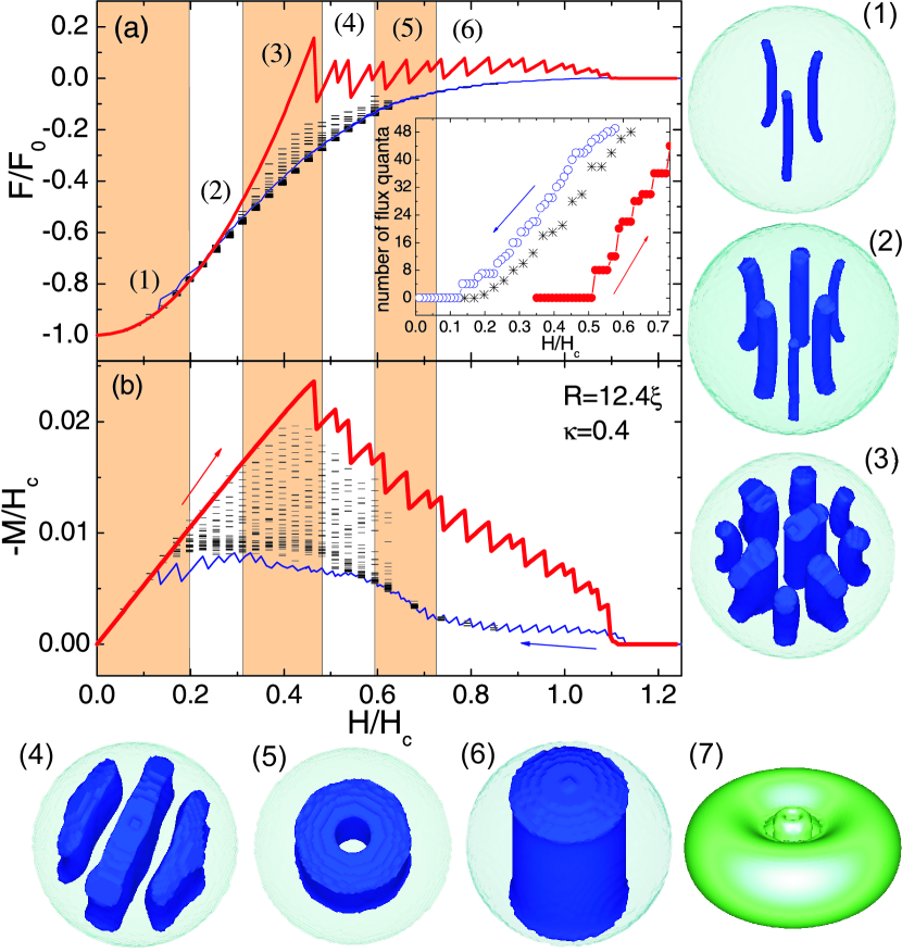
Figure 4: (Color online) The same as Fig. 2, but for a sphere of radius $R=12.4\xi$. Isosurface plots show the ground state flux structures in the sphere at the magnetic fields: $H=0.23H_{c}$ (N=3) (1), $H=0.31H_{c}$ (N=10) (2), $H=0.51H_{c}$ (N=38) (3), $H=0.59H_{c}$ (N=46) (4), $H=0.62H_{c}$ (N=48) (5) and $H=0.73H_{c}$ (N=55) (6). Light (dark) blue corresponds to superconducting (normal) region. Inset 7 shows the magnetic field distribution around the sphere corresponding to the state shown in inset 5.

Next, we contrast the results of the cube to the case of a mesoscopic sphere. Figure 4 shows the free energy (a) and magnetization (b) vs. the magnetic field $H$ for a sphere of radius $R=12.4\xi$. The effect of the sample geometry leads to the following differences. First, the Meissner effect becomes more pronounced leading to a larger first penetration field ($H_{p}=0.47H_{c}$) (thick red curve) fortini ; castro . Due to the nonzero demagnetization factor of the sphere the magnetic field is strongly disturbed near the sample boundary, resembling the magnetic field profile of a dipole (see inset 7 in Fig. 4). The jump in the total number of flux quanta becomes larger as compared to the case of the cube (compare filled circles in the insets of Figs. 2(a) and 4(a)). Second, the number of possible meta(stable) states (hyphens in Fig. 4(a)) is substantially smaller in field cooling simulations, especially at low and high fields. Only at midrange fields a larger number of metastable states is found, but energy levels are very close to each other. The most interesting results are found for the magnetic field sweep down regime: the jumps in the free energy (and magnetization) curve (thin blue curve) are much smaller, leading to an almost continuous change in the number of flux quanta. Moreover, the system follows very closely the ground state, with only a few more flux quanta trapped inside the sample (compare open circles and stars in the inset of Fig. 4(a)). As a result of all this, the magnetic hysteresis is smaller and no paramagnetic effect is observed (Fig. 4(b)). These results allow us to conclude that the surface barrier for penetration of magnetic field in a sphere is larger compared to the one in flat samples (i.e., a cube), while it is strongly reduced during flux expulsion. However, in contrast to the macroscopic sphere Velez , there is no complete disappearance of the surface barrier in our mesoscopic sphere. Isosurface plots (1-6) in Fig. 4 shows the ground state flux structures of the sphere for different magnetic field values. At small fields only singly quantized vortices are found in the ground state (inset 1) and, with increasing $H$, giant vortices appear (inset 2). Due to the boundary condition the flux tubes should be perpendicular to the surface of the sample, leading to the curvature of flux tubes. Laminar-like structures first appear in the form of deformed flux tubes (inset 3) and radially oriented stripes (inset 4) or a ring of normal domain (inset 5). And, finally, we arrive at the surface superconductivity state with one big central normal domain (inset 6).

Concluding, a remarkable variety of possible flux structures in the IS of type-I superconductors are found in the mesoscopic regime. For example, single-quantized flux tubes (vortices) are stabilized due to the confinement imposed by the sample surface. The latter also leads to the formation of a ring of normal domain at larger applied fields. All these findings are summarized into the phase diagram (Fig. 1). The transition point between different flux structures depends on the geometry of the sample which is related to the surface barrier for flux entry and exit. Regardless of the sample geometry the ground state of the IS at low fields consists of flux tubes and the transition to the laminar-like state takes place at larger magnetic fields.

This work was supported by the Belgian Science Policy (IAP) and the collaborative project FWO-MINCyT (FW/08/01). G.R.B. acknowledges support from FWO-Vlaanderen.

References

- (1) A.F. Fidler et al., Nature Physics 4, 327 (2008).
- (2) R. Prozorov, Phys. Rev. Lett. 98, 257001 (2007).
- (3) M. Seul and D. Andelman, Science 267, 476 (1995).
- (4) K.B.W. Buckley et al., Phys. Rev. Lett. 92, 151102 (2004).
- (5) L.D. Landau, Zh. Eksp. Teor. Fiz. 7, 371 (1937).
- (6) R.N. Goren and M. Tinkham, J. Low Temp. Phys. 5 465 (1971).
- (7) R.P. Huebener, Magnetic Flux Structures in Superconductors (Springer-Verlag, New York, 1979).
- (8) T.E. Faber, Proc. R. Soc. London A 248, 460 (1958).
- (9) R.E. Miller and G.D. Cody, Phys. Rev. 173, 494 (1968).
- (10) A. Kiendl and H. Kirchner, J. Low Temp. Phys. 14, 349 (1974).
- (11) R. Prozorov et al., Phys. Rev. B 72, 212508 (2005).
- (12) S. Vlez et al., Phys. Rev. B 78, 134501 (2008).
- (13) J.B. Hoberg and R. Prozorov, Phys. Rev. B 78, 104511 (2008).
- (14) A. Cbers et al., Phys. Rev. B 72, 014513 (2005).
- (15) A. Kanda et al., Phys. Rev. Lett. 93, 257002 (2004).
- (16) L.F. Chibotaru et al., Nature (London) 408, 833 (2000).
- (17) V.R. Misko et al., Phys. Rev. Lett. 90, 147003 (2003).
- (18) R.E. Goldstein et al., Phys. Rev. Lett. 76, 3818 (1996).
- (19) A.T. Dorsey and R.E. Goldstein, Phys. Rev. B 57, 3058 (1998).
- (20) V.A. Schweigert et al., Phys. Rev. Lett. 81, 2783 (1998).
- (21) A. Fortini and E. Paumier, Phys. Rev. B 14, 55 (1976).
- (22) E.H. Brandt, Phys. Rev. B 60, 11939 (1999).
- (23) P. Valko et al., Phys. Rev. B 75, 140504(R) (2007).
- (24) A.D. Hernandez and D. Dominguez, Phys. Rev. B 72, 020505(R) (2005).
- (25) C. Gourdon et al., Phys. Rev. Lett. 96, 087002 (2006).
- (26) H. Castro et al., Phys. Rev. B 59, 596 (1999).