A correlation between the spectral and timing properties of AGN

Abstract

Context. We present the results from a combined study of the average X–ray spectral and timing properties of 14 nearby AGN.

Aims. We investigate whether a “spectral-timing” AGN correlation exists, similar to the one observed in Cyg X-1, compare the two correlations, and constrain possible physical mechanisms responsible for the X–ray emission in compact, accreting objects.

Methods. For 11 of the sources in the sample, we used all the available data from the RXTE archive, which were taken until the end of 2006. There are 7795 RXTE observations in total for these AGN, obtained over a period of $\sim 7-11$ years. We extracted their 3–20 keV spectra and fitted them with a simple power-law model, modified by the presence of a Gaussian line (at 6.4 keV) and cold absorption, when necessary. We used the best-fit slopes to construct their sample distribution function, and we used the median of the distribution, and the mean of the best-fit slopes, which are above the 80th percentile of the distributions, to estimate the mean spectral slope of the objects. The latter estimate is more appropriate in the case when the energy spectra of the sources are significantly affected by absorption and/or reflection effects. We also used results from the literature to estimate the average spectral slope of the three remaining objects.

Results. The AGN average spectral slopes are not correlated either with the black hole mass or the characteristic frequencies that were detected in the power spectra. They are positively correlated, though, with the characteristic frequency when normalised to the sources black hole mass. This correlation is similar to the spectral-timing correlation that has been observed in Cyg X-1, but not the same.

Conclusions. The AGN spectral-timing correlation can be explained if we assume that the accretion rate determines both the average spectral slope and the characteristic time scales in these systems. The spectrum should steepen and the characteristic frequency should increase, proportionally, with increasing accretion rate. We also provide a quantitative expression between spectral slope and accretion rate. Thermal Comptonisation models are broadly consistent with our result, and can also explain the difference between the spectral-timing correlations in Cyg X-1 and AGN, but only if the ratio of the soft photons’ luminosity to the power injected to the hot corona is proportionally related to the accretion rate.

1 Introduction

The X–ray variability properties of AGN have been extensively studied during the past twenty years. Significant progress has been achieved in the estimation of their X–ray power spectral density functions (PSDs), which (among other things) can be helpful in the search for characteristic time scales in these objects. This progress has been made possible with the combined use of monitoring RXTE light curves (which are up to 5–10 years long in many cases) and shorter (1 to a few days long), high signal-to-noise, XMM-Newton and Chandra light curves. The results have shown that the PSD has a $\sim-2$ power law shape at high frequencies and then, below a characteristic “break - frequency”, $\nu_{\rm bf}$, it flattens to a slope of $\sim-1$ (e.g. Uttley, M^cHardy, & Papadakis 2002; Markowitz et al. 2003, M^cHardy et al. 2004). Uttley & M^cHardy (2005) (UM05 hereafter) list $\nu_{\rm bf}$ estimates for 14 nearby AGN. Using these results, M^cHardy et al. (2006) (M06 hereafter) demonstrated that the corresponding “break timescale”, $T_{\rm br}=1/\nu_{\rm bf}$, increases with increasing black hole mass, M_BH, and for a given M_BH, it decreases with increasing accretion rate, $\dot{m}_{\rm E}$ (in units of the Eddington limit).

Knowledge of the X-ray properties of the Galactic black hole binaries (GBHs) has also advanced substantially during the past twenty years. Power spectral studies of Cyg X-1 in particular have been advanced considerably. Pottschmidt et al. (2003; hereafter P03) for example have used many RXTE observations between 1998 and 2001 to study the long-term evolution of the PSD. They also studied the energy spectrum of the source and presented convincing evidence that its timing and spectral properties are closely linked: the characteristic time scales become shorter as the spectrum steepens. Axelsson, Borgonovo & Larsson (2006; hereafter A06), using several archival RXTE observations, which cover all spectral states of the source, detected the same “spectral-timing properties” correlation as well. Shaposhnikov and Titarchuk (2006) also found that photon index and characteristic PSD frequencies are positively correlated in Cyg X-1.

The question whether AGN vary in a manner similar to that of GBHs is a long standing one. The availability of the better quality AGN light curves over the last few years (resulted from intense and extended RXTE monitoring campaigns to sample variability on very long time scales) has allowed a more quantitative comparison between AGN, Cyg X-1 and other GBHs (GRS1915+105 for example, in M06). In this work we used archival RXTE observations of 11 AGN, together with data from the literature for 3 more objects, to estimate their average spectral slope and compare it with the characteristic frequencies that have been detected in their power spectra. We show that a positive “average spectral slope - characteristic frequencies” correlation exists, and we argue that this correlation is driven by accretion rate, for a given black hole (BH) mass: objects with a higher accretion rate relative to the Eddington limit should also have a steeper spectrum and a shorter characteristic time scale. We also compared the spectral-timing relation we found in AGN with a similar relation that has been detected in one GBH binary, namely Cyg X-1. The two relations differ, but by an amount that can be explained if we take into account the BH mass difference in AGN and Cyg X-1. Our results support the idea that AGN and GBHs vary in the same way. They also have interesting implications regarding the nature of the X–ray source in AGN and GBHs.

2 Sample selection and data reduction.

For the purposes of this study, we need to study AGNs with known $\nu_{\rm bf}$ and average X–ray slopes. The sample of UM05 is the best choice given the availability of the $\nu_{\rm bf}$ estimates, and the fact that these objects have been observed regularly with RXTE, over durations of at least a few years. This is more than $\sim 1-2$ orders of magnitude longer than the characteristic time scale of the sources in our sample. Most probably then, we have observed most of the possible flux and spectral variations that they exhibit. Furthermore, the study of the same RXTE observations that were used to estimate the power spectrum of the sources, offers us the possibility to determine their underlying spectral index around the same period of the power spectrum measurements.

Table 1: Black hole mass and timing properties of the AGN in the sample.

Name	M${}_{\rm BH}/10^{6}$ M⊙	Ref.	$\nu_{\rm br}/10^{-7}$Hz	Ref.
Fairall 9	255$\pm 56$	P04	4.0${}^{+2.3}_{-0}$	MA03
PG 0804+761	693$\pm 83$	P04	9.6	PA03
NGC 3227	42$\pm 21$	P04	200${}^{+250}_{-140}$	UM05
NGC 3516	43$\pm 15$	P04	20${}^{+30}_{-10}$	MA03
NGC 3783	30$\pm 5$	P04	40${}^{+37}_{-20}$	MA03
NGC 4051	1.9$\pm 0.8$	P04	5050${}^{+1100}_{-3000}$	M04
NGC 4151	13$\pm 5$	P04	13${}^{+19}_{-4}$	MA03
Mrk 766	3.5	W02	6100${}^{+3500}_{-2500}$	V03
NGC 4258	39$\pm 1$	H99	0.2${}^{+23}_{-0}$	MA05
NGC 4395	0.05$\pm 0.05$	V05	19300${}^{+9600}_{-15000}$	V05
MCG -6-30-15	$4.5\pm 1.5$	M05	770${}^{+1200}_{-310}$	M05
NGC 5506	88	PA04	130${}^{+830}_{-72}$	UM05
NGC 5548	67$\pm 3$	P04	6.3${}^{+19}_{-0}$	MA03
Ark 564	2.6$\pm 0.3$	B04	23000${}^{+5800}_{-6600}$	PA02

Reference used for M_BH: B04: Botte et al. 2004; H99 – Hernstein et al. 1999; M05 – M^cHardy et al. 2005; PA04 – Papadakis 2004; P04 – Peterson et al. 2004; V05: Vaughan et al. 2005; W02 – Woo & Urry 2002. Reference used for $\nu_{\rm br}$: MA03 – Markowitz et al. 2003; M04 – M^cHardy et al. 2004; PA02 – Papadakis et al. 2002; PA03 – Papadakis, Reig & Nandra 2003; V03 – Vaughan & Fabian 2003.

In Table 1 we list the 14 AGN in the UM05 sample, together with their M_BH and $\nu_{\rm bf}$ estimates. For 11 of these objects we considered all the RXTE observations that were performed until the end of 2006; all data were taken from the public archive. Table 2 lists the date of the first and last observation, and the total number of RXTE observations that we have used (second and third column, respectively). For the remaining three objects, namely NGC 4151, NGC 4258 and NGC 4395 we used data from literature to determine their average spectral shape, as explained in Sections 3.1, 3.2 and 3.3, below.

Table 2: Summary of the RXTE observations.

Name	Obs. Date	No. of Obs.
Fairall 9	1996-11-03/2003-03-01	672
PG 0804+761	1999-01-24/2004-12-23	259
NGC 3227	1996-11-19/2005-12-04	1024
NGC 3516	1997-03-16/2006-10-13	250
NGC 3783	1996-01-31/2006-11-08	875
NGC 4051	1996-04-23/2006-10-01	1268
Mrk 766	1997-03-05/2006-11-07	221
MCG -6-30-15	1996-03-17/2006-12-24	1216
NGC 5506	1996-03-17/2004-08-08	627
NGC 5548	1996-05-05/2006-11-06	866
Ark 564	1996-12-23/2003-03-04	517

We used data from the Proportional Counter Array (PCA; Jahoda et al. 1996) only. The typical duration of each observation was $\sim 1-2$ ksec. The data were reduced using FTOOLS v.6.3. The PCA data were screened according to the following criteria: the satellite was out of the South Atlantic Anomaly (SAA) for at least 30 min, the Earth elevation angle was $\geq 10^{\circ}$, the offset from the nominal optical position was $\leq 0^{\circ}\!\!.02$, and the parameter ELECTRON-2 was $\leq 0.1$. Appropriate PCA background files , were used to calculate background model energy spectra in the 3–20 keV band.

3 Spectral analysis

We extracted STANDARD-2 mode, 3–20 keV (where the PCA is most sensitive), Layer 1, energy spectra from PCU2 only. After background subtraction, we used the XSPEC v.11.3.2 software package (Arnaud 1996) to fit a simple “power-law + Gaussian line” (to account for the K$\alpha$ iron feature) to the spectrum of each observation. We used PCA response matrices and effective area curves created specifically for the individual observations by pcarsp. All spectra were rebinned using grppha so that each bin contained more than 15 photons for the $\chi^{2}$ statistic to be valid.

The simple “power-law + Gausian” (hereafter PLG) model fitted well almost all of the individual RXTE spectra of the sources listed in Table 2. The only exception is NGC 5506, which hosts a heavily reddened Narrow Line Seyfert 1 nucleus (Nagar et al. 2002). Its central source is absorbed by neutral matter with column density of $(3{-}4)\times 10^{22}$ cm^-2 (Lamer, Uttley, & M^cHardy 2000, Bianchi et al. 2003). For this reason we used a “wabs$\times$PLG” model instead, with N_H fixed at $3\times 10^{22}$ cm^-2. This model fitted well most of the RXTE spectra of this source.

3.1 NGC 4395

NGC 4395 is a rather faint X–ray source, with an average $2-10$ keV flux of $\sim 5\times 10^{-12}$ ergs cm^-2 s^-1 (Shih, Iwasawa & Fabian 2003), which has not been observed by RXTE. Shih et al. have estimated a mean spectral slope, $\bar{\Gamma}_{\rm obs}$, of $1.46\pm 0.02$ from the study of a $\sim 7$ day long ASCA observation. Since $T_{\rm br}\sim 500$ s for this source (Vaughan et al. 2005), we can be reasonably confident that the ASCA observation sampled most of the flux/spectral variations that the source displays. For this reason we adopted this value as the best estimate for its average spectral shape.

3.2 NGC 4258

The nucleus of NGC 4258 is heavily obscured in the X–ray band. Absorption column density estimates of the order of a few$\times 10^{23}$ cm^-2 have been reported in the past (Yang et al. 2007). The absorption also varies on time scales of months and years (Fruscione et al. 2005). NGC 4258 has been observed extensively by RXTE. There are 707 observations (obtained until the end of 2006) in the archive. We reduced the data for all of them, and fitted the resulting spectra with a wabs$\times$PLG model, keeping N_H fixed at $10^{23}$ cm^-2. The model fitted the RXTE spectra well. The mean spectral slope is equal to 2.02.

Fruscione et al. (2005) found that the best-fit $\Gamma$ values increase with decreasing instrumental angular resolution. They argued that this is due to the fact that a small extraction radius can isolate the central engine from the surrounding soft nuclear emission. It is unsurprising then that the mean spectral slope we estimated is similar to the best-fit value of $\sim 2.1$ that Fiore et al. (2001) reported from a study of BeppoSax data, and significantly steeper than the values obtained from the Chandra and XMM-Newton data analysis (Fruscione et al. 2005). For this reason, we used their results from the spectral analysis of 9 Chandra andXMM-Newton observations, which were performed between May 8 2000 and May 22 2002. The weighted mean of their best fit spectral slopes is $\bar{\Gamma}_{\rm obs}=1.69$, which we adopt as the average spectral slope estimate for this source.

3.3 NGC 4151

The X–ray spectrum of NGC 4151 is one of the most complex in AGNs, characterised by narrow and broad spectral features from soft to hard X–rays (e.g. Kraemer et al. 2005). The spectrum above 2 keV is affected by absorption from a neutral absorber, which may even be patchy, and from warm material photionised by the central continuum (e.g. Beckmann et al. 2005, de Rosa et al. 2007).

NGC 4151 has been observed regularly by RXTE. Data from 506 observations performed until the end of 2006 are stored in the archive. A simple PLG model yields $\chi^{2}_{\rm red}>2$ in 241 out of the 506 spectra. The use of a partial covering fraction absorption model, “pcfabs$\times$PLG”, with the covering fraction and N_H fixed at 0.55 and 1.8$\times 10^{23}$ cm^-2 (de Rosa et al. 2007) improved the quality of the model fit but there are still more than a hundred spectra that the model could not fit well. Given the complexity of the NGC 4151 spectrum and the low spectral resolution of PCA, it is not safe to use a more complex model to fit the RXTE data. Using the results of de Rosa et al. (2007), based on the spectral study of 8 BeppoSax observations from January 1996 to December 2001, we found that the weighted mean of the best fit spectral slopes is $\bar{\Gamma}_{\rm obs}=1.61$.

4 Results

4.1 The mean spectral slope

The top panel in Fig. 1 shows the sample distribution function of the Mrk 766 best-fit spectral slope values, $\Gamma_{\rm obs}$. A Gaussian fits well this distribution. This is the case with 5 more sources, namely: NGC 5548, PG 0804+761, NGC 3516, NGC 5506 and Ark 564. In the middle and bottom panels of the same figure we plot the $\Gamma_{\rm obs}$ distribution functions in the case of NGC 3227 and NGC 4051. An extended tail towards low $\Gamma$ values can be seen in both cases. In NGC 3227, these low-$\Gamma$ values correspond to the transient absorption by a gas cloud of column density in late 2000 and early 2001 (Lamer, Uttley & M^cHardy, 2003). As for NGC 4051, it is well established that it shows rather unusual (among AGN) low flux states, which last from weeks to months, during which the X-ray spectrum becomes extremely hard (Uttley et al. 2004, and references therein). Less pronounced tails towards low $\Gamma$ values were also observed in the spectral slope distribution functions of Fairall 9, NGC 3783 and MCG -06-30-15.

Given the asymmetry in the spectral slope distributions we observe in some cases, we used the median of the distribution as an estimate of the mean spectral slope, $\bar{\Gamma}_{\rm obs}$, for all sources in our sample. The results are listed in the second column of Table 3. The numbers in the parentheses correspond to the standard deviation of the $\Gamma_{\rm obs}$ distributions. They indicate the scatter of the individual $\Gamma_{\rm obs}$ about their mean, and are representative of the typical range of the spectral slopes that we observe for each object. In the case of NGC 4258 and NGC 4151, the standard deviation is corrected for the contribution of the error of the individual best-fit $\Gamma$ values, which in some cases was quite large. In the case of NGC 4395, the error listed is the one reported by Shih et al. 2003.

Figure 1: The spectral slope distribution function of Mrk 766 (top panel), NGC 3227 (middle panel) and NGC 4051 (bottom panel).

Table 3: The mean spectral slope estimates.

Name	$\bar{\Gamma}_{\rm obs}(\sigma_{\bar{\Gamma}_{\rm obs}})$	$\bar{\Gamma}_{\rm 20\%}(\sigma_{\bar{\Gamma}_{\rm 20\%}})$
Fairall 9	1.82(0.16)	2.01(0.08)
PG 0804+761	2.03(0.19)	2.31(0.09)
NGC 3227	1.61(0.25)	1.79(0.05)
NGC 3516	1.49(0.20)	1.74(0.07)
NGC 3783	1.66(0.09)	1.77(0.03)
NGC 4051	1.90(0.32)	2.16(0.08)
NGC 4151a	1.61(0.08)	1.72(0.08)
Mrk 766	2.06(0.16)	2.25(0.06)
NGC 4258b	1.69(0.16)	1.80(0.20)
NGC 4395c	1.46(0.05)	$-$
MCG -6-30-15	1.86(0.14)	2.03(0.06)
NGC 5506	1.85(0.06)	1.94(0.04)
NGC 5548	1.75(0.10)	1.87(0.06)
Ark 564	2.51(0.22)	2.82(0.16)

Values in the parentheses correspond to the standard deviation of the points about their mean.
^a Values estimated using the results of de Rosa et al. (2007).
^b Values estimated using the results of Fruscione et al. (2005).
^c Estimate taken from Shih et al. (2003).

4.2 The “intrinsic” spectral shape of AGNs

We found that most objects show significant spectral variations (the results from a detailed analysis of these variations will be presented elsewhere). If the $\Gamma_{\rm obs}$ variations correspond to variations of the intrinsic continuum slope, $\Gamma_{\rm int}$, then $\bar{\Gamma}_{\rm obs}$ will be representative of the average $\Gamma_{\rm int}$ as well. However, the AGN X-ray spectra, in some cases at least, are strongly affected by the presence of warm absorbing material even at energies above $2$ keV. For example, significant warm absorbing effects have been observed in NGC 3516 (Turner et al. 2005), NGC 3783 (Reeves et al. 2004), MCG -06-30-15 (Miller, Turner, & Reeves 2008) and Mrk 766 (Turner et al. 2007). In this case, $\Gamma_{\rm obs}$ will be a biased estimate of $\Gamma_{\rm int}$.

It is even possible that the spectral variations we observed are mainly caused by variations in a complex and multi-layered absorber, while $\Gamma_{\rm int}$ remains constant (e.g. Turner et al. 2007, Miller et al. 2008). If that is the case, then, for each individual spectrum, $\Gamma_{\rm obs}=\Gamma_{\rm int}+\Delta\Gamma$, where $\Delta\Gamma<0$ (as any absorption effects always result in flatter spectra). Since we expect $\Delta\Gamma$ to be different from one observation to the other (due to changes in the covering factor, ionization state of the absorber etc), then $\bar{\Gamma}_{\rm obs}=\Gamma_{\rm int}+\bar{\Delta\Gamma}$, where $\bar{\Delta\Gamma}$ is the mean of all the individual $\Delta\Gamma$s, and should be negative, hence $\bar{\Gamma}_{\rm obs}<\Gamma_{\rm int}$.

It has also been suggested that the observed spectral variations are caused by the combination of a highly variable (in flux) power-law (with $\Gamma_{\rm int}$=constant) and a constant reflection component (e.g., Taylor, Uttley & M^cHardy 2003, Ponti et al. 2006, Miniutti et al. 2007). Even in this case, we expect that $\Gamma_{\rm obs}=\Gamma_{\rm int}+\Delta\Gamma$ (with $\Delta\Gamma<0$), hence $\bar{\Gamma}_{\rm obs}=\Gamma_{\rm int}+\bar{\Delta\Gamma}$.

The point is that, if the $2-20$ keV spectrum is affected by absorption and/or reflection effects, then $\bar{\Gamma}_{\rm obs}$ will be a biased estimator of $\Gamma_{\rm int}$. One way to minimise the bias is to estimate the mean spectral slope using only the largest $\Gamma_{\rm obs}$ for each object since, in this case, $\Delta\Gamma$ will be minimum. For this reason, we estimated the mean of the $\Gamma_{\rm obs}$ which are larger than the 80th percentile of the distribution (i.e. the value below which 80 percent of the observations fall). In the case of NGC 4258, we used the mean of the three steepest $\Gamma$ values of Fruscione et al. (2005) as an estimate of $\bar{\Gamma}_{\rm 20\%}$. Similarly, in the case of NGC 4151 we considered the mean of the two steepest $\Gamma$ values of de Rosa et al. (2007).

The $\bar{\Gamma}_{\rm 20\%}$ estimates are also listed in Table 3. The numbers in the parentheses correspond to the standard deviation of the points in the 20% upper part of the $\Gamma_{\rm obs}$ distributions, and indicate the scatter of these points about $\bar{\Gamma}_{\rm 20\%}$. The 80/20 dividing line is somehow arbitrary, and is mainly determined by the need to retain a sizable sample of $\Gamma_{\rm obs}$ values to estimate their mean in the case of sources with small number of observations. In any case, our results do not change significantly when we use the 90th or 70th percentile of the distribution for the sources with more than 800 observations. Furthermore, the $\bar{\Gamma}_{\rm 20\%}$ values are closer to spectral slope estimates which are resulted when complex, and more realistic, models are fitted to high quality X–ray spectra. For example, in Mrk 766, Miller et al. (2007) derive $\Gamma=2.38\pm 0.04$ from the “principal component analysis” (fit to eigenvector 1). In NGC 3516, Turner et al. (2005) derive $\Gamma=1.82\pm 0.01$ and $1.77\pm 0.02$ from XMM-Newton observations at 2 different epochs. In MCG -6-30-15, the absorption model in Miller et al. (2008) derives a best-fit of $\Gamma=2.26\pm 0.02$ (from the Suzaku data analysis) and $\Gamma=2.28\pm 0.01$ from the study of the XMM-Newton long looks. In comparison, Minutti et al. (2007) in their blurred reflection model also derive a steep $\Gamma=2.26\pm 0.04$ from the Suzaku data. Finally, in NGC 4051, in a recent paper by Terashima et al. (2008; PASJ, submitted), based on absorption fits to Suzaku data, derive $\Gamma=2.04\pm 0.01$. The average difference between these spectral slope estimates and $\bar{\Gamma}_{\rm 20\%}$ is less than $\sim 0.1$. Therefore, $\bar{\Gamma}_{\rm 20\%}$ should be more representative of the intrinsic spectral slope of each source, if absorption and/or reflection effects are significant.

4.3 The “spectral-timing” relation in AGN

Filled squares in the upper panel of Fig. 2 indicate the “mean spectral slope vs characteristic frequency” relation for the AGN in our sample, using the $\bar{\Gamma}_{\rm obs}$ values listed in Table 3 and the $\nu_{\rm bf}$ estimates listed in Table 1. The plot in the middle panel shows the “mean spectral slope vs BH mass” relation, and in the bottom panel we plot $\bar{\Gamma}_{\rm obs}$ as a function of the characteristic frequency multiplied by the BH mass of each object (using the BH mass estimates listed in Table 1). We call the product $\nu_{\rm bf}\times$M_BH as the “normalised characteristic frequency”, $\nu_{\rm norm}$ (in units of Hz$\times$M_⊙). The crosses in the bottom panel of Fig. 2 indicate the “mean spectral slope vs $\nu_{\rm norm}$” relation when we used $\bar{\Gamma}_{\rm 20\%}$ (instead of $\bar{\Gamma}_{\rm obs}$) as a measure of the mean spectral slope for the sources in our sample.

Visual inspection of Fig. 2 suggests that, although the mean spectral slope does not correlate with BH mass, it may correlate positively with $\nu_{\rm bf}$, and even more so with $\nu_{\rm norm}$: objects with steeper spectra have shorter characteristic frequencies as well. We reached the same conclusion even when we replaced $\bar{\Gamma}_{\rm obs}$ with $\bar{\Gamma}_{\rm 20\%}$ in the first two panels of Fig. 2. To quantify the correlation of the mean spectral slope with $\nu_{\rm bf}$, BH mass, and $\nu_{\rm norm}$, we used the Kendall’s $\tau$ test. The test was performed in the log-log space, and the results ($\tau$ and P_null, i.e. the probability that, under the hypothesis there is no correlation, $\tau$ could be this large or larger just by chance) are listed in Table 4. We accepted a correlation to be “significant” if P${}_{\rm null}\leq 0.05$. Values in third column of Table 4 are the test results when we use $\bar{\Gamma}_{\rm 20\%}$ instead of $\bar{\Gamma}_{\rm obs}$.

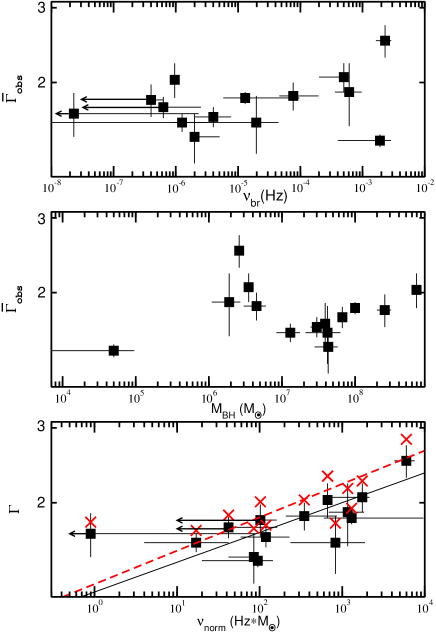
Figure 2: Top panel: The “$\bar{\Gamma}_{\rm obs}$ - break frequency” relation for the AGN in our sample. Middle panel: The “$\bar{\Gamma}_{\rm obs}$ - BH mass” relation for the same objects. Bottom panel: The AGN “mean spectral slope - normalised characteristic frequency” relation. Filled squares and crosses indicate the($\bar{\Gamma}_{\rm obs},\nu_{\rm norm}$) and the ($\bar{\Gamma}_{\rm 20\%},\nu_{\rm norm}$) data, respectively. The solid and dashed lines in the same panel indicate the best-fit power-law model to the ($\bar{\Gamma}_{\rm obs},\nu_{\rm norm}$) and ($\bar{\Gamma}_{\rm 20\%},\nu_{\rm norm}$) data, respectively.

Table 4: The Kendaull’s $\tau$ test results for the correlations plotted in Fig. 2.

	$\tau/$P${}_{\rm null}^{\rm a}$	$\tau^{\rm b}$/Pnull
$\bar{\Gamma}$ vs $\nu_{\rm bf}$	0.20/0.32	0.21/0.30
$\bar{\Gamma}$ vs BH mass	0.11/0.58	0.10/0.62
$\bar{\Gamma}$ vs $\nu_{\rm norm}$	0.53/$8.2\times 10^{-3}$	0.54/$7.3\times 10^{-3}$

^aP_null depends on both the size of the sample and the value of $\tau$.
^b Results in the case we use $\bar{\Gamma}_{\rm 20\%}$ instead of $\bar{\Gamma}_{\rm obs}$.

The Kendall’s $\tau$ results imply that only the “mean spectral slope vs $\nu_{\rm norm}$” correlation is strong (i.e $\tau>0.5$) and significant. This is true irrespective of whether we use $\bar{\Gamma}_{\rm 20\%}$ or $\bar{\Gamma}_{\rm obs}$. The correlation remains significant even if we omit Ark 564 (i.e. the source with the softest spectrum and the highest characteristic frequency): $\tau=0.45$, P${}_{\rm null}=0.03$ for the $\bar{\Gamma}_{\rm 20\%}$–$\nu_{\rm norm}$ relation, and $\tau=0.46$, P${}_{\rm null}=0.03$ when we use $\bar{\Gamma}_{\rm obs}$ instead of $\bar{\Gamma}_{\rm 20\%}$. We therefore conclude that, although the mean spectral slope does not correlate significantly either with power spectrum break frequency or with the BH mass, it does correlate positively with the break frequency when normalised to the BH mass of each object.

To investigate whether a straight line or a power law model fits best the AGN spectral-timing relation, we considered the 10 AGN that have well measured PSD breaks and we fitted their “average spectral slope - normalised frequency” data with a straight line in both the linear and log-log space, taking into account the errors on both the $\nu_{\rm norm}$ and $\bar{\Gamma}_{\rm obs}$ (or ${\Gamma}_{20\%}$) values. We found that the power-law model (i.e. a straight line in the log-log space) describes better the observed spectral-timing relation. For example, the linear model fit to the ($\bar{\Gamma}_{20\%}$, $\nu_{\rm norm}$) data resulted in a $\chi^{2}$ value of 25.1 for 8 degrees of freedom (dof). A linear model to the logarithm of the same data set resulted in 17.6 for 8 dof. To quantify if this change in $\chi^{2}$ is significant, we computed the “ratio of likelihoods”, $L_{1}/L_{2}$ (Mushotzky 1982). It is defined as $L_{1}/L_{2}$=exp$[(\chi^{2}_{2}-\chi^{2}_{1})/2]=$exp$(\Delta\chi^{2}/2)$, where $\chi^{2}_{1}$ and $\chi^{2}_{2}$ are the chisquare for the line fits in the logarithmic and linear spaces, respectively. We found that $L_{1}/L_{2}=42.5$. This result suggests that a power law is $\sim 40-45$ times more likely, than a straight line, to be the “correct” model for the spectral-timing data plotted in the bottom panel of Fig. 2.

To derive the best-fit power law parameter values, we used the “ordinary least squares bisector” method of Isobe et al. (1990) to fit the [log($\bar{\Gamma}_{\rm obs})$, log($\nu_{\rm norm}$)] data with a straight line of the form log($\bar{\Gamma}_{\rm obs})=a+b$log($\nu_{\rm norm}$). The best-fit parameter values are $a=0.09\pm 0.05$ and $b=0.070\pm 0.015$ (the best-fit model is indicated by the solid line in the bottom panel of Fig. 2). The dashed line in Fig. 2 indicates the best-fit straight line model to the [log$(\bar{\Gamma}_{\rm 20\%})$,log($\nu_{\rm norm}$)] data. The best-fit parameter values in this case are $a=0.11\pm 0.06$ and $b=0.079\pm 0.019$. In other words, a power-law model of the form $\bar{\Gamma}_{\rm obs}=1.23(\pm 0.14)\nu^{0.07\pm 0.015}_{\rm norm}$ fits well the ($\bar{\Gamma}_{\rm obs},\nu_{\rm norm}$) data, while in the case of the ($\bar{\Gamma}_{\rm 20\%},\nu_{\rm norm}$) data the best-fit power-law model is $\bar{\Gamma}_{\rm 20\%}=1.3(\pm 0.2)\nu^{0.079\pm 0.019}_{\rm norm}$. We note that although the best-fit slopes are small, they are significantly different than zero. The best-fit parameter values are consistent within the errors and their weighted mean value is $\bar{a}=0.10\pm 0.04$ and $\bar{b}=0.073\pm 0.012$. We therefore conclude that the spectral-timing relation in AGN is well parametrised by a power-law model of the form: $\Gamma_{\rm AGN}=1.26(\pm 0.12)\nu^{0.073\pm 0.012}_{\rm norm}$.

According to M06, the PSD break frequency depends on both the BH mass and accretion rate approximately as follows: $\nu_{\rm bf}\propto\dot{m}_{\rm E}/$M_BH. Consequently, $\nu_{\rm norm}$ should depend on $\dot{m}_{\rm E}$ only. Given this observational result, the $\bar{\Gamma}_{\rm AGN}\propto\nu_{\rm norm}^{0.07}$ relation we found can be translated to a $\bar{\Gamma}_{\rm AGN}\propto\dot{\rm m}_{\rm E}^{0.07}$ relation. In other words, our results suggest that the mean spectral slope in AGN correlates positively with $\dot{\rm m}_{\rm E}$: objects with higher accretion rate should also have steeper spectra (on average).

In the case of Comptonisation models, where thermal electrons in a corona above the disc upscatter soft photons emitted by the disc of temperature T_s, the produced X–rays have a power-law spectrum. When a soft photon of initial energy $\epsilon_{s}$ is Compton scattered in the corona, it acquires an energy $A\epsilon_{s}$, on average, where $A$ is the Compton amplification factor defined as $A=(L_{\rm diss}+L_{\rm s})/L_{\rm s}$ ($L_{\rm diss}$ and $L_{\rm s}$ are the power used to heat the corona and the intercepted soft luminosity, respectively). The produced X–rays have a power-law spectrum whose slope, $\Gamma$, depends on the temperature and optical depth of the corona. In general, one expects that when $L_{\rm s}$ increases, the corona cooling will be more efficient. Consequently, its temperature should decrease and the resulting X–ray spectrum will be steeper (i.e. $\Gamma$ will increase).

Using the numerical Comptonisation code of Coppi (1999; eqpair in XSPEC),which is applicable in the case of a soft photon source located in the centre of a static, isothermal spherical corona, Beloborodov (1999) derives a relationship between $\Gamma$ and $L_{s}/L_{diss}$ for different disc temperatures, Ts. For $T_{s}\sim$ few $\times 10^{4}K$, which is applicable in AGN, he finds that $\Gamma_{\rm AGN}\sim 2.3(L_{s}/L_{diss})^{0.1}$. For low mass black holes like Cyg X-1, where $T_{s}\sim$few $\times 10^{6}K$, $\Gamma_{\rm GBHs}\sim 2.3(L_{s}/L_{diss})^{0.17}$. In the case of a non-static, outflowing corona, Malzac, Beloborodov & Poutanen (2001) found similar results: $\Gamma_{\rm AGN}\sim 2.2(L_{s}/L_{diss})^{0.07}$ and $\Gamma_{\rm GBHs}\sim 2.2(L_{s}/L_{diss})^{0.13}$.

We found that $\Gamma_{\rm AGN}\propto\nu_{\rm norm}^{\sim 0.07}$ which, when combined with the $\nu_{\rm norm}\propto\dot{\rm m}_{\rm E}$ result of M06, implies that $\Gamma_{\rm AGN}\propto\dot{\rm m}_{\rm E}^{\sim 0.07}$. Consequently, thermal Comptonisation model predictions, i.e $\Gamma\propto(L_{s}/L_{diss})^{0.07}$ ^{or 0.10}, are consistent with our results, i.e $\Gamma_{\rm AGN}\propto\dot{\rm m}_{\rm E}^{\sim 0.07}$, but only if $L_{\rm s}/L_{\rm diss}\propto\dot{\rm m}_{\rm E}$.

5 Comparison with Cyg X-1

To compare the spectral-timing behaviour of AGN with that of Galactic black hole X-ray binary systems, we considered the extensive spectral and timing observations of the best studied GBH, Cyg X-1. To maximise the spectral-timing range, we considered all available information, covering “hard” state observations (from P03 and A06) and “soft” and “intermediate” states (from A06).

It is important that a consistent measure of characteristic break-frequency is used for all the Cyg X-1 and AGN data. In the soft state the PSD of Cyg X-1 is well described by a power-law with only one “bend”, with slope $\sim-1$ at low frequencies and $\sim-2$ at high frequencies. This shape is sometimes also parametrised as a power-law of slope -1 with an exponential cut-off (model 5 of A06). This shape also fits well the PSDs of almost all AGN that have been studied so far (except for Akn564, for which a double Lorentzian model fits best, M^cHardy et al. 2007). For the soft state PSDs of Cyg X-1 therefore, we considered from model 5 of A06, the best-fit “turnover” or “bend” frequency at which the PSD slope bends from $-1$ to $-2$.

In the hard state, the PSD of GBHs such as Cyg X-1 can be fitted either as a doubly bending power-law of slope 0 at the lowest frequencies, slope $-1$ at intermediate frequencies, and slope   $-2$ at the highest frequencies or, where the signal-to-noise ratio is higher, as the sum of a number of Lorentzian-shaped components. Both P03 and A06 have opted for the second option, in modeling the Cyg X-1 PSD in the hard and intermediate state. To include therefore the hard state Cyg X-1 PSD observations, we must use the Lorentzian which, in the bending power-law parametrization, is closest to the frequency at which the slopes change from $-1$ to $-2$. In the observations of P03, that Lorentzian is referred to as $\nu_{2}$, and has an average frequency around 2 Hz. In the analysis of A06 (and also of Axelsson, Borgonovo and Larsson, 2005), the hard and intermediate state PSD is parametrised by the sum of two Lorentzians but also with the addition of a weak cut-off power-law. The Lorentzian with the higher frequency corresponds to $\nu_{2}$ of P03 and so we used the frequency of that Lorentzian here.

In order to measure $\Gamma_{\rm obs}$, P03 fit their spectra with a “power-law + multi-temperature disc-black body + reflection” model from which the $\Gamma_{\rm obs}$ of the power-law can be taken. A06 list (20-9)/(4-2) keV hardness ratios (HR). We have used the empirical relationship between $\Gamma$ and HR of Axelsson et al. (2005) to convert HR into $\Gamma_{\rm obs}$.

The resulting Cyg X-1 data are shown in Fig.3. Open and filled circles indicate the ($\Gamma_{\rm obs},\nu_{2}$) data for Cyg X-1 where $\nu_{2}$ is the centroid frequency of the “second” Lorentzian in the P03 and A06 model fits to the Cyg X-1 PSD, respectively. These data define the Cyg X-1 spectral-timing relation in its hard state. Crosses indicate the ($\Gamma_{\rm obs},\nu_{c}$) data for Cyg X-1, where $\nu_{c}$ is the “bend” frequency of the “bending” power-law model which fits best the Cyg X-1 PSD in its soft state, according to A06 (their model 5). To convert the observed frequencies (both $\nu_{2}$ and $\nu_{c}$) to $\nu_{\rm norm}$ we assumed a black hole mass of 15 M_⊙, intermediate between the two published estimates of 10 M_⊙ (Herrero et al. 1995) and 20 M_⊙ (Ziolkowski 2005). We can see that the Cyg X-1 hard and soft state data form a smooth continuous distribution in the spectral-timing plane shown in Fig. 3.

Filled squares in the top and bottom panels of Fig. 3 indicate the “spectral slope – characteristic frequency” relation for the AGN in our sample, when we use the $\bar{\Gamma}_{\rm obs}$ and $\bar{\Gamma}_{20\%}$ values, respectively. Although in both Cyg X-1 and AGN the characteristic frequencies increase as the energy spectrum steepens, Fig. 3 shows clearly that the respective “$\Gamma-\nu_{\rm norm}$” relations are not the same.

This difference can be explained by the fact that the accretion disc is hotter in Cyg X-1 than in AGN. So, for example, in the case of an outflowing corona, as stated in Section 4.3, $\Gamma\propto(L_{s}/L_{diss})^{0.07}$ in AGN but $\Gamma\propto(L_{s}/L_{diss})^{0.13}$ in Cyg X-1. If $(L_{\rm s}/L_{\rm diss})\propto\dot{\rm m}_{\rm E}$, both in AGN and Cyg X-1, then we expect that $\Gamma_{\rm AGN}\propto\dot{\rm m}_{\rm E}^{0.07}$ and $\Gamma_{\rm CygX-1}\propto\dot{\rm m}_{\rm E}^{0.13}$. Using the $\nu_{\rm norm}\propto\dot{\rm m}_{\rm E}$ relation of M06, these relations can be written as follows: $\Gamma_{\rm AGN}\propto\nu_{\rm norm}^{0.07}$ and $\Gamma_{\rm CygX-1}\propto\nu_{\rm norm}^{0.13}$. As a result, in the case when $\Gamma_{\rm CygX-1}\approx\Gamma_{\rm AGN}$, we should expect that $\nu_{\rm norm,AGN}^{0.07}\sim\nu_{\rm norm,CygX-1}^{0.13}$, i.e. $\nu_{\rm norm,CygX-1}\sim\nu_{\rm norm,AGN}^{0.55}$ (in the case of a static corona, we expect a similar relation, i.e. $\nu_{\rm norm,CygX-1}\sim\nu_{\rm norm,AGN}^{0.6}$). Open squares in both panels of Fig. 2 indicate the AGN data when we transform $\nu_{\rm norm,AGN}$ to $\nu_{\rm norm,AGN}^{0.55}$. The agreement now between the Cyg X-1 and AGN “spectral slope - characteristic frequency” relation is good (a more detailed derivation of the relation between $\nu_{\rm norm,AGN}$ and $\nu_{\rm norm,CygX-1}$ in the case of thermal Comptonisation models is presented in Section 6.2).

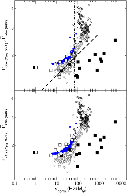
Figure 3: (Both panels) Filled and open circles indicate the spectral-timing data for Cyg X-1 in its hard state, using data from P03 and A06, respectively. Crosses indicate the spectral-timing data for Cyg X-1 in its soft state using data from A06. Filled squares indicate the “mean spectral slope - normalised characteristic frequency” data for the AGN in our sample, when we consider the $\bar{\Gamma}_{\rm obs}$ and the $\bar{\Gamma}_{20\%}$ values listed in Table 3 (top and bottom panels, respectively). Open squares indicate the same AGN data when $\nu_{\rm norm,AGN}$ are shifted to $\nu_{\rm norm,AGN}^{0.55}$ (see text for details).

6 Discussion and conclusions

We have used 7795 RXTE observations of 11 AGN, obtained over a period of $\sim 7-11$ years, to extract their 3–20 keV spectra. We fitted them with a simple “power-law + Gaussian line” model, and we used the best-fit slopes to construct their sample distribution function. We used the median of the distributions, and the mean of the best-fit slopes which are above the 80th percentile of the distributions, to estimate the mean spectral slope of the objects (the latter estimate is more appropriate in the case when the energy spectra of the sources are significantly affected by absorption and/or reflection effects). We also used results from literature to estimate the average spectral slope of three more objects. The fourteen AGN that we consider in this work are nearby, X–ray bright objects, whose X–ray light curves have been studied in the past. Their PSDs have been accurately estimated, and characteristic “break frequencies” have been detected in them.

When we combine the mean spectral slope estimates with the $\nu_{\rm br}$ estimates listed in UM05, we find that: objects with steeper mean energy spectra have shorter characteristic time scales as well. This is the first time that such a “spectral – timing” correlation is detected in AGN. The results we reported in Section 4.3 suggest that this spectral-timing relation in AGN can be parametrised as follows: $\Gamma\approx 1.3\nu_{\rm norm}^{0.07}$.

6.1 The spectral-timing correlation in AGN

The easiest way to explain this correlation is to assume that, for an AGN with a given BH mass, the accretion rate determines both the PSD characteristic frequencies (this has already been shown by M06) and their energy spectral shape as well: the higher the accretion rate, the steeper the mean energy spectrum will be. Such a positive $\Gamma-\dot{\rm m}_{\rm E}$ relation in AGN has already been suggested/shown in the past (e.g. Porquet et al. 2004; Bian 2005; Shemmer et al. 2006; Saez et al. 2008). A positive $\Gamma-\dot{\rm m}_{\rm E}$ relation has also been detected recently in 7 GBHs by Wu & Gu (2008), when they accrete at a rate higher than $\sim 1\%$ of the Eddington limit. Our results are consistent with the results reported in these papers.

Using the above results and the M06 results, we calculate that $\nu_{\rm norm}($Hz$\times$M${}_{\odot})\approx 3000\dot{\rm m}_{\rm E}$. When we replace $\nu_{\rm norm}$ in the relation of $\Gamma\approx 1.3\nu_{\rm norm}^{0.07}$ we found in this work, we find that: $\Gamma\approx 2.3\dot{\rm m}_{\rm E}^{0.07}$. This formula between spectral slope and accretion rate could be helpful in deriving a rough estimate for the accretion rate of the distant AGN that are detected in deep X-ray surveys, assuming that their variability properties are similar to the properties of nearby AGN (this is supported by recent studies, see e.g. Papadakis et al. 2008).

In the context of thermal Comptonisation models, $\dot{\rm m}_{\rm E}$ can affect the spectral slope $\Gamma$ as it controls the strength of the soft disc photons, hence the cooling of the thermal plasma in the X-ray emitting corona. The greater the cooling by seed photons incident on the plasma, the softer the resulting X-ray power-law spectra are. Indeed, we found that Comptonisation models are consistent with the $\Gamma-\dot{\rm m}_{\rm E}$ relation that our results imply, but only if $L_{\rm s}/L_{\rm diss}\propto\dot{\rm m}_{\rm E}$.

6.2 The comparison with Cyg X-1

Both P03 and A06 have used data from RXTE observations that lasted for $\sim 1-2$ ks, and were performed every $\sim 5-10$ days over a period of many years. If “time scales” scale with BH mass in accreting objects, then $1-2$ ksec in Cyg X-1 should correspond to a period of at least $\sim 3-6$ years in objects with M${}_{\rm BH}>10^{6}$ times the mass of the black hole in Cyg X-1 (like most AGN in our sample). This suggests that each one of the AGN points in Fig. 3 corresponds to just one of the Cyg X-1 points plotted in the same figure. We found that the AGN and Cyg X-1 “$\Gamma-\nu_{\rm norm}$” relations are similar but not the same. In Section 5 we discussed briefly some implications of this result. In the paragraphs below we discuss the implications of our results in more detail.

The main aim of the discussion below is to investigate the constrains that the AGN spectral-timing relation, and its comparison with the similar relation in Cyg X-1, impose on thermal Comptonisation models, based on the particular assumption that both the spectral and timing properties of accreting systems are driven by accretion rates variations. We point out that other interpretations are also possible; see for example Kylafis et al. (2008) for an alternative explanation of the Cyg X-1 spectral-timing relation, which does not assume that X–rays are produced by thermal Comptonisation. We also point out that, given the small number of objects in our sample, and the unavoidable uncertainty in the derived parameters of the AGN spectral-timing relation, the values of the various parameters in the equations below are somehow uncertain.

As we showed in Section 6.1, the AGN spectral-timing relation and the M06 results imply that $\Gamma_{\rm AGN}\approx 2.3\dot{m}_{\rm E}^{0.07}$. If X–rays in AGN are produced by thermal Comptonisation, we expect that $\Gamma_{\rm AGN}=2.2(L_{\rm s}/L_{\rm diss})^{0.07}$. Therefore, the observations [i.e. $\Gamma_{\rm AGN}\approx 2.3\dot{m}_{\rm E}^{0.07}$] are consistent with the thermal Comptonisation model predictions [$\Gamma_{\rm AGN}=2.2(L_{\rm s}/L_{\rm diss})^{0.07}$], only if

$$(L_{\rm s}/L_{\rm diss})\approx 2\dot{m}_{\rm E}.$$ (1)

An obvious implication of this result is that, if a certain fraction, say $f_{\rm s}$, of the total accretion power, $P_{\rm tot}$ $(=\eta\dot{m}_{\rm E}c^{2},$ where $\eta$ is the efficiency of the accretion process), is converted to disc luminosity (i.e. $L_{\rm s}=f_{\rm s}P_{\rm tot}$), while $L_{\rm diss}=f_{\rm diss}P_{\rm tot}$, then the ratio $(f_{\rm s}/f_{\rm diss})$ should not remain constant for a given object, but should rather increase with increasing accretion rate.

Suppose that X–rays from Cyg X-1 in its low/hard state (LH) are also produced by thermal Comptonisation. In this case, thermal Comptonisation models predict that $\Gamma_{\rm CygX-1}=2.2(L_{\rm s}/L_{\rm diss})^{0.13}$, or

$$\Gamma_{\rm CygX-1}\approx 2.4\dot{m}_{\rm E}^{0.13},$$ (2)

if we accept that equation (1) holds in this case as well. According to Körding et al. (2007), the normalisation of the $\nu_{\rm norm}$ vs $\dot{m}_{\rm E}$ relation for the hard-state GBHs is $\sim 8$ times smaller than the normalisation in the case of the AGN in our sample. So, if $\nu_{\rm norm,CygX-1/LS}\approx 375\dot{m}_{\rm E}$, as opposed to $\nu_{\rm norm,AGN}\approx 3000\dot{m}_{\rm E}$, then $\dot{m}_{\rm E}\approx 3\times 10^{-3}\nu_{\rm norm,CygX-1/LS}.$ We can now substitute $\dot{m}_{\rm E}$ in equation (2) to determine the $\Gamma-\nu_{\rm norm}$ relation for Cyg X-1 in LH state:

$$\Gamma_{\rm CygX-1/LS}\approx 1.1\nu_{\rm norm}^{0.13}.$$ (3)

The dashed line in the top panel of Fig. 3 indicates this relation. The agreement between the predicted $\Gamma-\nu_{\rm norm}$ relation and the Cyg X-1 data is rather good up to $\nu_{\rm norm}\sim 70$. The discussion so far suggests the following picture:

a) X-rays from the AGN we studied are produced by thermal Comptonisation. The $\Gamma-\nu_{\rm norm}$ relation we observe is consistent with the predictions of thermal Comptonisation models but only if the $(L_{\rm s}/L_{\rm diss})$ ratio, and hence the $(f_{\rm s}/f_{\rm diss})$ ratio as well, increase proportionally with accretion rate.

b) X-rays in Cyg X-1 are also produced by thermal Comptonisation. Taking into account the fact that the normalisation of the $\nu_{\rm norm}-\dot{m}_{\rm E}$ relation is $\sim 8$ times smaller in Cyg X-1 than in the AGN in our sample (Körding et al. 2007), the predicted $\Gamma-\nu_{\rm norm}$ relation agrees well with the Cyg X-1 data up to $\nu_{\rm norm}\approx 70$.

c) In the case when $\Gamma_{\rm AGN}=\Gamma_{\rm CygX-1}$, we expect that ($L_{\rm s}/L_{\rm diss})_{\rm CygX-1}^{0.13}=(L_{\rm s}/L_{\rm diss})_{\rm AGN}^{0.07}$, and $\dot{m}_{\rm AGN,E}^{0.07}=\dot{m}_{\rm CygX-1,E}^{0.13}$ (using equation 1). Consequently, $\dot{m}_{\rm E,AGN}=\dot{m}_{\rm E,CygX-1}^{1.9}$ and, since $\dot{m}_{\rm E}<1$, AGN should operate on a lower accretion rate than Cyg X-1 when the spectral slope is the same in both systems. Furthermore, since $\Gamma_{\rm AGN}\approx 1.3\nu_{\rm norm,AGN}^{0.07}$ and $\Gamma_{\rm CygX-1}\approx 1.1\nu_{\rm norm,CygX-1}^{0.13}$ (when $\Gamma\leavevmode\nobreak\ \raise 2.15277pt\hbox{$<$}\kern-8.00003pt\lower 2.84526pt\hbox{$\sim$}\leavevmode\nobreak\ 2.1-2.2$), then $\Gamma_{\rm AGN}=\Gamma_{\rm CygX-1}$ implies that $1.3\nu_{\rm norm,AGN}^{0.07}=1.1\nu_{\rm norm,CygX-1}^{0.13}$, and $\nu_{\rm norm,CygX-1}\approx 3.5\nu_{\rm norm,AGN}^{0.55}$. Therefore, when the spectral slope is the same (and less than $\sim 2.1-2.2$) in AGN and Cyg X-1, the former should operate at a lower accretion rate but their characteristic time scales should be shorter than those in Cyg X-1 (when normalised to the respective BH mass), because the normalisation of the AGN $\dot{m}-\nu_{\rm norm}$ relation is significantly larger than the normalisation of the respective Cyg X-1 relation in LH state.

The vertical dot-dashed line in the top panel of Fig. 3 indicates the value $\nu_{\rm norm}=70$. For Cyg X-1, this normalised frequency corresponds to $\nu_{1}=1$ Hz and $\nu_{2}=5$ Hz for the centroid frequency of the low and higher frequency Lorentzians, respectively. As $\nu_{\rm norm}$ (i.e. the accretion rate) increases even more, then i) the ratio $\nu_{1}/\nu_{2}$ increases as well (see Fig. 2 in A06), ii) the contribution of the Lorentzians to the root mean square variability amplitude decreases, and iii) the “bending” power-law component in the PSD appears and its contribution to the source variability amplitude increases (see Fig. 7 in A06), i.e. the Cyg X-1 power spectrum changes from a hard to a soft-state shape. At $\nu_{\rm norm}\approx 70$, the average observed spectral slope of Cyg X-1 is $\sim 2.1$ (see Fig. 3), while at higher frequencies the spectral slope is steeper. Consequently, the region defined by $\Gamma<2.1$ and $\nu_{\rm norm}<70$ corresponds to the “hard state region” for Cyg X-1 in the “spectral-timing plane” shown in Fig. 3.

The discrepancy between the predicted spectral-timing relation and the Cyg X-1 data when $\Gamma\leavevmode\nobreak\ \raise 2.15277pt\hbox{$>$}\kern-8.00003pt\lower 2.84526pt\hbox{$\sim$}\leavevmode\nobreak\ 2.1$ and $\nu_{\rm norm}\leavevmode\nobreak\ \raise 2.15277pt\hbox{$>$}\kern-8.00003pt\lower 2.84526pt\hbox{$\sim$}\leavevmode\nobreak\ 70$ cannot be explained by the fact that the normalisation of the $\nu_{\rm norm}-\dot{m}_{\rm E}$ relation increases by a factor of $\sim 8$ in the high/soft state. If that were the case, the spectral-timing relation in this state should be similar to the one defined by equation (3), but with a smaller normalisation (opposite to what we observe).

One possibility is that the $(L_{\rm s}/L_{\rm diss})-\dot{m}_{E}$ relation (equation 1) changes in the high/soft state. However, in this case we would have to accept that the X–ray source does not operate in the same way in AGN and Cyg X-1: when $\nu_{\rm norm}>70$, both Cyg X-1 and the AGN in our sample follow the same $\nu_{\rm norm}-\dot{m}_{\rm E}$ relation (M06, Körding et al. 2007). Therefore, as long as $\nu_{\rm norm}>70$, a given $\nu_{\rm norm}$ value implies the same accretion rate in both systems. The fact that the AGN spectral-timing relation is valid up to $\nu_{\rm norm}\approx 1000$ should then imply that, for the same accretion rate, the “$(L_{\rm s}/L_{\rm diss})-$ accretion rate” relation is different in AGN and Cyg X-1.

In Cyg X-1, $\Gamma\approx 2.1$ implies that $2.2(L_{\rm s}/L_{\rm diss})^{0.13}\approx 2.1$, and hence $(L_{\rm s}/L_{\rm diss})\approx 0.7$. Another possible explanation then for the discrepancy between the Cyg X-1 data and the predicted spectral-timing relation above $\nu_{\rm norm}=70$ is the following: equation (1) holds until $(L_{\rm s}/L_{\rm diss})\approx 0.7$, at which point the hot corona is significantly cooled down, and the thermal X–ray emission component is weak. It is possible then that at high accretion rates a separate, possibly non-thermal, X–ray component emerges, and dominates the X-ray emission in the soft state. If that is the case, the $\Gamma-L_{\rm s}/L_{\rm diss}$ relation we have assumed above is not valid, hence the predicted spectral-timing relation does not fit the data any more.

Even if the picture drawn above is correct, there are important issues regarding the relation between AGN and GBH states which still remain unresolved. In particular, the answer to the question whether the AGN in our sample are “soft” or “hard” state systems is far from clear. There are indications that they are analogous to Cyg X-1 in its soft state. For example, the radio emission in Cyg X-1 in its LH state is enhanced. On the other hand, Panessa et al. (2007) have shown that, for the same $L_{\rm X}/L_{\rm E}$ ratio, the radio luminosity of Seyfert galaxies is $\sim 8-10$ times lower than the radio luminosity of hard-state GBHs, even when the BH mass difference is properly taken into account (7 of the objects in our sample are also included in their sample). Furthermore, the AGN in our sample follow the soft-state “characteristic time scale – accretion relation” in GBHs, and a “bending” power-law is the dominant component in the power spectrum of those objects with good enough light curves to accurately study their PSD (e.g. NGC 4051, M^cHardy et al. 2004; NGC 3227 and NGC 5506, UM05; MCG 6-30-15, M^cHardy et al. 2005; and perhaps NGC 3783, Summons et al. 2007), implying a soft-state like PSD in these objects. High quality light curves for low accretion rate AGN are necessary to investigate whether any AGN with hard-state like power spectra exist or not.

However, although the radio emission strength and the timing properties of many objects in our sample are soft-state like, their spectral properties are not, as the average spectral slope is smaller than $2.1$ in most cases. If indeed the spectral hard-to-soft state transition corresponds to $(L_{\rm s}/L_{\rm diss})\sim 0.7$, at which point the thermal corona emission is weak, and a different component dominates the X–ray emission, then we should expect this transition to happen when $\Gamma\leavevmode\nobreak\ \raise 2.15277pt\hbox{$>$}\kern-8.00003pt\lower 2.84526pt\hbox{$\sim$}\leavevmode\nobreak\ 2.15$ in AGN. Given the AGN $\Gamma-\nu_{\rm norm}$ relation, this slope corresponds to $\nu_{\rm norm}\approx 2500$. At even higher normalised frequencies, we should then expect the AGN spectral-timing relation to break (like in Cyg X-1 at $\nu_{\rm norm}\approx 70$). Obviously, more data are necessary to confirm that this is indeed the case in AGN.

The data so far suggest that while in AGN the timing properties transition from hard-to-soft state happens at least as low as $\nu_{\rm norm}\approx 100$, the spectral properties transition should happen at much higher accretion rates. This is opposite to what we observe in Cyg X-1, where both the spectral and timing properties change from the hard to soft state, at the same accretion rate (indicated by the value $\nu_{\rm norm}\approx 70)$. Perhaps the timing properties in accreting objects are determined by accretion disc variations only, and the hard-to-soft state transition materialises at a certain accretion rate, irrespective of whether the soft disc luminosity is strong enough for $(L_{\rm s}/L_{\rm diss})>0.7$, i.e. strong enough to cool down the hot corona. In this case, we would expect the AGN hard-to-soft timing properties transition to appear at $\nu_{\rm norm}\approx 70$ as well. Due to the cooler disc temperature though, the AGN spectral soft-to-hard state transition happens at higher accretion rates (i.e. at a higher $\nu_{\rm norm}$ value in the spectral-timing plane of Fig. 3). Further progress in understanding the relation between AGN and GBHs can be made when we know how the accretion rate determines the characteristic frequency in accreting compact objects (assuming that it is just the accretion rate that determines $\nu_{\rm norm}$ in these systems).

- (1) Arnaud, K.A. 1996, Astronomical Data Analysis Software and Systems V, eds. Jacoby G. & Barnes J., ASP Conf. Series, 101, 17
- (2) Axelsson, M., Borgonovo, L., & Larsson, S. 2006, A&A, 452, 975 (A06)
- (3) Axelsson, M., Borgonovo, L., & Larsson, S. 2005, A&A, 438, 999
- (4) Beckmann, V., Shrader, C. R., Gehrels, N., et. al. 2005, ApJ, 634, 939
- (5) Beloborodov, A.M. 1999, in J. Poutanen and R. Svensson, Editors, “High Energy Processes in Accreting Black Holes”, Astron. Soc. Pac., San Francisco (1999), 295
- (6) Bianchi, S., Balestra, I., Matt, G., Guainazzi, M., & Perola, G. C. 2003, A&A, 402, 141B
- (7) Bian, W. 2005, ChJAS, 5, 289
- (8) Botte, V., Ciroi, S., Rafanelli, P., & Di Mille, F. 2004, AJ, 127, 3168
- (9) Coppi, P. S. 1999, in J. Poutanen and R. Svensson, Editors, “High Energy Processes in Accreting Black Holes”, Astron. Soc. Pac., San Francisco (1999), 375
- (10) de Rosa, A., Piro, L., Perola, G. C., et al. 2007, A&A, 463, 903
- (11) Fiore, F., Pellegrini, S., Matt, G., et al. 2001, ApJ, 556, 150
- (12) Fruscione, A., Greenhill, L. J., Filippenko, A. V., Moran, J. M., Herrnstein, J. R., & Galle, E. 2005, ApJ, 624, 103
- (13) Herrero, A., Kudritzki, R. P., Gabler, R., Vilchez, J. M., & Gabler, A. 1995, A&A, 297, 556
- (14) Herrnstein, J. R., Moran, J. M., Greenhill, L. J., et al. 1999, Nature, 400, 539
- (15) Jahoda, K., Swank, J. H., Giles, A. B., et al. 1996, Proc. SPIE, 2808, 59
- (16) Isobe, T., Feigelson, E. D., Akritas, M. G., & Babu, G. J. 1990, ApJ, 364, 104
- (17) Körding, E. G., Migliari, S., Fender, R., Belloni, T., Knigge, C., & McHardy, I., 2007, MNRAS, 380, 301
- (18) Kraemer, S.B., George, I.M., Crenshaw, D.M., et al. 2005, ApJ, 633, 693
- (19) Kylafis, N. D., Papadakis, I. E., Reig, P., Giannios, D. & Pooley, G. G. 2008, A&A, 489, 481
- (20) Lamer, G., Uttley, P., & McHardy, I. M. 2003, MNRAS, 342, 41
- (21) Lamer, G., Uttley, P., & McHardy, I. M. 2000, MNRAS, 319, 949
- (22) Malzac, J., Beloborodov, A. M., & Poutanen, J. 2001, MNRAS, 326, 417
- (23) Markowitz, A., Edelson, R., Vaughan, S., et al. 2003, ApJ, 593, 96
- (24) McHardy, I. M., Papadakis, I. E., Uttley, P., Page, M. J., & Mason, K. O. 2004, MNRAS, 348, 783
- (25) McHardy, I.M., Gunn, K.F., Uttley, P., & Goad, M. 2005, MNRAS, 359, 1469
- (26) McHardy, I.M., Köerding, E., Knigge, C., Uttley, P., & Fender, R. P. 2006, Nature, 444, 730 (M06)
- (27) McHardy, I., Arevalo, P., Uttley, P., Papadakis, I. E., Summons, D., Brinkmann, W., & Page, M. J. 2007, MNRAS, 382, 985
- (28) Miller, L., Turner, T. J., & Reeves, J.N. 2008, A&A, 483, 437
- (29) Miniutti, G., Fabian, A.C., Anabuki, N., et al., 2007, PASJ, 59, 315
- (30) Mushotzky, R. F, 1982, ApJ, 256, 92
- (31) Nagar, N. M., Oliva, E., Marconi, A., & Maiolino, R. 2002, A&A, 391, 21L
- (32) Panessa, F., Barcons, X., Bassani, L., Cappi, M., Carrera, F.J., Ho, L.C., & Pellegrini, S. 2007, A&A, 467, 519
- (33) Papadakis, I. E., Brinkmann, W., Negoro, H., & Gliozzi, M. 2002, A&A, 382, L1
- (34) Papadakis, I. E., Reig, P., & Nandra, K. 2003, MNRAS, 344, 993
- (35) Papadakis, I. E. 2004, MNRAS, 348, 207
- (36) Papadakis, I.E., Chatzopoulos, E., Athanasiadis, D., Markowitz, A., & Georgantopoulos, I. 2008, A&A, 487, 475
- (37) Peterson, B. M., Ferrarese, L., Gilbert, K. M., et al. 2004, ApJ, 613, 682
- (38) Ponti, G., Miniutti, G., Cappi, M., Maraschi, L., Fabian, A.C., & Iwasawa, K. 2006, MNRAS, 368, 903
- (39) Porquet, D., Reeves, J. N., O’Brien, P., & Brinkmann, W. 2004, A&A, 422, 85
- (40) Pottschmidt, K., Wilms, J., Nowak, M. A., et al. 2003, A&A, 407, 1039 (P03)
- (41) Reeves, J.N., Nandra, K., George, I.M., Pounds, K.A., Turner, T.J., & Yaqoob, T. 2004, ApJ, 602, 648
- (42) Saez, C., Chartas, G., Brandt, W. N., Lehmer, B. D., Bauer, F. E., Dai, X., & Garmire, G. P. 2008, AJ, 135, 1505
- (43) Shaposhnikov, N., & Titarchuk, L. 2006, ApJ, 643, 1098
- (44) Shemmer, O., Brandt, W.N., Netzer, H., Maiolino, R., & Kaspi, S. 2006, ApJ, 646, L29
- (45) Shih, D. C., Iwasawa, K., & Fabian, A. C. 2003, MNRAS, 341, 973
- (46) Taylor, R. D., Uttley, P., & McHardy, I. M. 2003, MNRAS, 342, L31
- (47) Turner, T.J., Kraemer, S.B., George, I.M., Reeves, J.N., & Bottorff, M.C. 2005, ApJ, 618, 155
- (48) Summons, D. P., Arevalo, P., McHardy, I. M., Uttley, P., & Bhaskar, A. 2007, MNRAS, 378, 649
- (49) Turner, T. J., Miller, L., Reeves, J. N., & Kraemer, S. B. 2007, A&A, 475, 121
- (50) Uttley, P., McHardy, I. M., & Papadakis, I. E. 2002, MNRAS, 332, 231
- (51) Uttley, P., Taylor, R. D., & McHardy, I. M. 2004, MNRAS, 347, 1345
- (52) Uttley, P., & McHardy, I. M. 2005, MNRAS, 363, 586 (UM05)
- (53) Vaughan, S., & Fabian, A. C. 2003, MNRAS, 341, 496
- (54) Vaughan, S., Iwasawa, K., Fabian, A.C., & Hayashida, K. 2005, MNRAS, 356, 524
- (55) Woo, J.-H., & Urry, C. M. 2002, ApJ, 579, 530
- (56) Wu, Q., & Gu, M. 2008, ApJ, 682, 212
- (57) Ziolkowski, J. 2005, MNRAS, 358, 851