Technical report on a long-wave unstable thin film equation with convection

Abstract

In this technical report, we consider a nonlinear 4th-order degenerate parabolic partial differential equation that arises in modelling the dynamics of an incompressible thin liquid film on the outer surface of a rotating horizontal cylinder in the presence of gravity. The parameters involved determine a rich variety of qualitatively different flows. Depending on the initial data and the parameter values, we prove the existence of nonnegative periodic weak solutions. In addition, we prove that these solutions and their gradients cannot grow any faster than linearly in time; there cannot be a finite-time blow-up. Finally, we present numerical simulations of solutions.

2000 MSC: 35K65, 35K35, 35Q35, 35G25, 35B40, 35B99, 35D05, 76A20

keywords: fourth-order degenerate parabolic equations, thin liquid films, convection, rimming flows, coating flows

1 Introduction

We consider the dynamics of a viscous incompressible fluid on the outer surface of a horizontal circular cylinder that is rotating around its axis in the presence of gravity, see Figure 1.

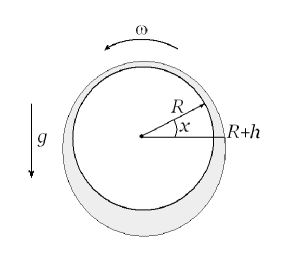
Figure 1: Liquid film on the outer surface of a rotating horizontal cylinder in the presence of gravity.

If the cylinder is fully coated there is only one free boundary: where the liquid meets the surrounding air. Otherwise, there is also a free boundary (or contact line) where the air and liquid meet the cylinder’s surface.

The motion of the liquid film is governed by four physical effects: viscosity, gravity, surface tension, and centrifugal forces. These are reflected in the parameters: $R$ — the radius of the cylinder, $\omega$ — its rate of rotation (assumed constant), $g$ — the acceleration due to gravity, $\nu$ — the kinematic viscosity, $\rho$ — the fluid’s density, and $\sigma$ — the surface tension.

These parameters yield three independent dimensionless numbers: the Reynolds number $\mbox{Re}=(R^{2}\omega)/\nu$, the Galileo number $\mbox{Ga}=g/(R\omega^{2})$ and the Weber number $\mbox{We}=(\rho R^{3}\omega^{2})/\sigma$.

We introduce the parameter $\epsilon=\bar{h}/R$, where $\bar{h}$ is the average thickness of the liquid. The following quantities are assumed to have finite, nonzero limits in the thin film ($\epsilon\to 0$) limit [27, 28, 2, 23]:

$$\kappa=\mbox{Re}\,\epsilon^{2},\quad\chi=\tfrac{\mbox{Re}}{\mbox{We}}\,\epsilon^{2},\quad\mbox{and}\quad\mu=\mbox{Ga}\,\mbox{Re}\,\epsilon^{2}.$$ (1.1)

This corresponds to a low rotation rate, for example.

One can model the flow using the full three-dimensional Navier-Stokes equations with free boundaries: for $\vec{u}(x,y,z,t)$ in the region $x\in[-\pi,\pi)$, $y\in\mathbb{R}^{1}$, and $z\in(0,h(x,y,t))$ where $x$ is the angular variable, $y$ is the axial variable, and $h(x,y,t)$ is the thickness of the fluid above the point $(x,y)$ on the surface of the cylinder at time $t$. This has been done by Pukhnachov [27] in which he considered the physical regime for which the ratio of the free-fall acceleration and the centripetal acceleration is small. There, he proved the existence and uniqueness of fully-coating steady states (no contact line is present). We know of no results for the affiliated initial value problem.

In this physical regime, if one also makes a longwave approximation (the thickness of the coating fluid is smaller than the radius of the cylinder) and if one further assumes that the rotation rate is low (or the viscosity is large) then the three-dimensional Navier-Stokes equations with free boundary can be approximated by a fourth-order degenerate partial differential equation (PDE) for the film thickness $h(x,y,t)$. This is done by averaging the fluid flow in the direction normal to the cylinder [27, 28]. If one further assumes that the flow is independent of the axial variable, $y$, then this results in a PDE in one dimension for $h(x,t)$.

In his pioneering 1977 article about syrup rings on a rotating roller, Moffatt neglected the effect of surface tension (i.e. $\mbox{We}^{-1}=0=\chi$), assumed the flow was uniform in the axial variable, and derived [23] the following model for the thin film thickness:

$$h_{t}+\left(h-\tfrac{\mu}{3}h^{3}\,\cos(x)\right)_{x}=0,$$ (1.2)

where $\mu$ is given in (1.1) and

$$x\in[-\pi,\pi],\quad t>0,\quad h\text{ is }2\pi\text{-periodic in }x.$$

Pukhnachov’s 1977 article [27] gives the first model that takes into account surface tension:

$$h_{t}+(h-\tfrac{\mu}{3}h^{3}\,\cos(x))_{x}+\tfrac{\chi}{3}\,\left(h^{3}\left(h_{x}+h_{xxx}\right)\right)_{x}=0$$ (1.3)

where $\mu$ and $\chi$ are given in (1.1) and

$$x\in[-\pi,\pi],\quad t>0,\quad h\text{ is }2\pi\text{-periodic in }x.$$

This model assumes a no-slip boundary condition at the liquid/solid interface. For a solution to (1.2) or (1.3) to be physically relevant, either $h$ is strictly positive (the cylinder is fully coated) or $h$ is nonnegative (the cylinder is wet in some region and dry in others).

Surprisingly little is understood about the initial value problem for (1.3). Bernis and Friedman [5] were the first to prove the existence of nonnegative weak solutions for nonnegative initial data for the related fourth-order nonlinear degenerate parabolic PDE

$$h_{t}+(f(h)\,h_{xxx})_{x}=0,$$ (1.4)

where $f(h)=|h|^{n}\,f_{0}(h),\quad f_{0}(h)>0,\quad n\geqslant 1$.

Unlike for second-order parabolic equations, there is no comparison principle for equation (1.4). Nonnegative initial data does not automatically yield a nonnegative solution; indeed it may not even be true for general fourth-order PDE (e.g. consider $h_{t}=-h_{xxxx}$). The degeneracy $f(h)$ in equation (1.4) is key in ensuring that nonnegative solutions exist. Also, unlike for second-order problems, it is possible that strictly positive initial data might yield a solution that is zero at certain moments in time, at certain locations in space.

Lower-order terms can be added to equation (1.4) to model additional physical effects. For example,

$$h_{t}+(f(h)\,h_{xxx})_{x}-(g(h)h_{x})_{x}=0$$ (1.5)

where $g(h)>0$ for $h\neq 0$. Equation (1.5) can model a thin liquid film on a horizontal surface with gravity acting towards the surface. If this surface is not horizontal then the dynamics can be modelled by

$$h_{t}+(h^{n}(a-b\,h_{x}+h_{xxx}))_{x}=0,\ \ a>0,\ \ b\geq 0$$ (1.6)

The constant $a$ in the first-order term vanishes as the surface becomes more and more horizontal. If the thin film of liquid is on a horizontal surface with gravity acting away from the surface then the thin film dynamics can be modelled by

$$h_{t}+(f(h)\,h_{xxx})_{x}+(g(h)h_{x})_{x}=0.$$ (1.7)

For a thorough review of the modelling of thin liquid films, see [13, 24, 26].

In equations (1.5) and (1.6) the second-order term is stabilizing: if one linearizes the equation about a constant, positive steady state then the presence of the second-order term increases how quickly perturbations decay in time. In equation (1.7), the second-order term is destabilizing: the linearized equation can have some long-wavelength perturbations that grow in time. For this reason, we refer to equation (1.7) as ‘‘long–wave unstable’’. The long–wave stable equations (1.5) and (1.6) have similar dynamics as equation (1.4) however the long-wave unstable equation (1.7) can have nontrivial exact solutions and can have finite–time blow–up ($h(x^{*},t)\uparrow\infty$ as $t\uparrow t^{*}<\infty$).

In all cases, the fourth-order term makes it harder to prove desirable properties such as: the short–time (or long–time) existence of nonnegative solutions given nonnegative initial data, compactly supported initial data yielding compactly supported solutions (finite speed of propagation), and uniqueness. Indeed, there are counterexamples to uniqueness of weak solutions [3]. Results about existence and long–time behavior for solutions of (1.5) can be found in [6]; analogous results for (1.6) are in [17]. See [8, 9] for results about existence, finite speed of propagation, and finite–time blow–up for equation (1.7).

In this paper we study the existence of weak solutions of the thin film equation

$$h_{t}+\left({|h|^{3}(a_{0}\,h_{xxx}+a_{1}h_{x}+a_{2}w^{\prime}(x))}\right)_{x}+a_{3}h_{x}=0$$ (1.8)

where $a_{1},\,a_{2},\,a_{3}$ are arbitrary constants, constant $a_{0}>0$, and $w(x)$ is periodic. Equation (1.3) is a special case of (1.8). The sign of $a_{1}$ determines whether equation (1.8) is long–wave unstable. Also, the coefficient of the convection term $a_{2}(w^{\prime}(x)|h|^{3})_{x}$ can depend on space and will change sign if $a_{2}w^{\prime}(x)\not\equiv 0$. The cubic nonlinearity $|h|^{3}$ in equation (1.8) arises naturally in models of thin liquid films with no-slip boundary conditions at the liquid/solid interface. Our methods generalize naturally to $f(h)=|h|^{n}$ for an interval of $n$ containing 3; we refer the reader to [3, 5, 7] for the types of results expected.

Given nonnegative initial data that satisfies some reasonable conditions, we prove long-time existence of nonnegative periodic generalized weak solutions to the initial value problem for equation (1.8). We start by using energy methods to prove short-time existence of a weak solution and find an explicit lower bound on the time of existence. A generalization and sharpening of the method used in [8] allows us to prove that the $H^{1}$ norm of the constructed solution can grow at most linearly in time, precluding the possibility of a finite–time blow–up. This $H^{1}$ control, combined with the explicit lower bound on the (short) time of existence, allows us to continue the weak solution in time, extending the short-time result to a long-time result.

If $a_{2}=0$ or $a_{3}=0$ in equation (1.8) then solutions will be uniformly bounded for all time. If $a_{2}\neq 0$ and $a_{3}\neq 0$, it is natural to ask if the nonlinear advection term could cause finite–time blow–up ($h(x^{*},t)\uparrow\infty$ as $t\uparrow t^{*}$ at some point $x^{*}$). Such finite-time blow-up is impossible by the linear-in-time bound on $H^{1}$ but we have not ruled out that a solution might grow in an unbounded manner as time goes to infinity.

In [11, 14], the authors consider the multidimensional analogue of (1.4)

$$h_{t}+\nabla\cdot\left({|h|^{n}\nabla\Delta h}\right)=0,$$ (1.9)

for $h(x,t)$ where $x\in\Omega\subset\mathbb{R}^{N}$ with $N\in\{2,3\}$. Depending on the sign of $A^{\prime}$, if $g=0$ then equation

$$h_{t}+\nabla\cdot\left({f(h)\nabla\Delta h+\nabla A(h)}\right)=g(t,x,h,\nabla h)$$ (1.10)

on $\Omega$ is the multidimensional analogue of equation (1.5) or (1.7). In [15], the authors consider the long-wave stable case with $g=0$ and power-law coefficients, $f(h)=|h|^{n}$ and $A^{\prime}(h)=-|h|^{m}$. In [18], the author considers the Neumann problem for both the long-wave stable and unstable cases with the assumption that $f(h)\geq 0$ has power-law-like behavior near $h=0$, that $|A^{\prime}(h)|$ is dominated by $f(h)$ (specifically $|A^{\prime}(h)|\leqslant d_{0}f(h)$ for some $d_{0}$), and that the source/sink term $g(t,x,h)$ grows no faster than linearly in $h$. In [32, 33, 35], the authors consider the Neumann problem for the long-wave stable case of (1.10) with power-law coefficients and a larger class of source terms: $g(t,x,h)\sim|h|^{\lambda-1}h$ with $\lambda>0$. In [30, 34], the same authors consider the long-wave stable equation with power-law coefficients but with $g(h)=\vec{a}\cdot\nabla b(h)$ where $b(z)\sim z^{\lambda}$ and $\vec{a}\in\mathbb{R}^{N}$: $g$ models advective effects. They consider the problem both on $\mathbb{R}^{N}$ and on a bounded domain $\Omega$.

All of these works on (1.9) and (1.10) construct nonnegative weak solutions from nonnegative initial data and address qualitative questions such as dependence on exponents $n$ and $m$ and $\lambda$, on dimension $N$, speed of propagation of the support and of perturbations, exact asymptotics of the motion of the support, and positivity properties. We note that the works [32, 33, 35, 30, 34] also construct ‘‘strong’’ solutions.

2 Steady state solutions

Smooth steady state solutions, $h(x,t)=h(x)$, of (1.3) satisfy

$$h-\tfrac{\mu}{3}h^{3}\,\cos(x)+\tfrac{\chi}{3}\,\left(h^{3}\left(h_{x}+h_{xxx}\right)\right)=q$$ (2.1)

where $q$ is a constant of integration that corresponds to the dimensionless mass flux. In the zero surface tension case ($\chi=0$), steady states satisfy

$$h-\tfrac{\mu}{3}h^{3}\,\cos(x)=q.$$ (2.2)

Such steady states were first studied by Johnson [19] and Moffatt [23]. Johnson proved that there are positive, unique, smooth steady states if and only if the flux is not too large: $0<q<2/(3\sqrt{\mu})$. These steady-states are neutrally stable [25].

This critical value of $q$ had been first observed numerically by Moffatt as a threshold between continuous and discontinuous (shock) steady states. Evaluating (2.2) at $x=\pm\pi/2$, one sees that this limit to the amount of fluid which can be transferred per unit time corresponds to a limit to the thickness of the fluid at the top (or bottom) of the cylinder.

Figure 2 presents steady states for two fluxes. The smooth curve corresponds a steady state with a flux smaller than $2/(3\sqrt{\mu})$. As $q$ decreases to zero, the thickness of the fluid on the left side of the cylinder decreases to zero. As $q$ increases to $2/(3\sqrt{\mu})$ the smooth maximum on the right side of the cylinder becomes a corner, as shown in Figure 2. Also, as shown, at this critical flux value there can be discontinuous steady states.

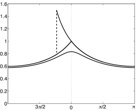
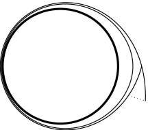
Figure 2: Three steady state solutions of equation (2.2) with $\mu=1$. Left: solutions plotted as $(x,h(x))$. The smooth curve corresponds a steady state with flux $q=0.64$. The discontinuous curve and the curve with a corner in it correspond to the critical flux value $q=2/3$. Right: solutions plotted as a film coating a cylinder of radius $1$. The cylinder is denoted with a heavy line.

Smooth, positive steady states in the presence of surface tension have been studied by a number of authors. One striking computational result [1] is that for certain values of $\chi$ and $\mu$ there can be non-uniqueness. Specifically, one can find flux values $q$ for which there are more than one steady state with that flux (the steady states have different total mass). Similarly, one can find total masses for which there are more than one steady state (the steady states have different flux). These steady states were numerically discovered via an elegant combination of asymptotics and a two-parameter (mass and flux) continuation method [1, Figure 14]. To start the continuation method, earlier work [2] on the regime in which viscous forces dominate gravity was used. There, asymptotics show that for small fluxes the steady state is close to $q+1/3q^{3}\cos(x)+\mathcal{O}(q^{5})$, providing a good first guess for the iteration used to find the steady state. The bifurcation diagram shown in Figure 14 of [1] also suggests that the Moffatt model (1.2) can be considered as the limit of the Pukhnachov model (1.3) as surface tension goes to zero ($\chi\to 0$).

We are not aware of a result that proves that smooth positive steady states exist if and only if $0<q<q^{*}(\mu)$ for some $q^{*}(\mu)$. Pukhnachov proved [29] a nonexistence result: no positive steady states exist if $q>2\sqrt{3/\mu}\simeq 3.464/\sqrt{\mu}$. We improve this, proving that no such solution exists if $q>2/3\,\sqrt{2/\mu}\simeq 0.943/\sqrt{\mu}$.

Proposition 2.1.

There does not exist a strictly positive $2\pi$ periodic solution $h(x)$ of equation (2.1) if $q>2/3\,\sqrt{2/\mu}$.

Proof of Proposition 2.1.

Following Pukhnachov, we start by rescaling the flux to $1$ by introducing $y(x)=h(x)/q$ and introducing the parameters $\gamma=\tfrac{\chi\,q^{3}}{3}$ and $\beta=\tfrac{q^{2}\mu}{3}$. Equation (2.1) transforms to

$$\gamma(y^{\prime\prime\prime}+y^{\prime})=\beta\cos{(x)}-\tfrac{1}{y^{2}}+\tfrac{1}{y^{3}}.$$ (2.3)

The solution $y$ is written as

$$y(x)=a_{0}+a_{1}\cos(x)+a_{2}\sin(x)+v(x)$$ (2.4)

where $v(x)\perp\mbox{span}\{1,\cos(x),\sin(x)\}$ and satisfies

$$\gamma(v^{\prime\prime\prime}+v^{\prime})=\beta\cos{(x)}-\tfrac{1}{y(x)^{2}}+\tfrac{1}{y(x)^{3}}.$$ (2.5)

A solution $v$ exists only if the right-hand side of (2.5) is orthogonal to $\mbox{span}\{1,\cos(x),\sin(x)\}$. As a result,

$$\int\limits_{0}^{2\pi}\left(\tfrac{1}{y(x)^{2}}-\tfrac{1}{y(x)^{3}}\right)\;dx=0$$ (2.6)

$$\int\limits_{0}^{2\pi}\left(\tfrac{1}{y(x)^{2}}-\tfrac{1}{y(x)^{3}}\right)\cos(x)\;dx=\pi\,\beta,$$ (2.7)

Adding equations (2.6) and (2.7) yields

$$\pi\beta =\int\limits_{0}^{2\pi}\left(\tfrac{1}{y(x)^{2}}-\tfrac{1}{y(x)^{3}}\right)\left(1+\cos(x)\right)\;dx$$

$$\hskip 36.135pt\leq\int\limits_{y\geq 1}\left(\tfrac{1}{y(x)^{2}}-\tfrac{1}{y(x)^{3}}\right)\left(1+\cos(x)\right)\;dx.$$

The function $F(y)=1/y^{2}-1/y^{3}$ is bounded above by $4/27$ on $[1,\infty)$ hence

$$\pi\beta\leq\int\limits_{y\geq 1}\tfrac{4}{27}\left(1+\cos(x)\right)\;dx\leq\tfrac{4}{27}\,2\pi.$$

This shows that if there is a steady state then $\beta\leq 8/27$. Recalling the definition of $\beta$, there is no steady state if $q>2/3\,\sqrt{2/\mu}$. ∎

The proof also holds in the case of zero surface tension $\chi=\gamma=0$ and so it is natural that the bound $2/3\,\sqrt{2/\mu}$ is larger than $2/(3\sqrt{\mu})$ (the bound found by Johnson and Moffatt.) Also, we note that numerical simulations that suggest nonexistence of a positive steady state if $q>0.854$ when $\mu=1$ for a large range of surface tension values [20, p. 61]; our bound of $0.943$ is not too far off from this. We close the discussion of steady states by considering their nonlinear stability. This is done via simulations of the initial value problem for different regimes of the PDE. Figure 3 considers the PDE with no advection, $h_{t}+(h^{3}(h_{xxx}+16\,h_{x}))_{x}=0$. The PDE is translation invariant in $x$ and constant steady states are linearly unstable. As a result, any non-constant behaviour observed in a solution starting from constant initial data would be due to growth of round-off error. For this reason, non-constant initial data is chosen: $h_{0}(x)=0.3+0.02\,\cos(x)+0.02\,\cos(2x)$. The $L^{2}$ and $H^{1}$ norms of the resulting solution appear to be converging to limiting values as time passes and long-time limit of the solution appears to be four steady-state droplets of the form $a\cos(4x+\phi)+b$ for appropriate values of $a$, $\phi$, and $b$. Like the PDE, the simulation shown respects the symmetry about $x=\pi$ of the initial data. However, we find that if one computes longer, the symmetry is broken and the solution appears to converge to a profile with three steady droplets. This suggests that the four droplet configuration may be a steady state but it’s an unstable one and accumulated round-off error eventually leads the numerical solution away from it.

Figure 4 shows the evolution from constant initial data for the PDE with nonlinear advection but no linear advection: $h_{t}+(h^{3}(h_{xxx}+16\,h_{x}+8\cos(x)))_{x}=0$. The long-time limit appears to be a steady state which is zero (or nearly zero) on $[0,\pi]$ with the bulk of the fluid contained in a droplet supported within $(\pi,2\pi)$, centred roughly about the bottom of the cylinder ($x=3\pi/2$). Finally, Figure 5 shows the evolution resulting from the same constant initial data for the PDE with both linear and nonlinear advection: $h_{t}+(h^{3}(h_{xxx}+16\,h_{x}+8\cos(x)))_{x}+3h_{x}=0$. The long-time limit appears to be fully wetted cylinder with a steady ‘‘droplet’’ centred slightly past the bottom of the cylinder (here ‘‘past’’ refers to the direction determined by the direction of rotation $\omega$; see Figure 1).

We close by noting that the PDE considered in Figure 5 corresponds to coefficient $a_{3}=3$ in the PDE (1.8). As we increase the value of $a_{3}$ we find there appears to be a critical value past which the solution appears to converge to a time-periodic behaviour rather than a steady state. Specifically, a ‘‘thumping’’ behaviour is observed in which the cylinder is fully wetted but the bulk of the fluid is located in one region. This bulk of fluid moves around the rotating cylinder in a time-periodic manner.

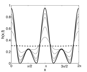
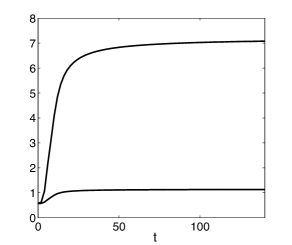
Figure 3: The evolution equation with no linear or nonlinear advection, $h_{t}+(h^{3}(h_{xxx}+16\,h_{x}))_{x}=0$, corresponding to $a_{0}=1$, $a_{1}=16$, and $a_{2}=a_{3}=0$. The initial data is $h_{0}(x)=0.3+0.02\,\cos(x)+0.02\,\cos(2x)$. Left plot: the solution at times $t=0$ (dashed line), $t=12,12.5,13,15$ (solid lines), and $t=140$ (heavy line). Right plot: the $L^{2}$ and $H^{1}$ norms plotted as a function of time.

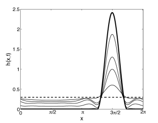
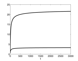
Figure 4: The evolution equation with nonlinear advection but no linear advection, $h_{t}+(h^{3}(h_{xxx}+16\,h_{x}+8\cos(x)))_{x}=0$, corresponding to $a_{0}=1$, $a_{1}=16$, $a_{2}=8$, and $a_{3}=0$. The initial data is $h_{0}(x)=0.3$. Left plot: the solution at times $t=0$ (dashed line), $t=0.5,1,2,10$ (solid lines), and $t=3000$ (heavy line). Right plot: the $L^{2}$ and $H^{1}$ norms plotted as a function of time.

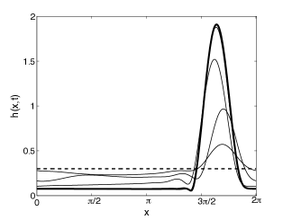
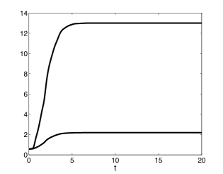
Figure 5: The evolution equation with both linear and nonlinear advection, $h_{t}+(h^{3}(h_{xxx}+16\,h_{x}+8\cos(x)))_{x}+3h_{x}=0$, corresponding to $a_{0}=1$, $a_{1}=16$, $a_{2}=8$, and $a_{3}=3$. The initial data is $h_{0}(x)=0.3$. Left plot: the solution at times $t=0$ (dashed line), $t=0.5,1,2,4$ (solid lines), and $t=20$ (heavy line). Right plot: the $L^{2}$ and $H^{1}$ norms plotted as a function of time.

3 Short–time Existence and Regularity of Solutions

We are interested in the existence of nonnegative generalized weak solutions to the following initial–boundary value problem:

$$(\textup{P}) h_{t}+\left({f(h)(a_{0}h_{xxx}+a_{1}h_{x}+a_{2}w^{\prime}(x))}\right)_{x}+a_{3}h_{x}=0\text{ in }Q_{T},\qquad$$ (3.1)

$$(\textup{P}) \tfrac{\partial^{i}h}{\partial x^{i}}(-a,t)=\tfrac{\partial^{i}h}{\partial x^{i}}(a,t)\text{ for }t>0,\,i=\overline{0,3},$$ (3.2)

$$(\textup{P}) h(x,0)=h_{0}(x)\geqslant 0,$$ (3.3)

where $f(h)=|h|^{3}$, $h=h(x,t)$, $\Omega=(-a,a)$, and $Q_{T}=\Omega\times(0,T)$. Note that rather than considering the interval $(-a,a)$ with boundary conditions (3.2) one can equally well consider the problem on the circle $S^{1}$; our methods and results would apply here too. Recall that $a_{1}$, $a_{2}$, and $a_{3}$ in equation (3.1) are arbitrary constants; $a_{0}$ is required to be positive. The function $w$ in (3.1) is assumed to satisfy:

$$w\in C^{2+\gamma}(\Omega)\;\mbox{for some}\;0<\gamma<1,\tfrac{\partial^{i}w}{\partial x^{i}}(-a)=\tfrac{\partial^{i}w}{\partial x^{i}}(a)\text{ for }i=0,1,2.$$ (3.4)

We consider a generalized weak solution in the following sense [3, 4]:

Definition 3.1.

A generalized weak solution of problem $(\textup{P})$ is a function $h$ satisfying

$$h\in C^{1/2,1/8}_{x,t}(\overline{Q}_{T})\cap L^{\infty}(0,T;H^{1}(\Omega)),$$ (3.5)

$$h_{t}\in L^{2}(0,T;(H^{1}(\Omega))^{\prime}),$$ (3.6)

$$h\in C^{4,1}_{x,t}(\mathcal{P}),\,\,\,\sqrt{f(h)}\,\left(a_{0}h_{xxx}+a_{1}h_{x}+a_{2}w^{\prime}\right)\in L^{2}(\mathcal{P}),\,\,$$ (3.7)

where $\mathcal{P}=\overline{Q}_{T}\setminus({h=0}\cup{t=0})$ and $h$ satisfies (3.1) in the following sense:

$$\int\limits_{0}^{T}\langle h_{t}(\cdot,t),\phi\rangle\;dt-\iint\limits_{\mathcal{P}}{f(h)(a_{0}h_{xxx}+a_{1}h_{x}+a_{2}w^{\prime}(x))\phi_{x}\,dxdt}$$

$$\hskip 180.67499pt-a_{3}\iint\limits_{Q_{T}}{h\phi_{x}\,dxdt}=0$$ (3.8)

for all $\phi\in C^{1}(Q_{T})$ with $\phi(-a,\cdot)=\phi(a,\cdot)$;

$$h(\cdot,t)\to h(\cdot,0)=h_{0}\mbox{ pointwise \& strongly in $L^{2}(\Omega)$ as $t\to 0$},$$ (3.9)

$$h(-a,t)=h(a,t)\;\forall t\in[0,T]\;\mbox{and}\;\tfrac{\partial^{i}h}{\partial x^{i}}(-a,t)=\tfrac{\partial^{i}h}{\partial x^{i}}(a,t)$$ (3.10)

$$\mbox{for}\;i=\overline{1,3}\;\mbox{at all points of the lateral boundary where $\{h\neq 0\}$.}$$

Because the second term of (3.8) has an integral over $\mathcal{P}$ rather than over $Q_{T}$, the generalized weak solution is ‘‘weaker’’ than a standard weak solution. Also note that the first term of (3.8) uses $h_{t}\in L^{2}(0,T;(H^{1}(\Omega))^{\prime})$; this is different from the definition of weak solution first introduced by Bernis and Friedman [5]; there, the first term was the integral of $h\phi_{t}$ integrated over $Q_{T}$.

We first prove the short-time existence of a generalized weak solution and then prove that it can have additional regularity. In Section 4 we prove additional control for the $H^{1}$ norm which then allows us to prove long-time existence.

Theorem 1 (Existence).

Let the nonnegative initial data $h_{0}\in H^{1}(\Omega)$ satisfy

$$\int\limits_{\Omega}{\tfrac{1}{h_{0}(x)}}\;dx<\infty,$$ (3.11)

and either 1) $h_{0}(-a)=h_{0}(a)=0$ or 2) $h_{0}(-a)=h_{0}(a)\neq 0$ and $\tfrac{\partial^{i}h_{0}}{\partial x^{i}}(-a)=\tfrac{\partial^{i}h_{0}}{\partial x^{i}}(a)\text{ holds for }i=1,2,3$. Then for some time $T_{loc}>0$ there exists a nonnegative generalized weak solution, $h$, on $Q_{T_{loc}}$ in the sense of the definition 3.1. Furthermore,

$$h\in L^{2}(0,T_{loc};H^{2}(\Omega)).$$ (3.12)

Let

$$\mathcal{E}_{0}(T):=\tfrac{1}{2}\int\limits_{\Omega}({a_{0}h_{x}^{2}(x,T)-a_{1}h^{2}(x,T)-2a_{2}w(x)h(x,T))\,dx},$$ (3.13)

and

$$B_{0}(T):=2\left(\tfrac{a_{1}^{2}}{a_{0}}+\tfrac{a_{2}^{2}}{a_{0}}\mathop{\|}w^{\prime}\|_{\infty}^{2}\right)\int\limits_{0}^{T}{\|h(\cdot,t)\|^{3}_{L^{\infty}(\Omega)}\,dt}.$$

then the weak solution satisfies

$$\mathcal{E}_{0}(T_{loc})+\iint\limits_{\{h>0\}}{h^{3}(a_{0}h_{xxx}+a_{1}h_{x}+a_{2}w^{\prime})^{2}\,dx\,dt}\leqslant\mathcal{E}_{0}(0)+K\,T_{loc},$$ (3.14)

and

$$\int\limits_{\Omega}{h_{x}^{2}(x,T_{loc})\,dx}\leqslant e^{B_{0}(T_{loc})}\int\limits_{\Omega}{h_{0x}^{2}(x)\,dx}$$ (3.15)

where $K=|a_{2}a_{3}|\,\|w^{\prime}\|_{\infty}C<\infty$. The time of existence, $T_{loc}$, is determined by $a_{0}$, $a_{1}$, $a_{2}$, $\|w^{\prime}\|_{2}$, $\|w^{\prime}\|_{\infty}$, $|\Omega|$, $\int h_{0}$, $\|h_{0x}\|_{2}$, and $\int 1/h_{0}$.

There is nothing special about the time $T_{loc}$ in the bounds (3.14) and (3.15); given a countable collection of times in $[0,T_{loc}]$, one can construct a weak solution for which these bounds will hold at those times. Also, we note that the analogue of Theorem 4.2 in [5] also holds: there exists a nonnegative weak solution with the integral formulation

$$\int\limits_{0}^{T}\langle h_{t}(\cdot,t),\phi\rangle\;dt+a_{0}\iint\limits_{Q_{T}}(3h^{2}h_{x}h_{xx}\phi_{x}+h^{3}h_{xx}\phi_{xx})\;dxdt$$ (3.16)

$$\hskip 108.405pt-\iint\limits_{Q_{T}}\left(a_{1}h_{x}+a_{2}w^{\prime}+a_{3}h\right)\phi_{x}\;dxdt=0.$$

Theorem 2 (Regularity).

If the initial data from Theorem 1 also satisfies

$$\int\limits_{\Omega}{h_{0}^{\alpha-1}(x)\,dx}<\infty$$

for some $-1/2<\alpha<1,\quad\alpha\neq 0$ then there exists $0<T_{loc}^{(\alpha)}\leq T_{loc}$ such that the nonnegative generalized weak solution from Theorem 1 has the extra regularity $h^{\tfrac{\alpha+2}{2}}\in L^{2}(0,T_{loc}^{(\alpha)};H^{2}(\Omega))$ and $h^{\tfrac{\alpha+2}{4}}\in L^{2}(0,T_{loc}^{(\alpha)};W^{1}_{4}(\Omega))$.

The solutions from Theorem 2 are often called ‘‘strong’’ solutions in the thin film literature. If the initial data satisfies $\int h_{0}^{\alpha-1}\;dx<\infty$ then the added regularity from Theorem 2 allows one to prove the existence of nonnegative solutions with an integral formulation [7] that is similar to that of (3.16) except that the second integral is replaced by the results of one more integration by parts (there are no $h_{xx}$ terms). We also note that if one considered problem (P) with nonlinearity $f(h)=|h|^{n}$ with $0<n<3$, then Theorems 1 and 2 would hold for general nonnegative initial data $h_{0}\in H^{1}(\Omega)$; no ‘‘finite entropy’’ assumption would be needed [7, 3]. Finite entropy conditions ($\int h_{0}^{2-n}\;dx<\infty$ and $\int h_{0}^{\alpha+2-n}\;dx<\infty$) would be needed to obtain the results for $n\geq 3$.

3.1 Regularized Problem

Given $\delta,\varepsilon>0$, a regularized parabolic problem, similar to that of Bernis and Friedman [5], is considered:

$$(\textup{P}_{\delta,\epsilon}) h_{t}+\left({f_{\delta\varepsilon}(h)\bigl{(}a_{0}h_{xxx}+a_{1}h_{x}+a_{2}w^{\prime}(x)\bigr{)}}\right)_{x}+a_{3}h_{x}=0,\qquad\hfill$$ (3.17)

$$(\textup{P}_{\delta,\epsilon}) \tfrac{\partial^{i}h}{\partial x^{i}}(-a,t)=\tfrac{\partial^{i}h}{\partial x^{i}}(a,t)\text{ for }t>0,\,i=0,1,2,3,\hfill$$ (3.18)

$$(\textup{P}_{\delta,\epsilon}) \qquad\qquad h(x,0)=h_{0,\delta\varepsilon}(x)\hfill$$ (3.19)

where

$$f_{\delta\varepsilon}(z):=f_{\varepsilon}(z)+\delta=\tfrac{|z|^{4}}{|z|+\varepsilon}+\delta\quad\ \forall\,z\in\mathbb{R}^{1},\ \delta>0,\varepsilon>0.$$ (3.20)

The $\delta>0$ in (3.20) makes the problem (3.17) regular (i.e. uniformly parabolic). The parameter $\varepsilon$ is an approximating parameter which has the effect of increasing the degeneracy from $f(h)\sim|h|^{3}$ to $f_{\varepsilon}(h)\sim h^{4}$. The nonnegative initial data, $h_{0}$, is approximated via

$$\begin{gathered}h_{0,\delta\varepsilon}=h_{0,\delta}+\varepsilon^{\theta}\in C^{4+\gamma}(\Omega)\text{ for some }0<\theta<2/5\text{ and }\gamma\text{ from }(\ref{B:w})\\ \tfrac{\partial^{i}h_{0,\delta\varepsilon}}{\partial x^{i}}(-a)=\tfrac{\partial^{i}h_{0,\delta\varepsilon}}{\partial x^{i}}(a)\text{ for }i=\overline{0,3},\\ h_{0,\delta\varepsilon}\to h_{0}\text{ strongly in }H^{1}(\Omega)\text{ as }\delta,\varepsilon\to 0.\end{gathered}$$ (3.21)

The $\varepsilon$ term in (3.21) ‘‘lifts’’ the initial data so that it will be positive even if $\delta=0$ and the $\delta$ is involved in smoothing the initial data from $H^{1}(\Omega)$ to $C^{4+\gamma}(\Omega)$.

By Eĭdelman [16, Theorem 6.3, p.302], the regularized problem has a unique classical solution $h_{\delta\varepsilon}\in C_{x,t}^{4+\gamma,1+\gamma/4}(\Omega\times[0,\tau_{\delta\varepsilon}])$ for some time $\tau_{\delta\varepsilon}>0$. For any fixed value of $\delta$ and $\varepsilon$, by Eĭdelman [16, Theorem 9.3, p.316] if one can prove a uniform in time an a priori bound $|h_{\delta\varepsilon}(x,t)|\leq A_{\delta\varepsilon}<\infty$ for some longer time interval $[0,T_{loc,\delta\varepsilon}]\quad(T_{loc,\delta\varepsilon}>\tau_{\delta\varepsilon}$) and for all $x\in\Omega$ then Schauder-type interior estimates [16, Corollary 2, p.213] imply that the solution $h_{\delta\varepsilon}$ can be continued in time to be in $C_{x,t}^{4+\gamma,1+\gamma/4}(\Omega\times[0,T_{loc,\delta\varepsilon}])$.

Although the solution $h_{\delta\varepsilon}$ is initially positive, there is no guarantee that it will remain nonnegative. The goal is to take $\delta\to 0$, $\epsilon\to 0$ in such a way that 1) $T_{loc,\delta\varepsilon}\to T_{loc}>0$, 2) the solutions $h_{\delta\varepsilon}$ converge to a (nonnegative) limit, $h$, which is a generalized weak solution, and 3) $h$ inherits certain a priori bounds. This is done by proving various a priori estimates for $h_{\delta\varepsilon}$ that are uniform in $\delta$ and $\varepsilon$ and hold on a time interval $[0,T_{loc}]$ that is independent of $\delta$ and $\varepsilon$. As a result, $\{h_{\delta\varepsilon}\}$ will be a uniformly bounded and equicontinuous (in the $C_{x,t}^{1/2,1/8}$ norm) family of functions in $\bar{\Omega}\times[0,T_{loc}]$. Taking $\delta\to 0$ will result in a family of functions $\{h_{\varepsilon}\}$ that are classical, positive, unique solutions to the regularized problem with $\delta=0$. Taking $\varepsilon\to 0$ will then result in the desired generalized weak solution $h$. This last step is where the possibility of nonunique weak solutions arise; see [3] for simple examples of how such constructions applied to $h_{t}=-(|h|^{n}h_{xxx})_{x}$ can result in two different solutions arising from the same initial data.

3.2 A priori estimates

Our first task is to derive a priori estimates for classical solutions of (3.17)–(3.21). The lemmas in this section are proved in Section A.

We use an integral quantity based on a function $G_{\delta\varepsilon}$ chosen so that

$$G^{\prime\prime}_{\delta\varepsilon}(z)=\tfrac{1}{f_{\delta\varepsilon}(z)}\quad\mbox{and}\quad G_{\delta\varepsilon}(z)\geq 0.$$ (3.22)

This is analogous to the ‘‘entropy’’ function first introduced by Bernis and Friedman [5].

Lemma 3.1.

There exists $\delta_{0}>0$, $\varepsilon_{0}>0$, and time $T_{loc}>0$ such that if $\delta\in[0,\delta_{0})$, $\varepsilon\in(0,\varepsilon_{0})$, if $h_{\delta\varepsilon}$ is a classical solution of the problem (3.17)–(3.21) with initial data $h_{0,\delta\varepsilon}$, and if $h_{0,\delta\varepsilon}$ satisfies (3.21) and is built from a nonnegative function $h_{0}$ that satisfies the hypotheses of Theorem 1 then for any $T\in[0,T_{loc}]$ the solution $h_{\delta\varepsilon}$ satisfies

$$\int\limits_{\Omega}{\{h_{\delta\varepsilon,x}^{2}(x,T)+\tfrac{|a_{1}|}{a_{0}}\left(\tfrac{|a_{1}|}{a_{0}}+2\delta\right)G_{\delta\varepsilon}(h_{\delta\varepsilon}(x,T))\}\,dx}$$ (3.23)

$$\hskip 72.26999pt+a_{0}\iint\limits_{Q_{T}}{f_{\delta\varepsilon}(h_{\delta\varepsilon})h^{2}_{\delta\varepsilon,xxx}\,dxdt}\leqslant K_{1}<\infty,$$

$$\int\limits_{\Omega}G_{\delta\varepsilon}(h_{\delta\varepsilon}(x,T))\;dx+a_{0}\iint\limits_{Q_{T}}h_{\delta\varepsilon,xx}^{2}\;dxdt\leq K_{2}<\infty,$$ (3.24)

and the energy $\mathcal{E}_{\delta\varepsilon}(t)$ (see (3.13)) satisfies:

$$\mathcal{E}_{\delta\varepsilon}(T)+\iint\limits_{Q_{T}}{f_{\delta\varepsilon}(h_{\delta\varepsilon})(a_{0}h_{\delta\varepsilon,xxx}+a_{1}h_{\delta\varepsilon,x}+a_{2}w^{\prime})^{2}}\;dxdt$$ (3.25)

$$\hskip 216.81pt\leqslant C_{0}+K_{3}T$$

where $K_{3}=|a_{2}a_{3}|\mathop{\|}w^{\prime}\|_{\infty}C<\infty$. The time $T_{loc}$ and the constants $K_{1}$, $K_{2}$, $C_{0}$, and $K_{3}$ are independent of $\delta$ and $\varepsilon$.

The existence of $\delta_{0}$, $\varepsilon_{0}$, $T_{loc}$, $K_{1}$, $K_{2}$, and $K_{3}$ is constructive; how to find them and what quantities determine them is shown in Section A.

Lemma 3.1 yields uniform-in-$\delta$-and-$\varepsilon$ bounds for $\int h_{\delta\varepsilon,x}^{2}$, $\int G_{\delta\varepsilon}(h_{\delta\varepsilon})$, $\iint h_{\delta\varepsilon,xx}^{2}$, and
$\iint f_{\delta\varepsilon}(h_{\delta\varepsilon})h_{\delta\varepsilon,xxx}^{2}$. However, these bounds are found in a different manner than in earlier work for the equation $h_{t}=-(|h|^{n}h_{xxx})_{x}$, for example. Although the inequality (3.24) is unchanged, the inequality (3.23) has an extra term involving $G_{\delta\varepsilon}$. In the proof, this term was introduced to control additional, lower–order terms. This idea of a ‘‘blended’’ $\|h_{x}\|_{2}$–entropy bound was first introduced by Shishkov and Taranets especially for long-wave stable thin film equations with convection [30].

Lemma 3.2.

Assume $\varepsilon_{0}$ and $T_{loc}$ are from Lemma 3.1, $\delta=0$, and $\varepsilon\in(0,\varepsilon_{0})$. If $h_{\varepsilon}$ is a positive, classical solution of the problem (3.17)–(3.21) with initial data $h_{0,\varepsilon}$ satisfying Lemma 3.1.

$$\int\limits_{\Omega}{h_{\varepsilon,x}^{2}(x,T)\,dx}\leq\max\left\{\|w^{\prime}\|_{2}^{2},\int\limits_{\Omega}h_{0\varepsilon,x}^{2}\,dx\right\}e^{B_{\varepsilon}(T)}$$ (3.26)

holds true for all $T\in[0,T_{loc}]$. Here

$$B_{\varepsilon}(T):=2\tfrac{a_{1}^{2}+a_{2}^{2}}{a_{0}}\int\limits_{0}^{T}\|h_{\varepsilon}(\cdot,t)\|_{\infty}^{3}\;dt$$

The final a priori bound uses the following functions, parametrized by $\alpha$,

$$G_{\varepsilon}^{(\alpha)}(z):=\tfrac{z^{\alpha-1}}{(\alpha-1)(\alpha-2)}+\tfrac{\varepsilon z^{\alpha-2}}{(\alpha-3)(\alpha-2)};\ (G^{(\alpha)}_{\varepsilon}(z))^{\prime\prime}=\tfrac{z^{\alpha}}{f_{\varepsilon}(z)}.$$ (3.27)

Lemma 3.3.

Assume $\varepsilon_{0}$ and $T_{loc}$ are from Lemma 3.1, $\delta=0$, and $\varepsilon\in(0,\varepsilon_{0})$. Assume $h_{\varepsilon}$ is a positive, classical solution of the problem (3.17)–(3.21) with initial data $h_{0,\varepsilon}$ satisfying Lemma 3.1. Fix $\alpha\in(-1/2,1)$ with $\alpha\neq 0$. If the initial data $h_{0,\varepsilon}$ is built from $h_{0}$ which also satisfies

$$\int\limits_{\Omega}h_{0}^{\alpha-1}(x)\;dx<\infty$$ (3.28)

then there exists $\varepsilon_{0}^{(\alpha)}$ and $T_{loc}^{(\alpha)}$ with $0<\varepsilon_{0}^{(\alpha)}\leq\varepsilon_{0}$ and $0<T_{loc}^{(\alpha)}\leq T_{loc}$ such that

$$\int\limits_{\Omega}{\{h_{\varepsilon,x}^{2}(x,T)+G_{\varepsilon}^{(\alpha)}(h_{\varepsilon}(x,T))\}\,dx}$$ (3.29)

$$\hskip 72.26999pt+\iint\limits_{Q_{T}}\left[\beta h_{\varepsilon}^{\alpha}h_{\varepsilon,xx}^{2}+\gamma h_{\varepsilon}^{\alpha-2}h_{\varepsilon,x}^{4}\right]\;dx\,dt\leqslant K_{4}<\infty$$

holds for all $T\in[0,T_{loc}^{(\alpha)}]$ and some constant $K_{4}$ that is determined by $\alpha$, $\varepsilon_{0}$, $a_{0}$, $a_{1}$, $a_{2}$, $w^{\prime}$, $\Omega$ and $h_{0}$. Here,

$$\beta=\begin{cases}a_{0}&\mbox{if }0<\alpha<1,\\ a_{0}\tfrac{1+2\alpha}{4(1-\alpha)}&\mbox{if }-1/2<\alpha<0\end{cases}$$

and

$$\gamma=\begin{cases}a_{0}\tfrac{\alpha(1-\alpha)}{6}&\mbox{if }0<\alpha<1,\\ a_{0}\tfrac{(1+2\alpha)(1-\alpha)}{36}&\mbox{if }-1/2<\alpha<0.\end{cases}$$

Furthermore,

$$h_{\varepsilon}^{\tfrac{\alpha+2}{2}}\in L^{2}(0,T_{loc};H^{2}(\Omega))\quad\mbox{and}\quad h_{\varepsilon}^{\tfrac{\alpha+2}{4}}\in L^{2}(0,T_{loc};W^{1}_{4}(\Omega))$$ (3.30)

with a uniform-in-$\varepsilon$ bound.

The $\alpha$–entropy, $\int G_{0}^{(\alpha)}(h)\;dx$, was first introduced for $\alpha=-1/2$ in [10] and an a priori bound like that of Lemma 3.3 and regularity results like those of Theorem 2 were found simultaneously and independently in [3] and [7].

3.3 Proof of existence and regularity of solutions

Bound (3.23) yields uniform $L^{\infty}$ control for classical solutions $h_{\delta\varepsilon}$, allowing the time of existence $T_{loc,\delta\varepsilon}$ to be taken as $T_{loc}$ for all $\delta\in(0,\delta_{0})$ and $\varepsilon\in(0,\varepsilon_{0})$. The existence theory starts by constructing a classical solution $h_{\delta\varepsilon}$ on $[0,T_{loc}]$ that satisfy the hypotheses of Lemma 3.1 if $\delta\in(0,\delta_{0})$ and $\varepsilon\in(0,\varepsilon_{0})$. The regularizing parameter, $\delta$, is taken to zero and one proves that there is a limit $h_{\varepsilon}$ and that $h_{\varepsilon}$ is a generalized weak solution. One then proves additional regularity for $h_{\varepsilon}$; specifically that it is strictly positive, classical, and unique. It then follows that the a priori bounds given by Lemmas 3.1, and 3.3 apply to $h_{\varepsilon}$. This allows us to take the approximating parameter, $\varepsilon$, to zero and construct the desired generalized weak solution of Theorems 1 and 2.

Lemma 3.4.

Assume that the initial data $h_{0,\varepsilon}$ satisfies (3.21) and is built from a nonnegative function $h_{0}$ that satisfies the hypotheses of Theorem 1. Fix $\delta=0$ and $\varepsilon\in(0,\varepsilon_{0})$ where $\varepsilon_{0}$ is from Lemma 3.1. Then there exists a unique, positive, classical solution $h_{\varepsilon}$ on $[0,T_{loc}]$ of problem ($\mbox{P}_{0,\varepsilon}$), see (3.17)–(3.21), with initial data $h_{0,\varepsilon}$ where $T_{loc}$ is the time from Lemma 3.1.

The proof uses a number of arguments like those presented by Bernis & Friedman [5] and we refer to that article as much as possible.

Proof.

Fix $\varepsilon\in(0,\varepsilon_{0})$ and assume $\delta\in(0,\delta_{0})$. Because $G_{\delta\varepsilon}(z)\geq 0$, the bound (3.23) yields a uniform-in-$\delta$-and-$\varepsilon$ upper bound on $|h_{\delta\varepsilon}(x,T)|$ for $(x,T)\in\overline{\Omega}\times[0,T_{loc}]$. As discussed in Subsection 3.1, this allows the classical solution $h_{\delta\varepsilon}$ to be extended from $[0,\tau_{\delta\varepsilon}]$ to $[0,T_{loc}]$.

By Section 2 of [5], the a priori bound (3.23) on $\|h_{x}(\cdot,T)\|_{2}$ implies that $h_{\delta\varepsilon}\in C^{1/2,1/8}_{x,t}(\overline{Q_{T_{loc}}})$ and that $\{h_{\delta\varepsilon}\}$ is a uniformly bounded, equicontinuous family in $\overline{Q_{T_{loc}}}$. By the Arzela-Ascoli theorem, there is a subsequence $\{\delta_{k}\}$, so that $h_{\delta_{k}\varepsilon}$ converges uniformly to a limit $h_{\varepsilon}\in C^{1/2,1/8}_{x,t}(\overline{Q_{T_{loc}}})$.

We now argue that $h_{\varepsilon}$ is a generalized weak solution, using methods similar to those of [5, Theorem 3.1].

By construction, $h_{\varepsilon}$ is in $C^{1/2,1/8}_{x,t}(\overline{Q_{T_{loc}}})$, satisfying the first part of (3.5). The strong convergence $h_{\varepsilon}(\cdot,t)\to h_{\varepsilon}(\cdot,0)$ in $L^{2}(\Omega)$ follows immediately. The uniform convergence of $h_{\delta_{k}\varepsilon}$ to $h_{\varepsilon}$ implies the pointwise convergence $h(\cdot,t)\to h(\cdot,0)=h_{0}$, and so $h_{\varepsilon}$ satisfies (3.9).

Because $h_{\delta\varepsilon}$ is a classical solution,

$$\iint\limits_{Q_{T}}{h_{\delta\varepsilon}\phi\;dxdt}-\iint\limits_{Q_{T_{loc}}}{f_{\delta\varepsilon}(h_{\delta\varepsilon})(a_{0}h_{\delta\varepsilon,xxx}+a_{1}h_{\delta\varepsilon,x}+a_{2}w^{\prime}(x))\phi_{x}\;dxdt}$$

$$\hskip 180.67499pt-a_{3}\iint\limits_{Q_{T_{loc}}}{h_{\delta\varepsilon}\phi_{x}\;dxdt}=0.$$ (3.31)

The bound (3.23) yields a uniform bound on

$$\delta\iint\limits_{Q_{T_{loc}}}h_{\delta\varepsilon,xxx}^{2}\;dxdt$$

for $\delta\in(0,\delta_{0})$. It follows that

$$\delta_{k}\iint\limits_{Q_{T_{loc}}}(a_{0}h_{\delta\varepsilon,xxx}+a_{1}h_{\delta\varepsilon,x}+a_{2}w^{\prime}(x))\phi_{x}\,dxdt\to 0\qquad\mbox{as $\delta_{k}\to 0$.}$$

Introducing the notation

$$H_{\delta\varepsilon}:=f_{\delta\varepsilon}(h_{\delta\varepsilon})(a_{0}h_{\delta\varepsilon,xxx}+a_{1}h_{\delta\varepsilon,x}+a_{2}w^{\prime}(x))+a_{3}h_{\delta\varepsilon}$$ (3.32)

the integral formulation (3.31) can be written as

$$\iint\limits_{Q_{T}}{h_{\delta\varepsilon}\phi dxdt}=\iint\limits_{Q_{T_{loc}}}H_{\delta\varepsilon}(x,t)\phi_{x}(x,t)\;dxdt.$$ (3.33)

By the $L^{\infty}$ control of $h_{\delta\varepsilon}$ and the energy bound (3.25), $H_{\delta\varepsilon}$ is uniformly bounded in $L^{2}(Q_{T_{loc}})$. Taking a further subsequence of $\{\delta_{k}\}$ yields $H_{\delta_{k}\varepsilon}$ converging weakly to a function $H_{\varepsilon}$ in $L^{2}(Q_{T_{loc}})$. The regularity theory for uniformly parabolic equations implies that $h_{\delta\varepsilon,t}$, $h_{\delta\varepsilon,x}$, $h_{\delta\varepsilon,xx}$, $h_{\delta\varepsilon,xxx}$, and $h_{\delta\varepsilon,xxxx}$ converge uniformly to $h_{\varepsilon,t}$, …, $h_{\varepsilon,xxxx}$ on any compact subset of $\{h_{\varepsilon}>0\}$, implying (3.10) and the first part of (3.7). Note that because the initial data $h_{0,\varepsilon}$ is in $C^{4}$ the regularity extends all the way to $t=0$ which is excluded in the definition of $\mathcal{P}$ in (3.7).

The energy $\mathcal{E}_{\delta\varepsilon}(T_{loc})$ is not necessarily positive. However, the a priori bound (3.23), combined with the $L^{\infty}$ control on $h_{\delta\varepsilon}$, ensures that $\mathcal{E}_{\delta\varepsilon}(T_{loc})$ has a uniform lower bound. As a result, the bound (3.25) yields a uniform bound on

$$\iint\limits_{Q_{T_{loc}}}f_{\delta\varepsilon}\left(h_{\delta\varepsilon})(a_{0}h_{\delta\varepsilon,xxx}+a_{1}h_{\delta\varepsilon,x}+a_{2}w^{\prime}(x)\right)^{2}\;dxdt.$$

Using this, one can argue that for any $0<\sigma$

$$\iint\limits_{\{h_{\varepsilon}<\sigma\}}\left|H_{\delta_{k}\varepsilon}\phi_{x}\right|\;dxdt\leq C\sigma^{3/2}$$

for some $C$ independent of $\delta$, $\varepsilon$, and $\sigma$. Taking $\delta_{k}\to 0$ and using that $\sigma$ is arbitrary, we conclude

$$H_{\delta_{k}\varepsilon}\to H_{\varepsilon}=f_{\varepsilon}\left(h_{\varepsilon})(a_{0}h_{\varepsilon,xxx}+a_{1}h_{\varepsilon,x}+a_{2}w^{\prime}(x)\right)\,\chi\raisebox{-6.45831pt}{\scriptsize$\{h_{\varepsilon}>0\}$}+a_{3}h_{\varepsilon}.$$

As a result, taking $\delta_{k}\to 0$ in (3.33) implies $h_{\varepsilon}$ satisfies (3.8).

The bound (3.23) yields a uniform bound on $\iint f_{\delta\varepsilon}(h_{\delta\varepsilon})h_{\delta\varepsilon,xxx}^{2}$ which can be used in a similar manner as above to argue that the second part of (3.7) holds. The bound (3.23) also yields a uniform bound on $\int h_{\delta\varepsilon.x}^{2}(x,T)\;dx$ for every $T\in[0,T_{loc}]$. As a result, $\{h_{\delta_{k}\varepsilon}\}$ is uniformly bounded in

$$L^{\infty}(0,T_{loc};H^{1}(\Omega)).$$

Therefore, another refinement of the sequence $\{\delta_{k}\}$ yields $\{h_{\delta_{k}\varepsilon}\}$ weakly convergent in this space. As a result, $h_{\varepsilon}\in L^{\infty}(0,T_{loc};H^{1}(\Omega))$ and the second part of (3.5) holds.

Having proven then $h_{\varepsilon}$ is a generalized weak solution, we now prove that $h_{\varepsilon}$ is a strictly positive, classical, unique solution. This uses the entropy $\int G_{\delta\varepsilon}(h_{\delta\varepsilon})$ and the a priori bound (3.24). This bound is, up to the coefficient $a_{0}$, identical to the a priori bound (4.17) in [5]. By construction, the initial data $h_{0,\varepsilon}$ is positive (see (3.21)), hence $\int G_{\varepsilon}(h_{0,\varepsilon})\;dx<\infty$. Also, by construction $f_{\varepsilon}(z)\sim z^{4}$. for $z\ll 1$ This implies that the generalized weak solution $h_{\varepsilon}$ is strictly positive [5, Theorem 4.1]. Because the initial data $h_{0,\varepsilon}$ is in $C^{4}(\Omega)$, it follows that $h_{\varepsilon}$ is a classical solution in $C^{4,1}_{x,t}(\overline{Q_{T_{loc}}})$. This implies that $h_{\varepsilon}(\cdot,t)\to h_{\varepsilon}(\cdot,0)$ strongly in $C^{1}(\bar{\Omega})$. The proof of Theorem 4.1 in [5] then implies that $h_{\varepsilon}$ is unique. ∎

Proof of Theorem 1.

As in the proof of Lemma 3.4, following [5], there is a subsequence $\{\varepsilon_{k}\}$ such that $h_{\varepsilon_{k}}$ converges uniformly to a function $h\in C^{1/2,1/8}_{x,t}$ which is a generalized weak solution in the sense of Definition 3.1 with $f(h)=|h|^{3}$.

The initial data is assumed to have finite entropy: $\int 1/h_{0}<\infty$. This, combined with $f(h)=|h|^{3}$, implies that the generalized weak solution $h$ is nonnegative and the set of points $\{h=0\}$ in $Q_{T_{loc}}$ has zero measure [5, Theorem 4.1].

To prove (3.14), start by taking $T=T_{loc}$ in the a priori bound (3.25). As $\varepsilon_{k}\to 0$, the right-hand side of (3.25) is unchanged. First, consider the $\varepsilon_{k}\to 0$ limit of

$$\mathcal{E}_{\varepsilon_{k}}(T_{loc})=\tfrac{1}{2}\int\limits_{\Omega}{(a_{0}h_{\varepsilon_{k},x}^{2}(x,T_{loc})-a_{1}h_{\varepsilon_{k}}^{2}(x,T_{loc})-2a_{2}w(x)h_{\varepsilon_{k}}(x,T_{loc}))\,dx}.$$

By the uniform convergence of $h_{\varepsilon_{k}}$ to $h$, the second and third terms in the energy converge strongly as $\varepsilon_{k}\to 0$. The bound (3.25) yields a uniform bound on $\{\int_{\Omega}h_{\varepsilon_{k},x}^{2}(x,T_{loc})\;dx\}$. Taking a further refinement of $\{\varepsilon_{k}\}$, yields $h_{\varepsilon_{k},x}(\cdot,T_{loc})$ converging weakly in $L^{2}(\Omega)$. In a Hilbert space, the norm of the weak limit is less than or equal to the $\liminf$ of the norms of the functions in the sequence, hence $\mathcal{E}_{0}(T_{loc})\leq\liminf_{\varepsilon_{k}\to 0}\mathcal{E}_{\varepsilon_{k}}(T_{loc}).$ A uniform bound on $\iint f_{\varepsilon}(h_{\varepsilon})\left(a_{0}h_{\varepsilon,xxx}+\dots\right)^{2}\;dx$ also follows from (3.25). Hence $\sqrt{f_{\varepsilon_{k}}(h_{\varepsilon_{k}})}\left(a_{0}h_{\varepsilon_{k},xxx}+\dots\right)$ converges weakly in $L^{2}(Q_{T_{loc}})$, after taking a further subsequence. It suffices to determine the weak limit up to a set of measure zero. Because $h\geq 0$ and $\{h=0\}$ has measure zero, it suffices to determine the weak limit on $\{h>0\}$. As in the proof of Lemma 3.4, the regularity theory for uniformly parabolic equations allows one to argue that the weak limit is $h^{3/2}\left(a_{0}h_{xxx}+\dots\right)$ on $\{h>0\}$. Using that 1) the norm of the weak limit is less than or equal to the $\liminf$ of the norms of the functions in the sequence and that 2) the $\liminf$ of a sum is greater than or equal to the sum of the $\liminf$s, results in the desired bound (3.14).

It follows from (3.24) that $h_{\varepsilon_{k},xx}$ converges weakly to some $v$ in $L^{2}(Q_{T_{loc}})$, combining with strong convergence in $L^{2}(0,T;H^{1}(\Omega))$ of $h_{\varepsilon_{k}}$ to $h$ by Lemma B.1 and with the definition of weak derivative, we obtain that $v=h_{xx}$ and $h\in L^{2}(0,T_{loc};$ $H^{2}(\Omega))$ that implies (3.12). Hence $h_{\varepsilon,t}\to h_{t}\text{ weakly in }L^{2}(0,T;(H^{1}(\Omega))^{\prime})$ that implies (3.6). By Lemma B.2 we also have $h\in C([0,T_{loc}],L^{2}(\Omega))$. ∎

Proof of Theorem 2.

Fix $\alpha\in(-1/2,1)$. The initial data $h_{0}$ is assumed to have finite entropy $\int G_{0}^{(\alpha)}(h_{0}(x))\;dx<\infty$, hence Lemma 3.3 holds for the approximate solutions $\{h_{\varepsilon_{k}}\}$ where this sequence of approximate solutions is assumed to be the one at the end of the proof of Theorem 1. By (3.30),

$$\left\{h_{\varepsilon_{k}}^{\tfrac{\alpha+2}{2}}\right\}\quad\mbox{is uniformly bounded in $\varepsilon_{k}$ in $L^{2}(0,T_{loc};H^{2}(\Omega))$}$$

and

$$\left\{h_{\varepsilon_{k}}^{\tfrac{\alpha+2}{4}}\right\}\quad\mbox{is uniformly bounded in $\varepsilon_{k}$ in $L^{2}(0,T_{loc};W^{1}_{4}(\Omega))$}.$$

Taking a further subsequence in $\{\varepsilon_{k}\}$, it follows from the proof of [14, Lemma 2.5, p.330], these sequences converge weakly in $L^{2}(0,T_{loc};H^{2}(\Omega))$ and $L^{2}(0,T_{loc};W^{1}_{4}(\Omega))$, to $h^{\tfrac{\alpha+2}{2}}$ and $h^{\tfrac{\alpha+2}{4}}$ respectively. ∎

4 Long–time existence of solutions

Lemma 4.1.

Let $h\in H^{1}(\Omega)$ be a nonnegative function such that $\int\limits_{\Omega}{h(x)\,dx}=M>0$. Then

$$\|h\|_{L^{2}(\Omega)}^{2}\leqslant 6^{\tfrac{2}{3}}M^{\tfrac{4}{3}}\biggl{(}\int\limits_{\Omega}{h^{2}_{x}\,dx}\biggr{)}^{\tfrac{1}{3}}+\tfrac{M^{2}}{|\Omega|}.$$ (4.1)

Note that by taking $h$ to be a constant function, one finds that the constant $M^{2}/|\Omega|$ in (4.1) is sharp.

Proof.

Let $v=h-M/|\Omega|$. By (A.3),

$$\|v\|_{L^{2}(\Omega)}^{2}\leqslant(\tfrac{3}{2})^{\tfrac{2}{3}}\biggl{(}\int\limits_{\Omega}{v^{2}_{x}\,dx}\biggr{)}^{\tfrac{1}{3}}\biggl{(}\int\limits_{\Omega}{|v|\,dx}\biggr{)}^{\tfrac{4}{3}}\$$

Hence

$$\|h\|_{L^{2}(\Omega)}^{2}\leqslant(\tfrac{3}{2})^{\tfrac{2}{3}}\biggl{(}\int\limits_{\Omega}{h^{2}_{x}\,dx}\biggr{)}^{\tfrac{1}{3}}\biggl{(}\int\limits_{\Omega}{\left|h-\tfrac{M}{|\Omega|}\right|\,dx}\biggr{)}^{\tfrac{4}{3}}+\tfrac{M^{2}}{|\Omega|}\leqslant\\ (\tfrac{3}{2})^{\tfrac{2}{3}}\biggl{(}\int\limits_{\Omega}{h^{2}_{x}\,dx}\biggr{)}^{\tfrac{1}{3}}(2M)^{\tfrac{4}{3}}+\tfrac{M^{2}}{|\Omega|}.$$

∎

Lemma 4.1 and the bound (3.14) are used to prove $H^{1}$ control of the generalized weak solution constructed in Theorem 1.

Lemma 4.2.

Let $h$ be the generalized solution of Theorem 1. Then

$$\tfrac{a_{0}}{4}\;\|h(\cdot,T_{loc})\|_{H^{1}(\Omega)}^{2}\leq\mathcal{E}_{0}(0)+KT_{loc}+K_{3}$$ (4.2)

where $\mathcal{E}_{0}(0)$ is defined in (3.13), $M=\int h_{0}$, $K=|a_{2}a_{3}|\|w^{\prime}\|_{\infty}C$ and

$$K_{3}=\begin{cases}|a_{2}|\|w\|_{\infty}M&\mbox{ if }a_{0}+a_{1}\leq 0,\\ |a_{2}|\|w\|_{\infty}M+M^{2}\,\left(\frac{2\sqrt{6}\,(a_{0}+a_{1})^{3/2}}{3\sqrt{a_{0}}}+\tfrac{a_{0}+a_{1}}{2|\Omega|}\right)&\mbox{ otherwise}.\end{cases}$$

Note that if the evolution is missing either linear or nonlinear advection ($a_{2}=0$ or $w^{\prime}=0$ or $a_{3}=0$) then Lemma 4.2 provides a uniform-in-time upper bound for $\|h(\cdot,T_{loc})\|_{H^{1}}$.

For the equation (1.3) which models the flow of a thin film of liquid on the outside of a rotating cylinder one has $a_{0}=a_{1}=\tfrac{\chi}{3}$, $a_{2}=-\tfrac{\mu}{3}$, $a_{3}=1$, $w(x)=\sin x$, and $|\Omega|=2\pi$. In this case, the $H^{1}$ bound (4.2) becomes

$$\tfrac{\chi}{12}\|h(.,T_{loc})\|^{2}_{H^{1}(\Omega)}\leqslant\mathcal{E}_{0}(0)+\tfrac{\mu}{3}CT_{loc}+\tfrac{\mu}{3}M+M^{2}\left(\tfrac{8}{3}\sqrt{\chi}+\tfrac{\chi}{6\pi}\right)$$

where $2\mathcal{E}_{0}(0)=\int(\chi/3\>(h_{0,x}^{2}-h_{0}^{2})+2\mu/3\>\sin(x)\>h_{0}\;)dx$. The $H^{1}$ bound (4.2) actually holds true for all times for which $h$ is strictly positive. Recalling the definition (1.1) of $\chi$, one sees that the $H^{1}$ control is lost as $\chi\to 0$ (i.e. as $\sigma/(\nu\rho R\omega)\to 0$); for example in the zero surface tension limit.

Proof.

By (3.13),

$$\tfrac{a_{0}}{2}\int\limits_{\Omega}h_{x}^{2}(x,T)\;dx=\mathcal{E}_{0}(T)+\tfrac{a_{1}}{2}\int\limits_{\Omega}h^{2}(x,T)\;dx+a_{2}\int\limits_{\Omega}h(x,T)\,w(x)\;dx.$$

The linear–in–time bound (3.14) on $\mathcal{E}_{0}(T_{loc})$ then implies

$$\tfrac{a_{0}}{2}\|h(\cdot,T_{loc})\|_{H^{1}}^{2}\leq\mathcal{E}_{0}(0)+K\,T_{loc}+\tfrac{a_{0}+a_{1}}{2}\int\limits_{\Omega}h^{2}\;dx+|a_{2}|\|w\|_{\infty}M.$$ (4.3)

with $K=|a_{2}a_{3}|\|w^{\prime}\|_{\infty}C$.

Case 1: $a_{0}+a_{1}\leq 0\;$ The third term on the right-hand side of (4.3) is nonpositive and can be removed. The desired bound (4.2) follows immediately.

Case 2: $a_{0}+a_{1}>0\;$ By Lemma 4.1 and Young’s inequality (A.5)

$$\tfrac{a_{0}+a_{1}}{2}\int\limits_{\Omega}h^{2}\;dx\leq\tfrac{a_{0}+a_{1}}{2}\left(6^{\tfrac{2}{3}}M^{\tfrac{4}{3}}\biggl{(}\int\limits_{\Omega}{h^{2}_{x}\,dx}\biggr{)}^{\tfrac{1}{3}}+\tfrac{M^{2}}{|\Omega|}\right)$$

$$\hskip 14.45377pt\leq\tfrac{a_{0}}{4}\int\limits_{\Omega}h_{x}^{2}(x,T_{loc})\;dx+M^{2}\,\left(\tfrac{2\sqrt{6}(a_{0}+a_{1})^{3/2}}{3\sqrt{a_{0}}}+\tfrac{a_{0}+a_{1}}{2|\Omega|}\right).$$ (4.4)

Using this in (4.3), the desired bound (4.2) follows immediately. ∎

This $H^{1}$ control in time of the generalized solution is now used to extend the short–time existence result of Theorem 1 to a long–time existence result:

Theorem 3.

Let $T_{g}$ be an arbitrary positive finite number. The generalized weak solution $h$ of Theorem 1 can be continued in time from $[0,T_{loc}]$ to $[0,T_{g}]$ in such a way that $h$ is also a generalized weak solution and satisfies all the bounds of Theorem 1 (with $T_{loc}$ replaced by $T_{g}$).

Similarly, the short–time existence of strong solutions (see Theorem 2) can be extended to a long–time existence.

Proof.

To construct a weak solution up to time $T_{g}$, one applies the local existence theory iteratively, taking the solution at the final time of the current time interval as initial data for the next time interval.

Introduce the times

$$0=T_{0}<T_{1}<T_{2}<\dots<T_{N}<\dots\quad\mbox{where}\quad T_{N}:=\sum_{n=0}^{N-1}T_{n,loc}$$ (4.5)

and $T_{n,loc}$ is the interval of existence (A.20) for a solution with initial data $h(\cdot,T_{n})$:

$$T_{n,loc}:=\tfrac{9}{40c_{9}}\min\left\{1,\left(\int\limits_{\Omega}h_{x}^{2}(x,T_{n})+2\tfrac{c_{3}}{a_{0}}G_{0}(h(x,T_{n}))\;dx\right)^{-2}\right\}.$$ (4.6)

The proof proceeds by contradiction. Assume there exists initial data $h_{0}$, satisfying the hypotheses of Theorem 1, that results in a weak solution that cannot be extended arbitrarily in time:

$$\sum_{k=0}^{\infty}T_{n,loc}=T^{*}<\infty\quad\Longrightarrow\quad\lim_{n\to\infty}T_{n,loc}=0.$$

From the definition (4.6) of $T_{n,loc}$, this implies

$$\lim_{n\to\infty}\int\limits_{\Omega}(h_{x}^{2}(x,T_{n})+2\tfrac{c_{3}}{a_{0}}G_{0}(h(x,T_{n})))\;dx=\infty.$$ (4.7)

By (4.2),

$$\tfrac{a_{0}}{4}\int\limits_{\Omega}h_{x}^{2}(x,T_{n})\;dx\leq\mathcal{E}_{0}(T_{n-1})+K\,T_{n-1,loc}+K_{3}.$$

By (3.14),

$$\mathcal{E}_{0}(T_{n-1})\leq\mathcal{E}_{0}(T_{n-2})+K\;T_{n-2,loc}.$$

Combining these,

$$\tfrac{a_{0}}{4}\int\limits_{\Omega}h_{x}^{2}(x,T_{n})\;dx\leq\mathcal{E}_{0}(T_{n-2})+K\left(T_{n-2,loc}+T_{n-1,loc}\right)+K_{3}.$$

Continuing in this way,

$$\tfrac{a_{0}}{4}\int\limits_{\Omega}h_{x}^{2}(x,T_{n})\;dx\leq\mathcal{E}_{0}(0)+K\,T_{n}+K_{3}$$ (4.8)

By assumption, $T_{n}\to T^{*}<\infty$ as $n\to\infty$ hence $\int h_{x}^{2}(x,T_{n})$ remains bounded. Assumption (4.7) then implies that $\int G_{0}(h(x,T_{n}))\to\infty$ as $n\to\infty$.

To continue the argument, we step back to the approximate solutions $h_{\varepsilon}$. Let $T_{n,\varepsilon}$ be the analogue of $T_{n}$ and $T_{n,loc,\varepsilon}$, defined by (A.19), be the analogue of $T_{n,loc}$ By (A.16),

$$\int\limits_{\Omega}G_{\varepsilon}(h_{\varepsilon}(x,T_{n,\varepsilon}))\;dx\leq\int\limits_{\Omega}G_{\varepsilon}(h_{\varepsilon}(x,T_{n-1,\varepsilon}))\;dx$$ (4.9)

$$\hskip 144.54pt+c_{8}\int\limits_{T_{n-1,\varepsilon}}^{T_{n,\varepsilon}}\max\left\{1,\int\limits_{\Omega}h_{\varepsilon,x}^{2}(x,T)\;dx\right\}\;dT$$

Using the bound (3.25), one can prove the analogue of Lemma 4.2 for the approximate solution $h_{\varepsilon}$. However the bound (4.2) would be replaced by a bound on $\|h_{\varepsilon}(\cdot,T)\|_{H^{1}}$ which holds for all $T\in[0,T_{\varepsilon,loc}]$. This bound would then be used to prove a bound like (4.8) to prove linear-in-time control of $\int h_{\varepsilon,x}^{2}(x,T)$ for all $T\in[0,T_{n,\varepsilon}]$. Using this bound,

$$\int\limits_{T_{n-1,\varepsilon}}^{T_{n,\varepsilon}}\int\limits_{\Omega}h_{\varepsilon,x}^{2}(x,T)\;dxdT\leq\tfrac{4}{a_{0}}\int\limits_{T_{n-1,\varepsilon}}^{T_{n,\varepsilon}}\left(\mathcal{E}_{\varepsilon}(0)+K\,T+K_{3}\right)\,dT$$

$$\hskip 72.26999pt=\tfrac{4}{a_{0}}\left[\mathcal{E}_{\varepsilon}(0)+K_{3}+\tfrac{K}{2}\left(T_{n-1,\varepsilon}+T_{n,\varepsilon}\right)\right]\,T_{n-1,loc,\varepsilon}.$$ (4.10)

If the initial data is such that $4/a_{0}\;(\mathcal{E}_{\varepsilon}(0)+K_{3})<1$ then before using (4.10) in (4.9) we replace $K_{3}$ by a larger value so that $4/a_{0}\;(\mathcal{E}_{\varepsilon}(0)+K_{3})>1$. Using (4.10) in (4.9), it follows that

$$\int\limits_{\Omega}G_{\varepsilon}(h_{\varepsilon}(x,T_{n,\varepsilon}))\;dx$$ (4.11)

$$\hskip 36.135pt\leq\int\limits_{\Omega}G_{\varepsilon}(h_{\varepsilon}(x,T_{n-1,\varepsilon}))\;dx+\left(\alpha+\beta(T_{n-1,\varepsilon}+T_{n,\varepsilon})\right)\,T_{n-1,loc,\varepsilon}$$

for some $\alpha$ and $\beta$ which are fixed values that depend on $|\Omega|$, the coefficients of the PDE, and (possibly) on the initial data $h_{0,\varepsilon}$.

One now takes the sequence $\{\varepsilon_{k}\}$ that was used to construct the weak solution of Theorem 1 on the interval $[T_{n-1},T_{n}]$. Taking $\varepsilon_{k}\to 0$, (4.11) yields

$$\int\limits_{\Omega}G_{0}(h(x,T_{n}))\;dx\leq\int\limits_{\Omega}G_{0}(h(x,T_{n-1}))\,dx+\left(\alpha+\beta(T_{n-1}+T_{n})\right)\,T_{n-1,loc}.$$ (4.12)

Applying (4.12) iteratively,

$$\int\limits_{\Omega}G_{0}(h(x,T_{n}))\;dx\leq\int\limits_{\Omega}G_{0}(h(x))\;dx+\sum_{k=0}^{n-1}T_{k,loc}\left(\alpha+\beta\left(T_{k}+T_{k+1}\right)\right)$$

$$\hskip 72.26999pt\leq\int\limits_{\Omega}G_{0}(h_{0}(x))\;dx+\sum_{k=0}^{n-1}T_{k,loc}\left(\alpha+2\,\beta\,T^{*}\right)$$

$$\hskip 72.26999pt=\int\limits_{\Omega}G_{0}(h_{0}(x))\;dx+\left(\alpha+2\,\beta\,T^{*}\right)T_{n}.$$

This upper bound proves that $\int G_{0}(h(x,T_{n}))$ cannot diverge to infinity as $n\to\infty$, finishing the proof.

∎

Under certain conditions, a bound closely related to (4.2) implies that if the solution of Theorem 1 is initially constant then it will remain constant for all time:

Theorem 4.

Assume the coefficients $a_{1}$ and $a_{2}$ in (1.8) satisfy $a_{1}\geq 0$, $a_{2}=0$ and $|\Omega|<4a_{0}/|a_{1}|$. If the initial data is constant, $h_{0}\equiv C>0$, then the solution of Theorem 1 satisfies $h(x,t)=C$ for all $x\in\bar{\Omega}$ and all $t>0$.

The hypotheses of Theorem 4 correspond to: the equation is long–wave unstable ($a_{1}>0$), there is no nonlinear advection ($a_{2}=0$), and the domain is not ‘‘too large’’.

Proof.

Consider the approximate solution $h_{\varepsilon}$. The definition of $\mathcal{E}_{\varepsilon}(T)$ combined with the linear-in-time bound (3.25) implies

$$\tfrac{a_{0}}{2}\int\limits_{\Omega}h_{\varepsilon,x}^{2}(x,T)\;dx\leq\mathcal{E}_{\varepsilon}(0)+K\,T+\tfrac{|a_{1}|}{2}\int\limits_{\Omega}h_{\varepsilon}^{2}\;dx+|a_{2}|\|w\|_{\infty}M_{\varepsilon}$$ (4.13)

where $M_{\varepsilon}=\int h_{0,\varepsilon}\,dx$. Applying Poincaré’s inequality (A.2) to $v_{\varepsilon}=h_{\varepsilon}-M_{\varepsilon}/|\Omega|$ and using $\int h_{\varepsilon}^{2}\,dx=\int v_{\varepsilon}^{2}\,dx+M_{\varepsilon}^{2}/|\Omega|$ yields

$$\left(\tfrac{a_{0}}{2}-\tfrac{|a_{1}|\,|\Omega|^{2}}{8}\right)\int\limits_{\Omega}h_{\varepsilon,x}^{2}(x,t)\;dx\leq\mathcal{E}_{\varepsilon}(0)+K\,T_{\varepsilon,loc}+\tfrac{|a_{1}|M_{\varepsilon}^{2}}{2|\Omega|}+|a_{2}|\|w\|_{\infty}M_{\varepsilon}.$$

If $h_{0,\varepsilon}\equiv C_{\varepsilon}=C+\varepsilon^{\theta}$ and $a_{2}=0$ (hence $K=0$) this becomes

$$\left(\tfrac{a_{0}}{2}-\tfrac{|a_{1}||\Omega|^{2}}{8}\right)\int\limits_{\Omega}h_{\varepsilon,x}^{2}(x,T)\;dx\leq(a_{1}-|a_{1}|)\tfrac{C^{2}|\Omega|}{2}.$$

If $a_{1}\geq 0$ and $|\Omega|<4a_{0}/a_{1}$ then $\int h_{\varepsilon,x}^{2}(x,T)\;dx=0$ for all $T\in[0,T_{\varepsilon,loc}]$ and that this, combined with the continuity in space and time of $h_{\varepsilon}$, implies that $h_{\varepsilon}\equiv C_{\varepsilon}$ on $Q_{T_{\varepsilon,loc}}$.

Taking the sequence $\{\varepsilon_{k}\}$ that yields convergence to the solution $h$ of Theorem 1, $h\equiv C$ on $Q_{T_{loc}}$.

∎

5 Strong positivity of solutions

Proposition 5.1.

Assume the initial data $h_{0}$ satisfies $h_{0}(x)>0$ for all $x\in\omega\subseteq\Omega$ where $\omega$ is an open interval. Then the weak solution $h$ from Theorem 1 satisfies:

1) $h(x,T)>0$ for almost every $x\in\omega$, for all $T\in[0,T_{loc}]$

2) $h(x,T)>0$ for all $x\in\omega$, for almost every $T\in[0,T_{loc}]$

The proof of Proposition 5.1 depends on a local version of the a priori bound (3.24) of Lemma 3.1:

Lemma 5.1.

Let $\omega\subseteq\Omega$ be an open interval and $\zeta\in C^{2}(\bar{\Omega})$ such that $\zeta>0$ on $\omega$, $\text{supp}\,\zeta=\overline{\omega}$, and $(\zeta^{4})^{\prime}=0$ on $\partial\Omega$. If $\omega=\Omega$, choose $\zeta$ such that $\zeta(-a)=\zeta(a)>0$. Let $\xi:=\zeta^{4}$.

If the initial data $h_{0}$ and the time $T_{loc}$ are as in Theorem 1 then for all $T\in[0,T_{loc}]$ the weak solution $h$ from Theorem 1 satisfies

$$\int\limits_{\Omega}\xi(x)\;\frac{1}{h(x,T)}\;dx<\infty$$ (5.1)

The proof of Lemma 5.1 is given in Appendix A. The proof of Proposition 5.1 is essentially a combination of the proofs of Corollary 4.5 and Theorem 6.1 in [5] and is provided here for the reader’s convenience.

Proof of Proposition 5.1.

Choose the localizing function $\zeta(x)$ to satisfy the hypotheses of Lemma 5.1. Hence, (5.1) holds for every $T\in[0,T_{loc}]$.

First, we prove $h(x,T)>0$ for almost every $x\in\omega$, for all $T\in[0,T_{loc}]$. Assume not. Then there is a time $T\in[0,T_{loc}]$ such that the set $\{x\;|\;h(x,T)=0\}\cap\omega$ has positive measure. Then

$$\infty>\int\limits_{\Omega}\xi(x)\tfrac{1}{h(x,T)}\;dx\geq\int\limits_{\{h(\cdot,T)=0\}\cap\omega}\xi(x)\tfrac{1}{h(x,T)}\;dx=\infty.$$

This contradiction implies there can be no time at which $h$ vanishes on a set of positive measure in $\omega$, as desired.

Now, we prove $h(x,T)>0$ for all $x\in\omega$, for almost every $T\in[0,T_{loc}]$. By (3.12), $h_{xx}(\cdot,T)\in L^{2}(\Omega)$ for almost all $T\in[0,T_{loc}]$ hence $h(\cdot,T)\in C^{3/2}(\Omega)$ for almost all $T\in[0,T_{loc}]$. Assume $T_{0}$ is such that $h(\cdot,T_{0})\in C^{3/2}(\Omega)$ and $h(x_{0},T_{0})=0$ at some $x_{0}\in\omega$. Then there is a $L$ such that

$$h(x,T_{0})=|h(x,T_{0})-h(x_{0},T_{0})|\leq L|x-x_{0}|^{3/2}.$$

Hence

$$\infty>\int\limits_{\Omega}\xi(x)\tfrac{1}{h(x,T_{0})}\;dx\geq\tfrac{1}{L}\int\limits_{\Omega}\xi(x)|x-x_{0}|^{-3/2}\;dx=\infty.$$

This contradiction implies there can be no point $x_{0}$ such that $h(x_{0},T_{0})=0$, as desired. Note that we used $\xi>0$ on $\omega$ and $x_{0}\in\omega$ to conclude that the integral diverges.

∎

Appendix A Proofs of A Priori Estimates

The first observation is that the periodic boundary conditions imply that classical solutions of equation (3.17) conserve mass:

$$\int\limits_{\Omega}{h_{\delta\varepsilon}(x,t)\,dx}=\int\limits_{\Omega}{h_{0,\delta\varepsilon}(x)\,dx}=M_{\delta\varepsilon}<\infty\text{ for all }t>0.$$ (A.1)

Further, (3.21) implies $M_{\delta\varepsilon}\to M=\int h_{0}$ as $\varepsilon,\delta\to 0$. The initial data in this article have $M>0$, hence $M_{\delta\varepsilon}>0$ for $\delta$ and $\varepsilon$ sufficiently small.

Also, we will relate the $L^{p}$ norm of $h$ to the $L^{p}$ norm of its zero-mean part as follows:

$$|h(x)|\leq\left|h(x)-\tfrac{M}{|\Omega|}\right|+\tfrac{M}{|\Omega|}\Longrightarrow\|h\|_{p}^{p}\leq 2^{p-1}\;\|v\|_{p}^{p}+\left(\tfrac{2}{|\Omega|}\right)^{p-1}\;M^{p}$$

where $v:=h-M/|\Omega|$ and we have assumed that $M\geq 0$. We will use the Poincaré inequality which holds for any zero-mean function in $H^{1}(\Omega)$

$$\|v\|_{p}^{p}\leq b_{1}\|v_{x}\|_{p}^{p}\qquad 1\leq p<\infty$$ (A.2)

with $b_{1}=|\Omega|^{p}/(p\>2^{p-1})$.

Also used will be an interpolation inequality [21, Th. 2.2, p. 62] for functions of zero mean in $H^{1}(\Omega)$:

$$\|v\|_{p}^{p}\leq b_{2}\,\|v_{x}\|_{2}^{ap}\;\|v\|_{r}^{(1-a)p}$$ (A.3)

where $r\geq 1$, $p\geq r$,

$$a=\tfrac{1/r-1/p}{1/r+1/2},\qquad b_{2}=\left(1+r/2\right)^{ap}.$$

It follows that for any zero-mean function $v$ in $H^{1}(\Omega)$

$$\|v\|_{p}^{p}\leq b_{3}\|v_{x}\|_{2}^{p},\quad\Longrightarrow\quad\|h\|_{p}^{p}\leq b_{4}\|h_{x}\|_{2}^{p}+b_{5}M_{\delta\varepsilon}^{p}$$ (A.4)

where

$$b_{3}=\begin{cases}b_{1}\;|\Omega|^{(2-p)/p}&\mbox{if}\quad 1\leq p\leq 2\\ b_{1}^{(p+2)/2}\;b_{2}&\mbox{if}\quad 2<p<\infty\end{cases},\quad b_{4}=2^{p-1}\,b_{3},\quad b_{5}=\left(\tfrac{2}{|\Omega|}\right)^{p-1}$$

To see that (A.4) holds, consider two cases. If $1\leq p<2$, then by (A.2), $\|v\|_{p}$ is controlled by $\|v_{x}\|_{p}$. By the Hölder inequality, $\|v_{x}\|_{p}$ is then controlled by $\|v_{x}\|_{2}$. If $p>2$ then by (A.3), $\|v\|_{p}$ is controlled by $\|v_{x}\|_{2}^{a}\|v\|_{2}^{1-a}$ where $a=1/2-1/p$. By the Poincaré inequality, $\|v\|_{2}^{1-a}$ is controlled by $\|v_{x}\|_{2}^{1-a}$.

The Cauchy inequality $ab\leqslant\epsilon a^{2}+b^{2}/(4\epsilon)$ with $\epsilon>0$ will be used often as will Young’s inequality

$$ab\leq\epsilon a^{p}+\tfrac{b^{q}}{q\,(\epsilon p)^{q/p}},\qquad\tfrac{1}{p}+\tfrac{1}{q}=1,\;\epsilon>0.$$ (A.5)

Proof of Lemma 3.1.

In the following, we denote the classical solution $h_{\delta\varepsilon}$ by $h$ whenever there is no chance of confusion.

To prove the bound (3.23) one starts by multiplying (3.17) by $-h_{xx}$, integrating over $Q_{T}$, and using the periodic boundary conditions (3.18) yields

$$\tfrac{1}{2}\int\limits_{\Omega}{h_{x}^{2}(x,T)\,dx}+a_{0}\iint\limits_{Q_{T}}{f_{\delta\varepsilon}(h)h^{2}_{xxx}\,dxdt}$$ (A.6)

$$\hskip 14.45377pt=\tfrac{1}{2}\int\limits_{\Omega}{{h_{0,\delta\varepsilon,x}}^{2}(x)\,dx}-a_{1}\iint\limits_{Q_{T}}{f_{\varepsilon}(h)h_{x}h_{xxx}\,dxdt}+\delta a_{1}\iint\limits_{Q_{T}}h_{xx}^{2}\;dxdt$$

$$\hskip 28.90755pt-a_{2}\iint\limits_{Q_{T}}{f_{\delta\varepsilon}(h)w^{\prime}h_{xxx}\,dxdt}-\delta a_{2}\iint\limits_{Q_{T}}w^{\prime}\,h_{xxx}\;dxdt.$$

The periodic boundary conditions were used above to conclude

$$a_{3}\iint\limits_{Q_{T}}h_{x}h_{xx}\;dxdt=\tfrac{a_{3}}{2}\iint\limits_{Q_{T}}{(h^{2}_{x})_{x}\,dxdt}=\tfrac{a_{3}}{2}\int\limits_{0}^{T}h^{2}_{x}(a,t)-h^{2}_{x}(-a,t)\,dt=0.$$

The Cauchy inequality is used to bound some terms on the right-hand of (A.6):

$$a_{1}\iint\limits_{Q_{T}}{f_{\delta\varepsilon}(h)h_{x}h_{xxx}\,dxdt}\leqslant\tfrac{a_{0}}{4}\iint\limits_{Q_{T}}{f_{\delta\varepsilon}(h)h^{2}_{xxx}\,dxdt}+\tfrac{a_{1}^{2}}{a_{0}}\iint\limits_{Q_{T}}{f_{\delta\varepsilon}(h)h^{2}_{x}\,dxdt},$$ (A.7)

$$a_{2}\iint\limits_{Q_{T}}{f_{\delta\varepsilon}(h)w^{\prime}h_{xxx}\,dxdt}\leqslant\tfrac{a_{0}}{4}\iint\limits_{Q_{T}}{f_{\delta\varepsilon}(h)h^{2}_{xxx}\,dxdt}+\tfrac{a_{2}^{2}}{a_{0}}\iint\limits_{Q_{T}}{f_{\delta\varepsilon}(h)w^{\prime 2}\,dxdt},$$ (A.8)

$$\delta a_{2}\iint\limits_{Q_{T}}w^{\prime}h_{xxx}\;dxdt\leq\delta\tfrac{a_{0}}{2}\iint\limits_{Q_{T}}h_{xxx}^{2}\;dxdt+\delta\tfrac{a_{2}^{2}}{a_{0}}\;T\int\limits_{\Omega}w^{\prime 2}\;dx.$$ (A.9)

Using (A.7)–(A.9) in (A.6) yields

$$\tfrac{1}{2}\int\limits_{\Omega}{h_{x}^{2}(x,T)\,dx}+\tfrac{a_{0}}{2}\iint\limits_{Q_{T}}{f_{\delta\varepsilon}(h)h^{2}_{xxx}\,dxdt}$$

$$\hskip 14.45377pt\leqslant\tfrac{1}{2}\int\limits_{\Omega}{{h_{0,\delta\varepsilon,x}}^{2}\,dx}+\tfrac{a_{1}^{2}}{a_{0}}\iint\limits_{Q_{T}}{f_{\delta\varepsilon}(h)h^{2}_{x}\,dxdt}+\tfrac{a_{2}^{2}}{a_{0}}\iint\limits_{Q_{T}}{f_{\delta\varepsilon}(h)w^{\prime 2}\,dxdt}$$

$$\hskip 28.90755pt+\delta\;a_{1}\iint\limits_{Q_{T}}h_{xx}^{2}\;dxdt+\delta\;\tfrac{a_{2}^{2}}{a_{0}}\;T\int\limits_{\Omega}w^{\prime 2}\;dx$$ (A.10)

$$\hskip 14.45377pt\leqslant\tfrac{1}{2}\int\limits_{\Omega}{{h_{0,\delta\varepsilon,x}}^{2}\,dx}+\tfrac{a_{1}^{2}}{a_{0}}\iint\limits_{Q_{T}}{|h|^{3}h_{x}^{2}\,dxdt}+\tfrac{a_{2}^{2}}{a_{0}}\|w^{\prime}\|_{\infty}^{2}\;\iint\limits_{Q_{T}}{|h|^{3}\,dxdt}$$

$$\hskip 28.90755pt+\delta\;a_{1}\iint\limits_{Q_{T}}h_{xx}^{2}\;dxdt+\delta\;\tfrac{a_{2}^{2}}{a_{0}}\;T\int\limits_{\Omega}w^{\prime 2}\;dx$$ (A.11)

Above, we used the bound $f_{\delta\varepsilon}(z)\leq|z|^{3}$. By the Cauchy inequality, bound (A.4), and bound (A.3),

$$\iint\limits_{Q_{T}}|h|^{3}h_{x}^{2}\;dxdt\leq\tfrac{1}{2}\iint\limits_{Q_{T}}h^{6}\;dxdt+\tfrac{1}{2}\iint\limits_{Q_{T}}h_{x}^{4}\;dxdt$$

$$\leq\tfrac{b_{4}}{2}\int\limits_{0}^{T}\left(\int\limits_{\Omega}h_{x}^{2}\;dx\right)^{3}\;dt+\tfrac{b_{5}}{2}\;M_{\delta\varepsilon}^{6}\;T+\tfrac{b_{2}}{2}\int\limits_{0}^{T}\|h_{xx}(\cdot,t)\|_{2}\;\|h_{x}(\cdot,t)\|_{2}^{3}\;dt$$

$$\hskip 28.90755pt\leq\tfrac{1}{2}\iint\limits_{Q_{T}}h_{xx}^{2}\;dxdt+c_{1}\int\limits_{0}^{T}\left(\int\limits_{\Omega}h_{x}^{2}\;dx\right)^{3}\;dt+c_{2}\;T$$ (A.12)

where $c_{1}=b_{2}^{2}/8+b_{4}/2$ and $c_{2}=M_{\delta\varepsilon}^{6}\;b_{5}/2$.

By (A.4),

$$\iint\limits_{Q_{T}}{|h|^{3}\,dxdt}\leqslant b_{4}\int\limits_{0}^{T}\left(\int\limits_{\Omega}h_{x}^{2}\;dx\right)^{3/2}\;dt+b_{5}\;M_{\delta\varepsilon}^{3}\;T.$$ (A.13)

From (A.11), due to (A.12)–(A.13), we arrive at

$$\tfrac{1}{2}\int\limits_{\Omega}{h_{x}^{2}(x,T)\,dx}+\tfrac{a_{0}}{2}\iint\limits_{Q_{T}}{f_{\delta\varepsilon}(h)h^{2}_{xxx}\,dxdt}$$

$$\hskip 14.45377pt\leqslant\tfrac{1}{2}\int\limits_{\Omega}{{h_{0,\delta\varepsilon,x}}^{2}\,dx}+c_{3}\iint\limits_{Q_{T}}{h^{2}_{xx}\,dxdt}+c_{4}\int\limits_{0}^{T}\left(\int\limits_{\Omega}h_{x}^{2}\;dx\right)^{3}\;dt$$

$$\hskip 43.36243pt+c_{5}\int\limits_{0}^{T}\left(\int\limits_{\Omega}h_{x}^{2}\;dx\right)^{3/2}\;dt+c_{6}\;T$$

$$\hskip 14.45377pt\leq\tfrac{1}{2}\int\limits_{\Omega}{{h_{0,\delta\varepsilon,x}}^{2}\,dx}+c_{3}\iint\limits_{Q_{T}}{h^{2}_{xx}\,dxdt}+c_{7}\int\limits_{0}^{T}\max\left\{1,\left(\int\limits_{\Omega}h_{x}^{2}\;dx\right)^{3}\right\}\;dt$$ (A.14)

where

$$c_{3}=\tfrac{a_{1}^{2}}{2a_{0}}+\delta|a_{1}|,\quad c_{4}=\tfrac{a_{1}^{2}}{a_{0}}c_{1},\quad c_{5}=\tfrac{a_{2}^{2}}{a_{0}}\|w^{\prime}\|_{\infty}^{2}b_{4}$$

$$c_{6}=\tfrac{a_{1}^{2}}{a_{0}}c_{2}+\tfrac{a_{2}^{2}}{a_{0}}\|w^{\prime}\|_{\infty}^{2}b_{5}M_{\delta\varepsilon}^{3}+\delta\tfrac{a_{2}^{2}}{a_{0}}\|w^{\prime}\|_{2}^{2},\quad c_{7}=c_{4}+c_{5}+c_{6}.$$

Now, multiplying (3.17) by $G^{\prime}_{\delta\varepsilon}(h)$, integrating over $Q_{T}$, and using the periodic boundary conditions (3.18), we obtain

$$\int\limits_{\Omega}{G_{\delta\varepsilon}(h(x,T))\,dx}+a_{0}\iint\limits_{Q_{T}}{h^{2}_{xx}\,dxdt}=\int\limits_{\Omega}{G_{\delta\varepsilon}(h_{0,\delta\varepsilon})\,dx}+a_{1}\iint\limits_{Q_{T}}{h^{2}_{x}\,dxdt}\\ -a_{3}\iint\limits_{Q_{T}}{(G_{\delta\varepsilon}(h))_{x}\,dxdt}+a_{2}\iint\limits_{Q_{T}}{w^{\prime}h_{x}\,dxdt}.$$ (A.15)

By the periodic boundary conditions,

$$\iint\limits_{Q_{T}}{(G_{\delta\varepsilon}(h))_{x}\,dxdt}=\int\limits_{0}^{T}{(G_{\delta\varepsilon}(h(a,t))-G_{\delta\varepsilon}(h(-a,t)))\,dt}=0.$$

Thus, from (A.15), we deduce

$$\int\limits_{\Omega}{G_{\delta\varepsilon}(h(x,T))\,dx}+a_{0}\iint\limits_{Q_{T}}{h^{2}_{xx}\,dxdt}$$

$$\hskip 21.68121pt\leqslant\int\limits_{\Omega}{G_{\delta\varepsilon}(h_{0,\delta\varepsilon})\,dx}+a_{1}\iint\limits_{Q_{T}}{h^{2}_{x}\,dxdt}+|a_{2}|\|w^{\prime}\|_{2}\int\limits_{0}^{T}{\biggl{(}\int\limits_{\Omega}{h^{2}_{x}\,dx}\biggr{)}^{\tfrac{1}{2}}dt}$$

$$\hskip 21.68121pt\leqslant\int\limits_{\Omega}{G_{\delta\varepsilon}(h_{0,\delta\varepsilon})\,dx}+c_{8}\int\limits_{0}^{T}\max\left\{1,\int\limits_{\Omega}h_{x}^{2}(x,t)\;dx\right\}\;dt,$$ (A.16)

where

$$c_{8}=|a_{1}|+|a_{2}|\|w^{\prime}\|_{2}.$$

Further, from (A.14) and (A.16) we find

$$\int\limits_{\Omega}{h_{x}^{2}\,dx}+\tfrac{2c_{3}}{a_{0}}\int\limits_{\Omega}G_{\delta\varepsilon}(h(x,T))\;dx+a_{0}\iint\limits_{Q_{T}}{f_{\delta\varepsilon}(h)h^{2}_{xxx}\,dxdt}$$

$$\hskip 7.22743pt\leq\int\limits_{\Omega}{h_{0,\delta\varepsilon,x}}^{2}\;dx+\tfrac{2c_{3}}{a_{0}}\left(\int\limits_{\Omega}G_{\delta\varepsilon}(h(x,T))\;dx+a_{0}\iint\limits_{Q_{T}}h_{xx}^{2}\;dxdt\right)$$

$$\hskip 7.22743pt+2c_{7}\int\limits_{0}^{T}\max\left\{1,\left(\int\limits_{\Omega}h_{x}^{2}(x,t)\;dx\right)^{3}\right\}\;dt\leq\int\limits_{\Omega}{h_{0,\delta\varepsilon,x}}^{2}\;dx$$

$$\hskip 7.22743pt+\tfrac{2c_{3}}{a_{0}}\left(\int\limits_{\Omega}G_{\delta\varepsilon}(h_{0,\delta\varepsilon})\;dx+c_{8}\int\limits_{0}^{T}\max\left\{1,\int\limits_{\Omega}h_{x}^{2}(x,t)\;dx\right\}\;dt\right)$$

$$\hskip 7.22743pt+2c_{7}\int\limits_{0}^{T}\max\left\{1,\left(\int\limits_{\Omega}h_{x}^{2}(x,t)\;dx\right)^{3}\right\}\;dt\leq\int\limits_{\Omega}{h_{0,\delta\varepsilon,x}}^{2}\;dx$$ (A.17)

$$\hskip 7.22743pt+\tfrac{2c_{3}}{a_{0}}\int\limits_{\Omega}G_{\delta\varepsilon}(h_{0,\delta\varepsilon})\;dx+c_{9}\int\limits_{0}^{T}\max\left\{1,\left(\int\limits_{\Omega}h_{x}^{2}(x,t)\;dx\right)^{3}\right\}\;dt$$

where $c_{9}=2c_{3}c_{8}/a_{0}+2c_{7}$.

Applying the nonlinear Grönwall lemma [12] to

$$v(T)\leq v(0)+c_{9}\int\limits_{0}^{T}\max\{1,v^{3}(t)\}\;dt$$

with $v(t)=\int h_{x}^{2}(x,t)+2c_{3}/a_{0}\>G_{\delta\varepsilon}(h(x,t))\;dx$ yields

$$v(t)\leq\begin{cases}\begin{cases}v(0)+c_{9}t&\mbox{if}\quad t<t_{0}:=\tfrac{1-v(0)}{c_{9}}\\ \left(1-2c_{9}(t-t_{0})\right)^{-1/2}&\mbox{if}\quad t\geq t_{0}\end{cases}&\mbox{if}\quad v(0)<1\\ \left(v(0)^{-2}-2c_{9}t\right)^{-1/2}&\mbox{if}\quad v(0)\geq 1.\end{cases}$$

From this,

$$\int\limits_{\Omega}h_{x}^{2}(x,t)+2\tfrac{c_{3}}{a_{0}}G_{\delta\varepsilon}(h(x,t))\;dx$$ (A.18)

$$\hskip 28.90755pt\leq\sqrt{2}\max\left\{1,\int\limits_{\Omega}({h_{0,\delta\varepsilon,x}}^{2}(x)+2\tfrac{c_{3}}{a_{0}}G_{\delta\varepsilon}(h_{0,\delta\varepsilon}(x)))\;dx\right\}=K_{\delta\varepsilon}<\infty$$

for all $t\in[0,T_{\delta\varepsilon,loc}]$ where

$$T_{\delta\varepsilon,loc}:=\tfrac{1}{4c_{9}}\min\left\{1,\left(\int\limits_{\Omega}({h_{0,\delta\varepsilon,x}}^{2}(x)+2\tfrac{c_{3}}{a_{0}}G_{\delta\varepsilon}(h_{0,\delta\varepsilon}(x)))\,dx\right)^{-2}\right\}.$$ (A.19)

Using the $\delta\to 0,\varepsilon\to 0$ convergence of the initial data and the choice of $\theta\in(0,2/5)$ (see (3.21)) as well as the assumption that the initial data $h_{0}$ has finite entropy (3.11), the times $T_{\delta\varepsilon,loc}$ converge to a positive limit and the upper bound $K$ in (A.18) can be taken finite and independent of $\delta$ and $\epsilon$ for $\delta$ and $\varepsilon$ sufficiently small. (We refer the reader to the end of the proof of Lemma 5.1 in this Appendix for a fuller explanation of a similar case.) Therefore there exists $\delta_{0}>0$ and $\varepsilon_{0}>0$ and $K$ such that the bound (A.18) holds for all $0\leq\delta<\delta_{0}$ and $0<\varepsilon<\varepsilon_{0}$ with $K$ replacing $K_{\delta\varepsilon}$ and for all

$$0\leq t\leq T_{loc}:=\tfrac{9}{10}\lim_{\varepsilon\to 0,\delta\to 0}T_{\delta\varepsilon,loc}.$$ (A.20)

Using the uniform bound on $\int h_{x}^{2}$ that (A.18) provides, one can find a uniform-in-$\delta$-and-$\varepsilon$ bound for the right-hand-side of (A.17) yielding the desired a priori bound (3.23). Similarly, one can find a uniform-in-$\delta$-and-$\varepsilon$ bound for the right-hand-side of (A.16) yielding the desired a priori bound (3.24).

To prove the bound (3.25), multiply (3.17) by $-a_{0}h_{xx}-a_{1}h-a_{2}w$, integrate over $Q_{T}$, integrate by parts, use the periodic boundary conditions (3.18), and use the mass conservation (see (A.1)) to find

$$\mathcal{E}_{\delta\varepsilon}(T)+\iint\limits_{Q_{T}}{f_{\delta\varepsilon}(h)(a_{0}h_{xxx}+a_{1}h_{x}+a_{2}w^{\prime}(x))^{2}\,dxdt}$$

$$\hskip 28.90755pt=\mathcal{E}_{\varepsilon}(0)+a_{2}a_{3}\iint\limits_{Q_{T}}{h_{x}w(x)\,dxdt}$$

$$\hskip 28.90755pt=\mathcal{E}_{\varepsilon}(0)-a_{2}a_{3}\iint\limits_{Q_{T}}{hw^{\prime}(x)\,dxdt}$$

$$\hskip 28.90755pt\leq\mathcal{E}_{\varepsilon}(0)+|a_{2}a_{3}|\|w^{\prime}\|_{\infty}\iint\limits_{Q_{T}}|h(x,t)|\;dxdt.$$ (A.21)

By the embedding theorem (A.4) and the bound (3.23), one has

$$\iint\limits_{Q_{T}}|h(x,t)|\;dxdt\leq|\Omega|^{2}\int\limits_{0}^{T}\sqrt{\int\limits_{\Omega}|h_{x}(x,t)|^{2}\;dx}\;dt+M_{\delta\varepsilon}T$$

$$\hskip 36.135pt\leq\left(|\Omega|^{2}\sqrt{K_{1}}+2M\right)T,$$ (A.22)

where $\delta_{0}$ and $\varepsilon_{0}$ have been taken smaller, if necessary, to ensure that $M_{\delta\varepsilon}\leq 2M$. Substituting (A.22) into (A.21) yields the desired bound (3.25) with the constant

$$K_{3}=|a_{2}a_{3}|\|w^{\prime}\|_{\infty}(|\Omega|^{2}\sqrt{K_{1}}+2M).$$

The parameters $\delta_{0}$ and $\varepsilon_{0}$ are determined by $a_{0}$, $a_{1}$, $a_{2}$, $\|w^{\prime}\|_{2}$, $\|w^{\prime}\|_{\infty}$, $|\Omega|$, $\int h_{0}$, $\|h_{0x}\|_{2}$, $\int 1/h_{0}$, by how quickly $M_{\delta\varepsilon}$ converges to $M$, and by how quickly the approximate initial data (3.21), $h_{0,\delta\varepsilon}$, converge to $h_{0}$ in $H^{1}(\Omega)$.

The time $T_{loc}$ and the constants $K_{1}$, $K_{2}$, and $K_{3}$ are determined by $\delta_{0}$, $\varepsilon_{0}$, $a_{0}$, $a_{1}$, $a_{2}$, $\|w^{\prime}\|_{2}$, $\|w^{\prime}\|_{\infty}$, $|\Omega|$, $\int h_{0}$, $\|h_{0x}\|_{2}$, and $\int 1/h_{0}$. ∎

Proof of Lemma 3.2.

In the following, we denote the positive, classical solution $h_{\varepsilon}$ by $h$ whenever there is no chance of confusion.

Taking $\delta\to 0$ in (A.10) yields

$$\tfrac{1}{2}\int\limits_{\Omega}{h_{x}^{2}\,dx}+\tfrac{a_{0}}{2}\iint\limits_{Q_{T}}{f_{\varepsilon}(h)h^{2}_{xxx}\,dxdt}$$ (A.23)

$$\leqslant\tfrac{1}{2}\int\limits_{\Omega}{h_{0\varepsilon,x}^{2}\,dx}+\tfrac{a_{1}^{2}}{a_{0}}\iint\limits_{Q_{T}}{f_{\varepsilon}(h)h^{2}_{x}\,dxdt}+\tfrac{a_{2}^{2}}{a_{0}}\iint\limits_{Q_{T}}{f_{\varepsilon}(h)w^{\prime 2}(x)\,dxdt}$$

$$\leqslant\tfrac{1}{2}\int\limits_{\Omega}{h_{0\varepsilon,x}^{2}\,dx}+\int\limits_{0}^{T}\left(\|h(\cdot,t)\|_{\infty}^{3}\int\limits_{\Omega}\tfrac{a_{1}^{2}}{a_{0}}h_{x}^{2}(x,t)+\tfrac{a_{2}^{2}}{a_{0}}w^{\prime 2}\;dx\;\right)dt$$

$$\leqslant\tfrac{1}{2}\int\limits_{\Omega}{h_{0\varepsilon,x}^{2}\,dx}+\tfrac{a_{1}^{2}+a_{2}^{2}}{a_{0}}\int\limits_{0}^{T}\|h(\cdot,t)\|_{\infty}^{3}\;\max\left\{\|w^{\prime}\|_{2}^{2},\int\limits_{\Omega}h_{x}^{2}(x,t)\;dx\right\}\,dt$$ (A.24)

Applying the nonlinear Grönwall lemma [12] to

$$v(T)\leq v(0)+\int\limits_{0}^{T}B(t)\;\max\{A,v(t)\;dt$$

with $v(t)=\int h_{x}^{2}(x,t)\;dx$, $B(t)=\int\limits_{\Omega}\,(2(a_{1}^{2}+a_{2}^{2})/a_{0}\;\|h(\cdot,t)\|_{\infty}^{3})\;dx$ and $A=\|w^{\prime}\|_{2}^{2}$ yields

$$v(T)\leq\max\{A,v(0)\}\;e^{\int\limits_{0}^{T}B(t)\;dt}.$$

∎

Proof of Lemma 3.3.

In the following, we denote the positive, classical solution $h_{\varepsilon}$ by $h$ whenever there is no chance of confusion.

Multiplying (3.17) by $(G^{(\alpha)}_{\varepsilon}(h))^{\prime}$, integrating over $Q_{T}$, taking $\delta\to 0$, and using the periodic boundary conditions (3.18), yields

$$\int\limits_{\Omega}{G^{(\alpha)}_{\varepsilon}(h(x,T))\,dx}+a_{0}\iint\limits_{Q_{T}}{h^{\alpha}h^{2}_{xx}\,dxdt}+a_{0}\tfrac{\alpha(1-\alpha)}{3}\iint\limits_{Q_{T}}{h^{\alpha-2}h^{4}_{x}\,dxdt}$$ (A.25)

$$=\int\limits_{\Omega}{G^{(\alpha)}_{\varepsilon}(h_{0\varepsilon})\,dx}+a_{1}\iint\limits_{Q_{T}}{h^{\alpha}h^{2}_{x}\,dxdt}-\tfrac{a_{2}}{\alpha+1}\iint\limits_{Q_{T}}{h^{\alpha+1}w^{\prime\prime}\,dxdt}.$$

Case 1: $0<\alpha<1$. The coefficient multiplying $\iint h^{\alpha-2}h_{x}^{4}$ in (A.25) is positive and can therefore be used to control the term $\iint h^{\alpha}h_{x}^{2}$ on the right–hand side of (A.25). Specifically, using the Cauchy-Schwartz inequality and the Cauchy inequality,

$$a_{1}\iint\limits_{Q_{T}}{h^{\alpha}h^{2}_{x}}\;dxdt\leqslant\tfrac{a_{0}\alpha(1-\alpha)}{6}\iint\limits_{Q_{T}}{h^{\alpha-2}h^{4}_{x}}\;dxdt+\tfrac{3a_{1}^{2}}{2a_{0}\alpha(1-\alpha)}\iint\limits_{Q_{T}}{h^{\alpha+2}}\;dxdt.$$ (A.26)

Using the bound (A.26) in (A.25) yields

$$\int\limits_{\Omega}{G^{(\alpha)}_{\varepsilon}(h(x,T))\,dx}+a_{0}\iint\limits_{Q_{T}}{h^{\alpha}h^{2}_{xx}\,dxdt}+a_{0}\tfrac{\alpha(1-\alpha)}{6}\iint\limits_{Q_{T}}{h^{\alpha-2}h^{4}_{x}\,dxdt}$$ (A.27)

$$\leq\int\limits_{\Omega}{G^{(\alpha)}_{\varepsilon}(h_{0\varepsilon})\,dx}+\tfrac{3a_{1}^{2}}{2a_{0}\alpha(1-\alpha)}\iint\limits_{Q_{T}}{h^{\alpha+2}\;dxdt}+\tfrac{|a_{2}|}{\alpha+1}\|w^{\prime\prime}\|_{\infty}\iint\limits_{Q_{T}}{h^{\alpha+1}\;dxdt}.$$ (A.28)

By (A.4),

$$\iint\limits_{Q_{T}}{h^{\alpha+1}\,dxdt}\leqslant b_{4}\int\limits_{0}^{T}{\left(\int\limits_{\Omega}{h^{2}_{x}\,dx}\right)^{\tfrac{\alpha}{2}+\tfrac{1}{2}}dt}+b_{5}M_{\varepsilon}^{\alpha+1}\;T,$$ (A.29)

$$\iint\limits_{Q_{T}}{h^{\alpha+2}\,dxdt}\leqslant b_{4}\int\limits_{0}^{T}{\left(\int\limits_{\Omega}{h^{2}_{x}\,dx}\right)^{\tfrac{\alpha}{2}+1}dt}+b_{5}M_{\varepsilon}^{\alpha+2}\;T.$$ (A.30)

Using (A.29) and (A.30) in (A.27) yields

$$\int\limits_{\Omega}{G^{(\alpha)}_{\varepsilon}(h(x,T))\,dx}+a_{0}\iint\limits_{Q_{T}}{h^{\alpha}h^{2}_{xx}\,dxdt}$$

$$\hskip 14.45377pt+a_{0}\tfrac{\alpha(1-\alpha)}{6}\iint\limits_{Q_{T}}{h^{\alpha-2}h^{4}_{x}\,dxdt}\leq\int\limits_{\Omega}{G^{(\alpha)}_{\varepsilon}(h_{0\varepsilon})\,dx}$$

$$\hskip 14.45377pt+d_{1}\int\limits_{0}^{T}\left(\int\limits_{\Omega}h_{x}^{2}\;dx\right)^{\tfrac{\alpha}{2}+1}\;dt+d_{2}\int\limits_{0}^{T}\left(\int\limits_{\Omega}h_{x}^{2}\;dx\right)^{\tfrac{\alpha}{2}+\tfrac{1}{2}}\;dt+d_{3}\;T$$

$$\hskip 14.45377pt\leq\int\limits_{\Omega}{G^{(\alpha)}_{\varepsilon}(h_{0\varepsilon})\,dx}+d_{4}\int\limits_{0}^{T}\max\left\{1,\left(\int\limits_{\Omega}h_{x}^{2}\;dx\right)^{\tfrac{\alpha}{2}+1}\right\}\;dt$$ (A.31)

where

$$d_{1}=b_{4}\;\tfrac{3a_{1}^{2}}{2a_{0}\alpha(1-\alpha)},\quad d_{2}=b_{4}\;\tfrac{|a_{2}|\|w^{\prime\prime}\|_{\infty}}{1+\alpha}$$

$$d_{3}=b_{5}\;\left(\tfrac{3a_{1}^{2}}{2a_{0}\alpha(1-\alpha)}\;M_{\varepsilon}^{\alpha+2}+\tfrac{|a_{2}|\|w^{\prime\prime}\|_{\infty}}{1+\alpha}\;M_{\varepsilon}^{\alpha+1}\right),\quad d_{4}=d_{1}+d_{2}+d_{3}$$

Taking $\delta\to 0$ in (A.11) yields

$$\int\limits_{\Omega}{h_{x}^{2}\,dx}+a_{0}\iint\limits_{Q_{T}}{f_{\varepsilon}(h)h^{2}_{xxx}\,dxdt}$$ (A.32)

$$\hskip 14.45377pt\leq\int\limits_{\Omega}{h_{0\varepsilon,x}^{2}\,dx}+\tfrac{2a_{1}^{2}}{a_{0}}\iint\limits_{Q_{T}}{h^{3}h^{2}_{x}\,dxdt}+\tfrac{2a_{2}^{2}}{a_{0}}\|w^{\prime}\|^{2}_{\infty}\iint\limits_{Q_{T}}{h^{3}\,dxdt}$$

Applying the Cauchy-Schwartz inequality and the Cauchy inequality,

$$\tfrac{2a_{1}^{2}}{a_{0}}\iint\limits_{Q_{T}}h^{3}h_{x}^{2}\;dxdt$$ (A.33)

$$\hskip 14.45377pt\leq\tfrac{a_{0}\alpha(1-\alpha)}{6}\iint\limits_{Q_{T}}h^{\alpha-2}h_{x}^{4}\;dxdt+\tfrac{6a_{1}^{4}}{a_{0}^{3}\alpha(1-\alpha)}\iint\limits_{Q_{T}}h^{8-\alpha}\;dxdt$$

By (A.4),

$$\iint\limits_{Q_{T}}{h^{8-\alpha}\,dxdt}\leqslant b_{4}\int\limits_{0}^{T}{\left(\int\limits_{\Omega}{h^{2}_{x}\,dx}\right)^{4-\tfrac{\alpha}{2}}dt}+b_{5}M_{\varepsilon}^{8-\alpha}\;T,$$ (A.34)

$$\iint\limits_{Q_{T}}{h^{3}\,dxdt}\leqslant b_{4}\int\limits_{0}^{T}{\left(\int\limits_{\Omega}{h^{2}_{x}\,dx}\right)^{\tfrac{3}{2}}dt}+b_{5}M_{\varepsilon}^{3}\;T.$$ (A.35)

Using (A.33), (A.34) and (A.35) in (A.32) yields

$$\int\limits_{\Omega}{h_{x}^{2}\,dx}+a_{0}\iint\limits_{Q_{T}}{f_{\varepsilon}(h)h^{2}_{xxx}\,dxdt}\leqslant\int\limits_{\Omega}{h_{0\varepsilon,x}^{2}\,dx}$$

$$\hskip 14.45377pt+\tfrac{a_{0}\alpha(1-\alpha)}{6}\iint\limits_{Q_{T}}{h^{\alpha-2}h^{4}_{x}\,dxdt}+d_{5}\int\limits_{0}^{T}\left(\int\limits_{\Omega}h_{x}^{2}\;dx\right)^{4-\tfrac{\alpha}{2}}\;dt$$

$$\hskip 14.45377pt+d_{6}\int\limits_{0}^{T}\left(\int\limits_{\Omega}h_{x}^{2}\;dx\right)^{\tfrac{3}{2}}\;dt+d_{7}\;T\leq\int\limits_{\Omega}{h_{0\varepsilon,x}^{2}\,dx}$$ (A.36)

$$\hskip 14.45377pt+\tfrac{a_{0}\alpha(1-\alpha)}{6}\iint\limits_{Q_{T}}{h^{\alpha-2}h^{4}_{x}\,dxdt}+d_{8}\int\limits_{0}^{T}\max\left\{1,\left(\int\limits_{\Omega}h_{x}^{2}\;dx\right)^{4-\tfrac{\alpha}{2}}\right\}\;dt$$

where

$$d_{5}=\tfrac{6a_{1}^{4}}{a_{0}^{3}\alpha(1-\alpha)}\;b_{4},\qquad d_{6}=\tfrac{2a_{2}^{2}}{a_{0}}\|w^{\prime}\|_{\infty}^{2}\;b_{4}$$

$$d_{7}=b_{5}\left(\tfrac{6a_{1}^{4}}{a_{0}^{3}\alpha(1-\alpha)}\;M_{\varepsilon}^{8-\alpha}+\tfrac{2a_{2}^{2}}{a_{0}}\|w^{\prime}\|_{\infty}^{2}\;M_{\varepsilon}^{3}\right),\qquad d_{8}=d_{5}+d_{6}+d_{7}$$

Add

$$\int\limits_{\Omega}{G^{(\alpha)}_{\varepsilon}(h(x,T))\,dx}$$

to both sides of (A.36) and add

$$a_{0}\iint\limits_{Q_{T}}h^{\alpha}h_{xx}^{2}\;dxdt$$

to the right–hand side of the resulting inequality. Using (A.31) yields

$$\int\limits_{\Omega}{h_{x}^{2}(x,T)\,dx}+\int\limits_{\Omega}{G^{(\alpha)}_{\varepsilon}(h(x,T))\,dx}+a_{0}\iint\limits_{Q_{T}}{f_{\varepsilon}(h)h^{2}_{xxx}\,dxdt}$$ (A.37)

$$\hskip 14.45377pt\leq\int\limits_{\Omega}{h_{0\varepsilon,x}^{2}\,dx}+\int\limits_{\Omega}G^{(\alpha)}_{\varepsilon}(h_{0\varepsilon})\,dx+d_{4}\int\limits_{0}^{T}\max\left\{1,\left(\int\limits_{\Omega}h_{x}^{2}\;dx\right)^{\tfrac{\alpha}{2}+1}\right\}$$

$$\hskip 28.90755pt+d_{8}\int\limits_{0}^{T}\max\left\{1,\left(\int\limits_{\Omega}h_{x}^{2}\;dx\right)^{4-\tfrac{\alpha}{2}}\right\}\;dt$$

$$\hskip 14.45377pt\leq\int\limits_{\Omega}{h_{0\varepsilon,x}^{2}\,dx}+\int\limits_{\Omega}G^{(\alpha)}_{\varepsilon}(h_{0\varepsilon})\,dx+d_{9}\int\limits_{0}^{T}\max\left\{1,\left(\int\limits_{\Omega}h_{x}^{2}\;dx\right)^{4-\tfrac{\alpha}{2}}\right\}$$

where $d_{9}=d_{4}+d_{8}$.

Applying the nonlinear Grönwall lemma [12] to

$$v(T)\leq v(0)+d_{9}\int\limits_{0}^{T}\max\{1,v^{4-\alpha/2}(t)\}\;dt$$

with $v(T)=\int h_{x}^{2}(x,T)+\>G_{\varepsilon}^{(\alpha)}(h(x,T))\;dx$ yields

$$v(T)\leq\begin{cases}\begin{cases}v(0)+d_{9}t&\mbox{if}\quad T<T_{0}:=\tfrac{1-v(0)}{d_{9}}\\ \left(1-\tfrac{6-\alpha}{2}d_{9}(T-T_{0})\right)^{-\tfrac{2}{6-\alpha}}&\mbox{if}\quad T\geq T_{0}\end{cases}&\mbox{if}\quad v(0)<1\\ \left(v(0)^{-\tfrac{6-\alpha}{2}}-\tfrac{6-\alpha}{2}d_{9}T\right)^{-\tfrac{2}{6-\alpha}}&\mbox{if}\quad v(0)\geq 1\end{cases}$$

From this,

$$\int\limits_{\Omega}(h_{x}^{2}(x,T)+G_{\varepsilon}^{(\alpha)}(h(x,T)))\;dx$$ (A.38)

$$\hskip 28.90755pt\leq 4^{\tfrac{1}{6-\alpha}}\max\left\{1,\int\limits_{\Omega}({h_{0,\varepsilon}}_{x}^{2}(x)+G_{\varepsilon}^{(\alpha)}(h_{0,\varepsilon}(x)))\;dx\right\}=K_{\varepsilon}<\infty$$

for all

$$0\leq T\leq T_{\varepsilon,loc}^{(\alpha)}:=\tfrac{1}{d_{9}(6-\alpha)}\min\left\{1,\left(\int\limits_{\Omega}({h_{0,\varepsilon}}_{x}^{2}(x)+G_{\varepsilon}^{(\alpha)}(h_{0,\varepsilon}(x)))\;dx\right)^{-\tfrac{6-\alpha}{2}}\right\}.$$

The bound (A.38) holds for all $0<\varepsilon<\varepsilon_{0}$ where $\varepsilon_{0}$ is from Lemma 3.1 and for all $t\leq\min\{T_{loc},T_{\varepsilon,loc}^{(\alpha)}\}$ where $T_{loc}$ is from Lemma 3.1.

Using the $\delta\to 0,\varepsilon\to 0$ convergence of the initial data and the choice of $\theta\in(0,2/5)$ (see (3.21)) as well as the assumption that the initial data $h_{0}$ has finite $\alpha$-entropy (3.28), the times $T_{\varepsilon,loc}^{(\alpha)}$ converge to a positive limit and the upper bound $K_{\varepsilon}$ in (A.38) can be taken finite and independent of $\epsilon$. (We refer the reader to the end of the proof of Lemma 5.1 in this Appendix for a fuller explanation of a similar case.) Therefore there exists $\varepsilon_{0}^{(\alpha)}$ and $K$ such that the bound (A.38) holds for all $0<\varepsilon<\varepsilon_{0}^{(\alpha)}$ with $K$ replacing $K_{\varepsilon}$ and for all

$$0\leq t\leq T_{loc}^{(\alpha)}:=\min\left\{T_{loc},\tfrac{9}{10}\lim_{\varepsilon\to 0}T_{\varepsilon,loc}^{(\alpha)}\right\}$$ (A.39)

where $T_{loc}$ is the time from Lemma 3.1. Also, without loss of generality, $\varepsilon_{0}^{(\alpha)}$ can be taken to be less than or equal to the $\varepsilon_{0}$ from Lemma 3.1.

Using the uniform bound on $\int h_{x}^{2}$ that (A.38) provides, one can find a uniform-in-$\varepsilon$ bound for the right-hand-side of (A.31) yielding the desired bound

$$\int\limits_{\Omega}{G^{(\alpha)}_{\varepsilon}(h(x,T))\,dx}+a_{0}\iint\limits_{Q_{T}}{h^{\alpha}h^{2}_{xx}}\,dxdt+a_{0}\tfrac{\alpha(1-\alpha)}{6}\iint\limits_{Q_{T}}{h^{\alpha-2}h^{4}_{x}\,dxdt}\leq K_{1}$$ (A.40)

which holds for all $0<\varepsilon<\varepsilon_{0}^{(\alpha)}$ and all $0\leq T\leq T_{loc}^{(\alpha)}$.

It remains to argue that (A.40) implies that for all $0<\varepsilon<\varepsilon_{0}^{(\alpha)}$ that $h_{\varepsilon}^{\alpha/2+1}$ and $h_{\varepsilon}^{\alpha/4+1/2}$ are contained in balls in $L^{2}(0,T;H^{2}(\Omega))$ and $L^{2}(0,T;W^{1}_{4}(\Omega))$ respectively. It suffices to show that

$$\iint\limits_{Q_{T}}\left(h_{\varepsilon}^{\alpha/2+1}\right)^{2}_{xx}\;dxdt\leq K,\qquad\iint\limits_{Q_{T}}\left(h_{\varepsilon}^{\alpha/4+1/2}\right)^{4}_{x}\;dxdt\leq K$$

for some $K$ that is independent of $\varepsilon$ and $T$. The integral $\iint(h_{\varepsilon}^{\alpha/2+1})_{xx}^{2}$ is a linear combination of $\iint h^{\alpha-2}h_{x}^{4}$, $\iint h^{\alpha-1}h_{x}^{2}h_{xx}$, and $\iint h^{\alpha}h_{xx}^{2}$. Integration by parts and the periodic boundary conditions imply

$$\tfrac{1-\alpha}{3}\iint\limits_{Q_{T}}{h^{\alpha-2}h^{4}_{x}\,dxdt}=\iint\limits_{Q_{T}}{h^{\alpha-1}h^{2}_{x}h_{xx}\,dxdt}$$ (A.41)

Hence $\iint(h_{\varepsilon}^{\alpha/2+1})_{xx}^{2}$ is a linear combination of $\iint h^{\alpha-2}h_{x}^{4}$, and $\iint h^{\alpha}h_{xx}^{2}$. By (A.40), the two integrals are uniformly bounded independent of $\varepsilon$ and $T$ hence $\iint(h_{\varepsilon}^{\alpha/2+1})_{xx}^{2}$ is as well, yielding the first part of (3.30).

The uniform bound of $\iint(h_{\varepsilon}^{\alpha/4+1/2})_{x}^{4}$ follows immediately from the uniform bound of $\iint h^{\alpha-2}h_{x}^{4}$, yielding the second part of (3.30).

Case 2: $-\tfrac{1}{2}<\alpha<0$. For $\alpha<0$ the coefficient multiplying $\iint h^{\alpha-2}h_{x}^{4}$ in (A.25) is negative. However, we will show that if $\alpha>-1/2$ then one can replace this coefficient with a positive coefficient while also controlling the term $\iint h^{\alpha}h_{x}^{2}$ on the right-hand side of (A.25).

Applying the Cauchy-Schwartz inequality to the right–hand side of (A.41), dividing by $\sqrt{\iint h^{\alpha-2}h_{x}^{4}}$, and squaring both sides of the resulting inequality yields

$$\iint\limits_{Q_{T}}{h^{\alpha-2}h^{4}_{x}\,dxdt}\leq\tfrac{9}{(1-\alpha)^{2}}\iint\limits_{Q_{T}}{h^{\alpha}h^{2}_{xx}\,dxdt}\qquad\forall\alpha<1.$$ (A.42)

Using (A.42) in (A.25) yields

$$\int\limits_{\Omega}{G^{(\alpha)}_{\varepsilon}(h(x,T))\,dx}+a_{0}\tfrac{1+2\alpha}{1-\alpha}\iint\limits_{Q_{T}}{h^{\alpha}h^{2}_{xx}\,dxdt}$$ (A.43)

$$\hskip 14.45377pt\leq\int\limits_{\Omega}{G^{(\alpha)}_{\varepsilon}(h_{0\varepsilon})\,dx}+a_{1}\iint\limits_{Q_{T}}{h^{\alpha}h^{2}_{x}\,dxdt}+\tfrac{|a_{2}|}{\alpha+1}\|w^{\prime\prime}\|_{\infty}\iint\limits_{Q_{T}}{h^{\alpha+1}\,dxdt}.$$

Note that if $\alpha>-1/2$ then all the terms on the left–hand side of (A.43) are positive. We now control the term $\iint h^{\alpha}h_{x}^{2}$ on the right-hand side of (A.43).

By integration by parts and the periodic boundary conditions

$$\iint\limits_{Q_{T}}h^{\alpha}h_{x}^{2}\;dxdt=-\tfrac{1}{1+\alpha}\iint\limits_{Q_{T}}h^{\alpha+1}h_{xx}\;dxdt$$ (A.44)

Applying the Cauchy-Schwartz inequality and the Cauchy inequality to (A.44) yields

$$a_{1}\iint\limits_{Q_{T}}h^{\alpha}h_{x}^{2}\;dxdt\leq\tfrac{a_{0}(1+2\alpha)}{2(1-\alpha)}\iint\limits_{Q_{T}}h^{\alpha}h_{xx}^{2}\ \;dxdt+\tfrac{a_{1}^{2}(1-\alpha)}{2a_{0}(1+2\alpha)(1+\alpha)^{2}}\iint\limits_{Q_{T}}h^{\alpha+2}\;dxdt$$ (A.45)

Using inequality (A.45) in (A.43) yields

$$\int\limits_{\Omega}{G^{(\alpha)}_{\varepsilon}(h(x,T))\,dx}+a_{0}\tfrac{1+2\alpha}{2(1-\alpha)}\iint\limits_{Q_{T}}{h^{\alpha}h^{2}_{xx}\,dxdt}$$ (A.46)

$$\leq\int\limits_{\Omega}{G^{(\alpha)}_{\varepsilon}(h_{0\varepsilon})\,dx}+\tfrac{a_{1}^{2}(1-\alpha)}{2a_{0}(1+2\alpha)(1+\alpha)^{2}}\iint\limits_{Q_{T}}h^{\alpha+2}\;dxdt+\tfrac{|a_{2}|}{\alpha+1}\|w^{\prime\prime}\|_{\infty}\iint\limits_{Q_{T}}{h^{\alpha+1}}\;dxdt.$$

Adding

$$\tfrac{a_{0}(1+2\alpha)(1-\alpha)}{36}\iint\limits_{Q_{T}}h^{\alpha-2}h_{x}^{4}\;dxdt$$

to both sides of (A.46) and using the inequality (A.42) yields

$$\int\limits_{\Omega}{G^{(\alpha)}_{\varepsilon}(h(x,T))\,dx}+a_{0}\tfrac{(1+2\alpha)}{4(1-\alpha)}\iint\limits_{Q_{T}}{h^{\alpha}h^{2}_{xx}\,dxdt}$$ (A.47)

$$\hskip 14.45377pt+\tfrac{a_{0}(1+2\alpha)(1-\alpha)}{36}\iint\limits_{Q_{T}}h^{\alpha-2}h_{x}^{4}\;dxdt\leq\int\limits_{\Omega}{G^{(\alpha)}_{\varepsilon}(h_{0\varepsilon})\,dx}$$

$$\hskip 14.45377pt+\tfrac{a_{1}^{2}(1-\alpha)}{2a_{0}(1+2\alpha)(1+\alpha)^{2}}\iint\limits_{Q_{T}}h^{\alpha+2}\;dxdt+\tfrac{|a_{2}|}{\alpha+1}\|w^{\prime\prime}\|_{\infty}\iint\limits_{Q_{T}}{h^{\alpha+1}\;dxdt}.$$

Using (A.29) and (A.30) in (A.47) yields

$$\int\limits_{\Omega}{G^{(\alpha)}_{\varepsilon}(h(x,T))\,dx}+\tfrac{a_{0}(1+2\alpha)}{4(1-\alpha)}\iint\limits_{Q_{T}}{h^{\alpha}h^{2}_{xx}\,dxdt}$$

$$\hskip 14.45377pt+\tfrac{a_{0}(1+2\alpha)(1-\alpha)}{36}\iint\limits_{Q_{T}}{h^{\alpha-2}h^{4}_{x}\,dxdt}\leq\int\limits_{\Omega}{G^{(\alpha)}_{\varepsilon}(h_{0\varepsilon})\,dx}$$

$$\hskip 14.45377pt+e_{1}\int\limits_{0}^{T}\left(\int\limits_{\Omega}h_{x}^{2}\;dx\right)^{\tfrac{\alpha}{2}+1}\;dt+e_{2}\int\limits_{0}^{T}\left(\int\limits_{\Omega}h_{x}^{2}\;dx\right)^{\tfrac{\alpha}{2}+\tfrac{1}{2}}\;dt+e_{3}\;T$$

$$\hskip 14.45377pt\leq\int\limits_{\Omega}{G^{(\alpha)}_{\varepsilon}(h_{0\varepsilon})\,dx}+e_{4}\int\limits_{0}^{T}\max\left\{1,\left(\int\limits_{\Omega}h_{x}^{2}\;dx\right)^{\tfrac{\alpha}{2}+1}\right\}\;dt$$ (A.48)

where

$$e_{1}=\tfrac{a_{1}^{2}(1-\alpha)}{2a_{0}(1+2\alpha)(1+\alpha)^{2}}\;b_{4},\qquad e_{2}=\tfrac{|a_{2}|}{\alpha+1}\|w^{\prime\prime}\|_{\infty}\;b_{4},$$

$$e_{3}=b_{5}\left(\tfrac{a_{1}^{2}(1-\alpha)}{2a_{0}(1+2\alpha)(1+\alpha)^{2}}\;M_{\varepsilon}^{\alpha+2}+\tfrac{|a_{2}|}{\alpha+1}\|w^{\prime\prime}\|_{\infty}\;M_{\varepsilon}^{\alpha+1}\right),$$

and $e_{4}=e_{1}+e_{2}+e_{3}$.

Recall the bound (A.32):

$$\int\limits_{\Omega}{h_{x}^{2}\,dx}+a_{0}\iint\limits_{Q_{T}}{f_{\varepsilon}(h)h^{2}_{xxx}\,dxdt}$$ (A.49)

$$\hskip 14.45377pt\leq\int\limits_{\Omega}{h_{0\varepsilon,x}^{2}\,dx}+\tfrac{2a_{1}^{2}}{a_{0}}\iint\limits_{Q_{T}}{h^{3}h^{2}_{x}\,dxdt}+\tfrac{2a_{2}^{2}}{a_{0}}\|w^{\prime}\|^{2}_{\infty}\iint\limits_{Q_{T}}{h^{3}\,dxdt}.$$

As before, by the Cauchy-Schwartz inequality and the Cauchy inequality,

$$\tfrac{2a_{1}^{2}}{a_{0}}\iint\limits_{Q_{T}}h^{3}h_{x}^{2}\;dxdt\leq\tfrac{a_{0}(1+2\alpha)(1-\alpha)}{36}\iint\limits_{Q_{T}}h^{\alpha-2}h_{x}^{4}\;dxdt$$ (A.50)

$$\hskip 101.17755pt+\tfrac{36a_{1}^{4}}{a_{0}^{3}(1+2\alpha)(1-\alpha)}\iint\limits_{Q_{T}}h^{8-\alpha}\;dxdt$$

Using (A.50), (A.34), and (A.35) in (A.49) yields

$$\int\limits_{\Omega}{h_{x}^{2}\,dx}+a_{0}\iint\limits_{Q_{T}}{f_{\varepsilon}(h)h^{2}_{xxx}\,dxdt}\leqslant\int\limits_{\Omega}{h_{0\varepsilon,x}^{2}\,dx}$$

$$\hskip 14.45377pt+\tfrac{a_{0}(1+2\alpha)(1-\alpha)}{36}\iint\limits_{Q_{T}}{h^{\alpha-2}h^{4}_{x}\,dxdt}+e_{5}\int\limits_{0}^{T}\left(\int\limits_{\Omega}h_{x}^{2}\;dx\right)^{4-\tfrac{\alpha}{2}}\;dt$$

$$\hskip 14.45377pt+e_{6}\int\limits_{0}^{T}\left(\int\limits_{\Omega}h_{x}^{2}\;dx\right)^{\tfrac{3}{2}}\;dt+e_{7}\;T\leq\int\limits_{\Omega}{h_{0\varepsilon,x}^{2}\,dx}$$ (A.51)

$$\hskip 14.45377pt+\tfrac{a_{0}(1+2\alpha)(1-\alpha)}{36}\iint\limits_{Q_{T}}{h^{\alpha-2}h^{4}_{x}\,dxdt}+e_{8}\int\limits_{0}^{T}\max\left\{1,\left(\int\limits_{\Omega}h_{x}^{2}\;dx\right)^{4-\tfrac{\alpha}{2}}\right\}\;dt$$

where

$$e_{5}=\tfrac{36a_{1}^{4}}{a_{0}^{3}(1+2\alpha)(1-\alpha)}\;b_{4},\qquad e_{6}=\tfrac{2a_{2}^{2}}{a_{0}}\|w^{\prime}\|^{2}_{\infty}\;b_{4}$$

$$e_{7}=b_{5}\left(\tfrac{36a_{1}^{4}}{a_{0}^{3}(1+2\alpha)(1-\alpha)}\;M_{\varepsilon}^{8-\alpha}+\tfrac{2a_{2}^{2}}{a_{0}}\|w^{\prime}\|^{2}_{\infty}\;M_{\varepsilon}^{3}\right),\quad e_{8}=e_{5}+e_{6}+e_{7}.$$

Add

$$\int\limits_{\Omega}{G^{(\alpha)}_{\varepsilon}(h(x,T))\,dx}$$

to both sides of (A.51) and add

$$\tfrac{a_{0}(1+2\alpha)}{4(1-\alpha)}\iint\limits_{Q_{T}}h^{\alpha}h_{xx}^{2}\;dxdt$$

to the right–hand side of the resulting inequality. Just as (A.31) and (A.32) yielded (A.37), (A.48) combined with the above inequality yields

$$\int\limits_{\Omega}{h_{x}^{2}(x,T)\,dx}+\int\limits_{\Omega}{G^{(\alpha)}_{\varepsilon}(h(x,T))\,dx}+a_{0}\iint\limits_{Q_{T}}{f_{\varepsilon}(h)h^{2}_{xxx}\,dxdt}$$ (A.52)

$$\hskip 14.45377pt\leq\int\limits_{\Omega}{h_{0\varepsilon,x}^{2}\,dx}+\int\limits_{\Omega}G^{(\alpha)}_{\varepsilon}(h_{0\varepsilon})\,dx+e_{4}\int\limits_{0}^{T}\max\left\{1,\left(\int\limits_{\Omega}h_{x}^{2}\;dx\right)^{\tfrac{\alpha}{2}+1}\right\}$$

$$\hskip 28.90755pt+e_{8}\int\limits_{0}^{T}\max\left\{1,\left(\int\limits_{\Omega}h_{x}^{2}\;dx\right)^{4-\tfrac{\alpha}{2}}\right\}\;dt$$

$$\hskip 14.45377pt\leq\int\limits_{\Omega}{h_{0\varepsilon,x}^{2}\,dx}+\int\limits_{\Omega}G^{(\alpha)}_{\varepsilon}(h_{0\varepsilon})\,dx+e_{9}\int\limits_{0}^{T}\max\left\{1,\left(\int\limits_{\Omega}h_{x}^{2}\;dx\right)^{4-\tfrac{\alpha}{2}}\right\}$$

where $e_{9}=e_{4}+e_{8}$.

The rest of the proof now continues as in the $0<\alpha<1$ case. Specifically, one finds a bound

$$\int\limits_{\Omega}(h_{x}^{2}(x,T)+G_{\varepsilon}^{(\alpha)}(h(x,T)))\;dx$$ (A.53)

$$\hskip 28.90755pt\leq 4^{\tfrac{1}{6-\alpha}}\max\left\{1,\int\limits_{\Omega}({h_{0,\varepsilon,x}}^{2}(x)+G_{\varepsilon}^{(\alpha)}(h_{0,\varepsilon}(x)))\;dx\right\}=K_{\varepsilon}<\infty$$

for all

$$0\leq T\leq T_{\varepsilon,loc}^{(\alpha)}:=\tfrac{1}{e_{9}(6-\alpha)}\min\left\{1,\left(\int\limits_{\Omega}({h_{0,\varepsilon,x}}^{2}(x)+G_{\varepsilon}^{(\alpha)}(h_{0,\varepsilon}(x)))\;dx\right)^{-\tfrac{6-\alpha}{2}}\right\}.$$

The time $T_{loc}^{(\alpha)}$ is defined as in (A.39) and the uniform bound (A.53) used to bound the right hand side of (A.48) yields the desired bound

$$\int\limits_{\Omega}{G^{(\alpha)}_{\varepsilon}(h(x,T))\,dx}+\tfrac{a_{0}(1+2\alpha)}{4(1-\alpha)}\iint\limits_{Q_{T}}{h^{\alpha}h^{2}_{xx}\,dxdt}$$

$$\hskip 86.72377pt+\tfrac{a_{0}(1+2\alpha)(1-\alpha)}{36}\iint\limits_{Q_{T}}{h^{\alpha-2}h^{4}_{x}\,dxdt}\leq K_{2}$$ (A.54)

∎

Proof of Lemma 5.1.

In the following, we denote the positive, classical solution $h_{\varepsilon}$ constructed in Lemma 3.4 by $h$ (whenever there is no chance of confusion).

Recall the entropy function $G_{\delta\varepsilon}(z)$ defined by (3.22). Multiplying (3.17) by $\xi(x)G^{\prime}_{\delta\varepsilon}(h_{\delta\varepsilon})$, taking $\delta\to 0$, and integrating over $Q_{T}$ yields

$$\int\limits_{\Omega}{\xi(x)G_{\varepsilon}(h(x,T))\,dx}-\int\limits_{\Omega}{\xi(x)G_{\varepsilon}(h_{0,\varepsilon})\,dx}=-a_{3}\iint\limits_{Q_{T}}{\xi(x)G^{\prime}_{\varepsilon}(h)h_{x}\,dxdt}$$

$$\hskip 21.68121pt+\iint\limits_{Q_{T}}{f_{\varepsilon}(h)(a_{0}h_{xxx}+a_{1}h_{x}+a_{2}w^{\prime})(\xi^{\prime}G^{\prime}_{\varepsilon}(h)+\xi G^{\prime\prime}_{\varepsilon}(h)h_{x})\,dxdt}$$

$$=a_{3}\iint\limits_{Q_{T}}{\xi^{\prime}G_{\varepsilon}(h)\,dxdt}+\iint\limits_{Q_{T}}{\xi^{\prime}f_{\varepsilon}(h)G^{\prime}_{\varepsilon}(h)(a_{0}h_{xxx}+a_{1}h_{x}+a_{2}w^{\prime})\,dxdt}$$

$$\hskip 21.68121pt+\iint\limits_{Q_{T}}{\xi h_{x}(a_{0}h_{xxx}+a_{1}h_{x}+a_{2}w^{\prime})\,dxdt}=:I_{1}+I_{2}+I_{3}.$$ (A.55)

We now bound the terms $I_{2}$ and $I_{3}$. First,

$$I_{2}=-a_{0}\iint\limits_{Q_{T}}{\xi^{\prime\prime}f_{\varepsilon}(h)G^{\prime}_{\varepsilon}(h)h_{xx}\,dxdt}-a_{0}\iint\limits_{Q_{T}}{\xi^{\prime}(1+f^{\prime}_{\varepsilon}(h)G^{\prime}_{\varepsilon}(h))h_{x}h_{xx}\;dxdt}$$

$$\hskip 36.135pt-a_{1}\iint\limits_{Q_{T}}{\xi^{\prime\prime}F_{\varepsilon}(h)\,dxdt}+a_{2}\iint\limits_{Q_{T}}{\xi^{\prime}f_{\varepsilon}(h)G^{\prime}_{\varepsilon}(h)w^{\prime}(x)\,dxdt}$$

$$\hskip 14.45377pt=-a_{0}\iint\limits_{Q_{T}}{\xi^{\prime\prime}f_{\varepsilon}(h)G^{\prime}_{\varepsilon}(h)h_{xx}\,dxdt}+\tfrac{a_{0}}{2}\iint\limits_{Q_{T}}{\xi^{\prime\prime}h_{x}^{2}\,dxdt}$$

$$\hskip 36.135pt-a_{0}\iint\limits_{Q_{T}}{\xi^{\prime}f^{\prime}_{\varepsilon}(h)G^{\prime}_{\varepsilon}(h)h_{x}h_{xx}\,dxdt}-a_{1}\iint\limits_{Q_{T}}{\xi^{\prime\prime}F_{\varepsilon}(h)\,dxdt}$$

$$\hskip 36.135pt+a_{2}\iint\limits_{Q_{T}}{\xi^{\prime}f_{\varepsilon}(h)G^{\prime}_{\varepsilon}(h)w^{\prime}(x)\,dxdt},$$

where $F_{\varepsilon}(z):=\int\limits_{0}^{z}{f_{\varepsilon}(s)G^{\prime}_{\varepsilon}(s)\,ds}=-z^{2}/4+\varepsilon/6\;z-\varepsilon^{2}/6\;\ln(z+\varepsilon)$.

One easily finds that for all $\varepsilon>0$ and all $z\geq 0$

$$|f_{\varepsilon}(z)G_{\varepsilon}^{\prime}(z)|=\tfrac{z}{6}\tfrac{2\varepsilon+3z}{\varepsilon+z}\leqslant\tfrac{1}{2}z,\ |f_{\varepsilon}^{\prime}(z)G_{\varepsilon}^{\prime}(z)|=\tfrac{1}{6}\tfrac{(4\varepsilon+3z)(2\varepsilon+3z)}{(\varepsilon+z)^{2}}\leqslant 2.$$

To bound $|F_{\varepsilon}(z)|$, a limit on the possible values of $\varepsilon$ is assumed. Specifically, if $0<\varepsilon<(\sqrt{33}-3)/4$ then for all $z\geq 0$

$$|F_{\varepsilon}(z)|\leq\tfrac{1}{2}z^{2}+\tfrac{3}{5}.$$

Using these bounds, and recalling $\xi=\zeta^{4}$, we bound $|I_{2}|$:

$$|I_{2}|\leqslant\tfrac{a_{0}}{2}\iint\limits_{Q_{T}}\left[12\zeta^{2}\zeta_{x}^{2}+4\zeta^{3}|\zeta_{xx}|\right]h\,|h_{xx}|\;dxdt+8a_{0}\iint\limits_{Q_{T}}\zeta^{3}|\zeta_{x}||h_{x}||h_{xx}|\;dxdt$$

$$\hskip 28.90755pt+2a_{0}\iint\limits_{Q_{T}}\left[3\zeta^{2}\zeta_{x}^{2}+\zeta^{3}|\zeta_{xx}|\right]h_{x}^{2}\;dxdt+|a_{1}|\iint\limits_{Q_{T}}\left[6\zeta^{2}\zeta_{x}^{2}+2\zeta^{3}|\zeta_{xx}|\right]h^{2}\;dxdt$$

$$\hskip 28.90755pt+2|a_{2}|\|w^{\prime}\|_{\infty}\iint\limits_{Q_{T}}\zeta^{3}|\zeta_{x}|h\;dxdt+\tfrac{3}{5}|a_{1}|\iint\limits_{Q_{T}}|\xi^{\prime\prime}|\;dxdt$$ (A.56)

for all $0<\varepsilon<(\sqrt{33}-3)/4$. The first two integrals on the right hand side of (A.56) are bounded via the Cauchy-Schwartz inequality followed by the Cauchy inequality yielding:

$$6a_{0}\iint\limits_{Q_{T}}\zeta^{2}\zeta_{x}^{2}h|h_{xx}|\;dxdt\leq\tfrac{a_{0}}{6}\iint\limits_{Q_{T}}\zeta^{4}h_{xx}^{2}+54a_{0}\iint\limits_{Q_{T}}\zeta_{x}^{4}h^{2}\;dxdt$$ (A.57)

$$2a_{0}\iint\limits_{Q_{T}}\zeta^{3}|\zeta_{xx}|h|h_{xx}|\;dxdt\leq\tfrac{a_{0}}{6}\iint\limits_{Q_{T}}\zeta^{4}h_{xx}^{2}+6a_{0}\iint\limits_{Q_{T}}\zeta^{2}\zeta_{xx}^{2}h^{2}\;dxdt$$ (A.58)

$$8a_{0}\iint\limits_{Q_{T}}\zeta^{3}|\zeta_{x}||h_{x}||h_{xx}|\;dxdt\leq\tfrac{a_{0}}{6}\iint\limits_{Q_{T}}\zeta^{4}h_{xx}^{2}\;dxdt+96a_{0}\iint\limits_{Q_{T}}\zeta^{2}\zeta_{xx}^{2}h_{x}^{2}\;dxdt$$ (A.59)

Using (A.57)–(A.59) in (A.56) yields

$$|I_{2}|\leq\tfrac{a_{0}}{2}\iint\limits_{Q_{T}}\zeta^{4}h_{xx}^{2}\;dxdt+c_{1}\iint\limits_{Q_{T}}\left[\zeta^{2}\zeta_{x}^{2}+\zeta^{3}|\zeta_{xx}|+\zeta_{x}^{4}+\zeta^{2}\zeta_{xx}^{2}\right]\left(h^{2}+h_{x}^{2}\right)\;dxdt$$

$$\hskip 28.90755pt+2|a_{2}|\|w^{\prime}\|_{\infty}\iint\limits_{Q_{T}}\zeta^{3}|\zeta_{x}|h\;dxdt+\tfrac{3}{5}|a_{1}|\iint\limits_{Q_{T}}|\xi^{\prime\prime}|\;dxdt$$ (A.60)

where $c_{1}=\max\{102a_{0},6|a_{1}|\}$ and $0<\varepsilon<(\sqrt{33}-3)/4$. We now consider the term $I_{3}$ in (A.55):

$$I_{3}=\iint\limits_{Q_{T}}\xi h_{x}\left[a_{0}h_{xxx}+a_{1}h_{x}+a_{2}w^{\prime}\right]\;dxdt.$$

Integrating by parts,

$$I_{3}+a_{0}\iint\limits_{Q_{T}}\xi h_{xx}^{2}\;dxdt=\tfrac{a_{0}}{2}\iint\limits_{Q_{T}}\xi^{\prime\prime}h_{x}^{2}\;dxdt+a_{1}\iint\limits_{Q_{T}}\xi h_{x}^{2}\;dxdt-a_{2}\iint\limits_{Q_{T}}\left(w^{\prime}\xi^{\prime}+w^{\prime\prime}\xi\right)h\;dxdt$$

$$\hskip 28.90755pt\leq\tfrac{a_{0}}{2}\iint\limits_{Q_{T}}\left[12\zeta^{2}\zeta_{x}^{2}+4\zeta^{3}|\zeta_{xx}|\right]h_{x}^{2}\;dxdt+|a_{1}|\iint\limits_{Q_{T}}\zeta^{4}h_{x}^{2}\;dxdt$$

$$\hskip 50.58878pt+4|a_{2}|\|w^{\prime}\|_{\infty}\iint\limits_{Q_{T}}\zeta^{3}|\zeta_{x}|h\;dxdt+|a_{2}|\|w^{\prime\prime}\|_{\infty}\iint\limits_{Q_{T}}\zeta^{4}h\;dxdt$$

$$\hskip 28.90755pt\leq c_{2}\iint\limits_{Q_{T}}\left[\zeta^{2}\zeta_{x}^{2}+\zeta^{3}|\zeta_{xx}|+\zeta^{4}\right]h_{x}^{2}\;dxdt$$

$$\hskip 50.58878pt+4|a_{2}|\left(\|w^{\prime}\|_{\infty}+\|w^{\prime\prime}\|_{\infty}\right)\iint\limits_{Q_{T}}\left(\zeta^{3}|\zeta_{x}|+\zeta^{4}\right)h\;dxdt$$ (A.61)

where $c_{2}=\max\{6a_{0},|a_{1}|\}$.

Using bounds (A.60) and (A.61) in (A.55),

$$\int\limits_{\Omega}{\zeta^{4}G_{\varepsilon}(h(x,T))\,dx}+\tfrac{a_{0}}{2}\iint\limits_{Q_{T}}{\zeta^{4}h^{2}_{xx}\,dxdt}\leq\int\limits_{\Omega}{\zeta^{4}G_{\varepsilon}(h_{0\varepsilon}(x))\,dx}$$

$$\hskip 28.90755pt+c_{3}\|\zeta^{2}\zeta_{x}^{2}+\zeta^{3}|\zeta_{xx}|+\zeta_{x}^{4}+\zeta^{2}\zeta_{xx}^{2}+\zeta^{4}\|_{\infty}\iint\limits_{Q_{T}}(h^{2}+h_{x}^{2})\;dxdt$$

$$\hskip 28.90755pt+6|a_{2}|\left(\|w^{\prime}\|_{\infty}+\|w^{\prime\prime}\|_{\infty}\right)\|\zeta^{3}|\zeta_{x}|+\zeta^{4}\|_{\infty}\iint\limits_{Q_{T}}h\;dxdt$$

$$\hskip 28.90755pt+4|a_{3}|\|\zeta^{3}|\zeta_{x}\|_{\infty}\iint\limits_{Q_{T}}G_{\varepsilon}(h)\;dxdt+\tfrac{3}{5}|a_{1}|\iint\limits_{Q_{T}}|\xi^{\prime\prime}|\;dxdt$$ (A.62)

where $c_{3}=\max\{102a_{0},6|a_{1}|\}$ and $0<\varepsilon<(\sqrt{33}-3)/4$. Taking $\delta=0$ in the a priori estimate (3.23), using conservation of mass, and assuming $0<\varepsilon<\min\{\varepsilon_{0},(\sqrt{33}-3)/4\}$ where $\varepsilon_{0}$ is from Lemma 3.1, we deduce from (A.62) that for all $T\in[0,T_{loc}]$

$$\int\limits_{\Omega}{\xi G_{\varepsilon}(h_{\varepsilon}(x,T))\,dx}\leqslant\int\limits_{\Omega}{\xi G_{\varepsilon}(h_{0\varepsilon})\,dx}+C$$ (A.63)

where $C>0$ is independent of $\varepsilon>0$. $C$ is determined by $a_{0}$, $a_{1}$, $a_{2}$, $a_{3}$, $T_{loc}$, $\int h_{0}$, $|\Omega|$, $w^{\prime}$, $w^{\prime\prime}$, and on $\zeta$ and its derivatives. Note that in going from (A.62) to (A.63) we dropped the $a_{0}/2\iint\xi h_{\varepsilon,xx}^{2}$ term because this term is not needed in the rest of the proof.

We now argue that the $\varepsilon\to 0$ limit of the right-hand side of (A.63) is finite and bounded by $K$, allowing us to apply Fatou’s lemma to the left-hand side of (A.63), concluding

$$\int\limits_{\Omega}\xi(x)\;G_{0}(h(x,T))\;dx=\frac{1}{2}\int\limits_{\Omega}\xi(x)\;\tfrac{1}{h(x,T)}\;dx\leq K<\infty$$

for every $T\in[0,T_{loc}]$, as desired. (Note that in taking $\varepsilon\to 0$ we will choose the exact same sequence $\varepsilon_{k}$ that was used to construct the weak solution $h$ of Theorem 1. Also, in applying Fatou’s lemma we used the fact that $\{h=0\}$ having measure zero in $Q_{T_{loc}}$ implies $\{h(\cdot,T)\}$ has measure zero in $\Omega$.)

It suffices to show that $\int\xi G_{\varepsilon}(h_{0\varepsilon})\to\int\xi G_{0}(h_{0})<\infty$ as $\varepsilon\to 0$. This uses the Lebesgue Dominated Convergence Theorem. First, note that

$$G_{\varepsilon}(z)=\tfrac{1}{2z}+\tfrac{\varepsilon}{6z^{2}}=G_{0}(z)+\tfrac{\varepsilon}{6z^{2}},$$

hence if $h_{0}(x)>0$ then

$$G_{\varepsilon}(h_{0\varepsilon}(x))=\tfrac{1}{2(h_{0}(x)+\varepsilon^{\theta})}+\tfrac{\varepsilon}{6(h_{0}(x)+\varepsilon^{\theta})^{2}}\leq\tfrac{1}{2h_{0}(x)}+\tfrac{\varepsilon^{1-2\theta}}{6}.$$

Because $h_{0}$ has finite entropy ($\int G_{0}(h_{0})<\infty$) it is positive almost everywhere in $\Omega$. Using this and the fact that $\theta$ was chosen so that $\theta<2/5<1/2$, we have $|\xi(x)\,G_{\varepsilon}(h_{0\varepsilon}(x))|\leq\xi(x)(G_{0}(h_{0}(x))+c)\leq C(G_{0}(h_{0}(x))+c)$ almost everywhere in $x$ and for all $\varepsilon<\varepsilon_{0}$. The dominating function is in $L^{1}$, because $h_{0}$ has finite entropy.

It remains to show pointwise convergence $\xi(x)G_{\varepsilon}(h_{0\varepsilon}(x))\to\xi(x)G_{0}(h_{0}(x))$ almost everywhere in $x$:

$$\left|G_{\varepsilon}(h_{0\varepsilon}(x))-G_{0}(h_{0}(x))\right|\leq\left|G_{\varepsilon}(h_{0\varepsilon}(x))-G_{0}(h_{0\varepsilon}(x))\right|$$

$$\hskip 28.90755pt+\left|G_{0}(h_{0\varepsilon}(x))-G_{0}(h_{0}(x))\right|=\tfrac{\varepsilon}{6h_{0\varepsilon}(x)^{2}}+\left|G_{0}(h_{0\varepsilon}(x))-G_{0}(h_{0}(x))\right|$$

$$\hskip 28.90755pt\leq\tfrac{\varepsilon^{1-2\theta}}{6}+\left|G_{0}(h_{0\varepsilon}(x))-G_{0}(h_{0}(x))\right|$$

As before, the term $\varepsilon^{1-2\theta}/6$ goes to zero by the choice of $\theta$. The term $\left|G_{0}(h_{0\varepsilon}(x))-G_{0}(h_{0}(x))\right|$ goes to zero for almost every $x\in\Omega$ because $G_{0}(z)$ is continuous everywhere except at $z=0$.

∎

Appendix B Results used from functional analysis

Lemma B.1.

([22]) Suppose that $X,\ Y,$ and $Z$ are Banach spaces, $X\!\Subset\!Y\subset\!Z$, and $X$ and $Z$ are reflexive. Then the embedding $\{u\in\!L^{p_{0}}(0,T;$ $X):$ $\partial_{t}u\in L^{p_{1}}(0,T;Z),1<p_{i}<\infty,i=0,1\}\Subset L^{p_{0}}(0,T;Y)$ is compact.

Lemma B.2.

([31]) Suppose that $X,\ Y,$ and $Z$ are Banach spaces and $X\!\Subset\!Y\subset\!Z$. Then the embedding $\{u\in L^{\infty}(0,T;X):\partial_{t}u\in L^{p}(0,T;Z)$, $p>1\}\Subset C(0,T;Y)$ is compact.

References

- [1] E. S. Benilov, M. S. Benilov, and N. Kopteva. Steady rimming flows with surface tension. J. Fluid Mech., 597:91–118, 2008.
- [2] E. S. Benilov, S. B. G. O’Brien, and I. A. Sazonov. A new type of instability: explosive disturbances in a liquid film inside a rotating horizontal cylinder. J. Fluid Mech., 497:201–224, 2003.
- [3] Elena Beretta, Michiel Bertsch, and Roberta Dal Passo. Nonnegative solutions of a fourth-order nonlinear degenerate parabolic equation. Arch. Rational Mech. Anal., 129(2):175–200, 1995.
- [4] Francisco Bernis. Finite speed of propagation and continuity of the interface for thin viscous flows. Adv. Differential Equations, 1(3):337–368, 1996.
- [5] Francisco Bernis and Avner Friedman. Higher order nonlinear degenerate parabolic equations. J. Differential Equations, 83(1):179–206, 1990.
- [6] A. L. Bertozzi and M. Pugh. The lubrication approximation for thin viscous films: the moving contact line with a ‘‘porous media’’ cut-off of van der Waals interactions. Nonlinearity, 7(6):1535–1564, 1994.
- [7] A. L. Bertozzi and M. Pugh. The lubrication approximation for thin viscous films: regularity and long-time behavior of weak solutions. Comm. Pure Appl. Math., 49(2):85–123, 1996.
- [8] A. L. Bertozzi and M. C. Pugh. Long-wave instabilities and saturation in thin film equations. Comm. Pure Appl. Math., 51(6):625–661, 1998.
- [9] A. L. Bertozzi and M. C. Pugh. Finite-time blow-up of solutions of some long-wave unstable thin film equations. Indiana Univ. Math. J., 49(4):1323–1366, 2000.
- [10] Andrea L. Bertozzi, Michael P. Brenner, Todd F. Dupont, and Leo P. Kadanoff. Singularities and similarities in interface flows. In Trends and perspectives in applied mathematics, volume 100 of Appl. Math. Sci., pages 155–208. Springer, New York, 1994.
- [11] Michiel Bertsch, Roberta Dal Passo, Harald Garcke, and Günther Grün. The thin viscous flow equation in higher space dimensions. Adv. Differential Equations, 3(3):417–440, 1998.
- [12] I. Bihari. A generalization of a lemma of Bellman and its application to uniqueness problems of differential equations. Acta Math. Acad. Sci. Hungar., 7:81–94, 1956.
- [13] R. V. Craster and Matar O. K. Dynamics and stability of thin liquid films. Rev. Modern Phys., 81:1131–1198, July–Sept. 2009.
- [14] Roberta Dal Passo, Harald Garcke, and Günther Grün. On a fourth-order degenerate parabolic equation: global entropy estimates, existence, and qualitative behavior of solutions. SIAM J. Math. Anal., 29(2):321–342 (electronic), 1998.
- [15] Roberta Dal Passo, Lorenzo Giacomelli, and Andrey Shishkov. The thin film equation with nonlinear diffusion. Comm. Partial Differential Equations, 26(9-10):1509–1557, 2001.
- [16] S. D. Èĭdel′man. Parabolic systems. Translated from the Russian by Scripta Technica, London. North-Holland Publishing Co., Amsterdam, 1969.
- [17] L. Giacomelli. A fourth-order degenerate parabolic equation describing thin viscous flows over an inclined plane. Appl. Math. Lett., 12(8):107–111, 1999.
- [18] G. Grün. Degenerate parabolic differential equations of fourth order and a plasticity model with non-local hardening. Z. Anal. Anwendungen, 14(3):541–574, 1995.
- [19] R. E. Johnson. Steady state coating flows inside a rotating horizontal cylinder. J. Fluid Mech., 190:321–322, 1988.
- [20] E. A. Karabut. Two regimes of liquid film flow on a rotating cylinder. J. of Appl. Mechanics and Technical Phys., 48(1):55–64, JAN 2007.
- [21] O. A. Ladyženskaja, V. A. Solonnikov, and N. N. Ural′ceva. Linear and quasilinear equations of parabolic type. Translated from the Russian by S. Smith. Translations of Mathematical Monographs, Vol. 23. American Mathematical Society, Providence, R.I., 1967.
- [22] J.-L. Lions. Quelques méthodes de résolution des problèmes aux limites non linéaires. Dunod, 1969.
- [23] H. K. Moffatt. Behvarior of a Viscous Film on Outer Surface of a Rotating Cylinder. J. de Mecanique, 16(5):651–673, 1977.
- [24] T. G. Myers. Thin films with high surface tension. SIAM Rev., 40(3):441–462 (electronic), 1998.
- [25] S. B. G. O’Brien. Linear stability of rimming flow. Quart. Appl. Math., 60(2):201–211, 2002.
- [26] A. Oron, S. H. Davis, and S. G. Bankoff. Long-scale evolution of thin liquid films. Rev. Modern Phys., 69(3):931–980, JUL 1997.
- [27] V. V. Pukhnachov. Motion of a liquid film on the surface of a rotating cylinder in a gravitational field. Journal of Applied Mechanics and Technical Physics, 18(3):344–351, 1977.
- [28] V. V. Pukhnachov. Capillary/gravity film flows on the surface of a rotating cylinder. Zap. Nauchn. Sem. S.-Peterburg. Otdel. Mat. Inst. Steklov. (POMI), 306(Kraev. Zadachi Mat. Fiz. i Smezh. Vopr. Teor. Funktsii. 34):165–185, 231, 2003.
- [29] V. V. Pukhnachov. Asymptotic solution of the rotating Юlm problem. Izv. Vyssh. Uchebn. Zaved. Severo-Kavkaz. Reg. Estestv. Nauk, Mathematics and Continuum Mechanics (a special issue), pages 191–Р199, 2004.
- [30] A. E. Shishkov and R. M. Taranets. On the equation of the flow of thin films with nonlinear convection in multidimensional domains. Ukr. Mat. Visn., 1(3):402–444, 447, 2004.
- [31] Jacques Simon. Compact sets in the space . Ann. Mat. Pura Appl. (4), 146:65–96, 1987.
- [32] R. Taranets. Solvability and global behavior of solutions of the equation of thin films with nonlinear dissipation and absorption. In Proc. of IAMM of NASU, number 7, pages 192–209, 2002.
- [33] R. M. Taranets. Propagation of perturbations in the equations of thin capillary films with nonlinear absorption. In Proceedings of the Institute of Applied Mathematics and Mechanics. Vol. 8 (Russian), volume 8 of Tr. Inst. Prikl. Mat. Mekh., pages 180–194. Nats. Akad. Nauk Ukrainy Inst. Prikl. Mat. Mekh., Donetsk, 2003.
- [34] R. M. Taranets. Propagation of perturbations in equations of thin capillary films with nonlinear diffusion and convection. Sibirsk. Mat. Zh., 47(4):914–931, 2006.
- [35] R. M. Taranets and A. E. Shishkov. The effect of time delay of support propagation in equations of thin films. Ukrainian Math. J., 55(7):1131–1152, 2003.