Rabi type oscillations in damped single 2D-quantum dot

Abstract

We present a quantized model of harmonically confined dot atom with inherent damping in the presence of a transverse magnetic field. The model leads to a non hermitian Hamiltonian in real coordinate. We have analytically studied the effects that damping has on the $Rabi$ type oscillations of the system. The model explains the decoherence of Rabi oscillation in a Josephson Junction.

PACS numbers: 78.67.-n, 78.67.Hc, 03.65.Yz

keywords: damped quantum dot, quantization of damping, Rabi oscillation.

I Introduction

Rabi oscillation Rabi37 is one of the fundamental observations in light matter interaction that occurs coherently and nonlinearly Zubairy and which has no classical analogue. The generation of coherent superposition of quantum states using ultra short laser pulses and the subsequent decoherence due to some inherent damping or interaction with the environment is of great interest especially in semiconductor quantum dots due to the prospect of future applications YuA03 ; Wallraff04 ; Vion02 in quantum information processing and making novel laser devices Brien07 . Rabi oscillations using excitons in single quantum dots Ghosh05 ; Fussel07 ; Hazra07 ; Rao07 have been studied successfully by different groups in the past few years Binder99 ; Steie01 ; Martini02 ; Wallraff05 . Control of the decoherence of Rabi oscillation in quantum dot, the mechanism of which is still a matter of investigation, has attracted wide attention Zrenner02 ; Kosugi05 . There has been rapid progress in experimental control of dephasing of coherent states in quantum dots Villas05 . On the contrary, theoretical studies on quantum dots leading to the dynamics in the presence of damping are scarce. Till date theoretical studies in dots have been done mainly on the basis of damping that has been introduced phenomenologically. To the best of our knowledge, no quantum theoretical model of the dot has been developed with the inherent damping incorporated in the model.

We develop a model of a damped quantum dot going beyond the phenomenological description used so far. The model, we believe provides some insight into the Rabi dynamics. Our analytical results lead to an understanding of the experimental observation of decoherence in Josepshon Junction Yu02 .

II Model

We show, in what follows, that the damped one electron dot can be described by the eigenstates of a quantum Hamiltonian H that is non hermitian. The artificial atom that we have modeled is composed of a single electron confined in 2-D by harmonic potential with some inherent damping and a homogeneous magnetic field applied normal to the confinement plane. Let us start with the classical equation of motion of the damped harmonic oscillator which reads

$$m_{e}\ddot{\overrightarrow{r}}+\gamma\dot{\overrightarrow{r}}+k{\overrightarrow{r}}=0$$ (1)

where k is the harmonic force constant and $\gamma$ is the damping constant and $m_{e}$ is oscillator mass. The system described by equation (1) is known to have a time dependent Lagrangian and Hamiltonian gold ; ray79 ; Riewe . There have been many attempts to quantize the damped linear oscillator Dekker77 ; Dekker81 ; Harris90 but a completely satisfactory solution been elusive. The stumbling block has been the lack of a time independent Hamiltonian formalism. Recently, however such a formalism has been proposed making a definite progress latimar05 ; chandrasekhar07 . We proposed a different strategy that brings a non hermitian Hamiltonian formalism. From equation (1) we start by noting that it is immediately possible to write down the Euler-Lagrange equation for the dissipative system by defining a velocity dependent force $F_{gen}$ and setting

$$\frac{d}{dt}\left(\frac{\partial L}{\partial\dot{r}}\right)-\frac{\partial L}{\partial r}=F_{gen}$$ (2)

where $F_{gen}$ is defined as the negative derivative of Rayleigh dissipative function ${}^{\prime}f^{\prime}$ with respect to $\dot{r}$ gold .

$$F_{gen}=-\frac{\partial}{\partial\dot{r}}(f)$$ (3)

$f$ is determined by the damping constant $\gamma$ and the velocity $(\dot{r})$ as follows:

$$f=\frac{1}{2}\gamma\dot{r}^{2}$$ (4)

Equations (3) and (4) suggest that the time dependent damping force $(F_{d})$ is linearly related to the velocity:

$$F_{d}=-\gamma\dot{\overrightarrow{r}}$$ (5)

With equation (3) the Euler Lagrange equation (2) now reads

$$\frac{d}{dt}\left(\frac{\partial L}{\partial\dot{r}}\right)-\frac{\partial L}{\partial r}+\frac{\partial f}{\partial\dot{r}}=0$$ (6)

Equation (6) requires that the Lagrangian L is chosen as

$$L=\frac{1}{2}m_{e}\dot{r}^{2}+\gamma r\dot{r}-\frac{1}{2}kr^{2}$$ (7)

Clearly the Lagrangian of equation (7) is consistent with the equation of motion of the damped harmonic oscillator equation (1). Since the momentum $p=\frac{\partial L}{\partial\dot{r}}$ the modified momentum for the damped harmonic oscillator becomes

$$p=m_{e}\dot{\overrightarrow{r}}+\gamma\overrightarrow{r}$$ (8)

Let the damped oscillator have a charge ’q’ and let it experience an electric field (E) and a transverse magnetic field (B). The Lorentz force acting on it is

$$F=q\left[E+\frac{1}{c}(v\times B)\right]=q\left[-\nabla\phi-\frac{1}{c}\left(\frac{\partial A}{\partial t}\right)+\frac{1}{c}(v\times B)\right]$$ (9)

where $E=-\nabla\phi$ ($\phi=$scalar potential) and $B=\nabla\times A$ (A= Vector potential).
The electric and magnetic fields bring in additional terms in the Lagrangian ($L=\bar{L}$, say) where

$$\bar{L}=\frac{1}{2}m_{e}\dot{r}^{2}+\gamma r\dot{r}-q\phi+\frac{q}{c}\overrightarrow{A}\dot{\overrightarrow{r}}$$ (10)

, where $q\phi=\frac{1}{2}kr^{2}$, scalar potential. The modified momentum $(\bar{p})$ for the system (described by $\bar{L}$)

$$\bar{p}=m_{e}\dot{\overrightarrow{r}}+\gamma{\overrightarrow{r}}+\frac{q}{c}\overrightarrow{A}.$$ (11)

The modified momentum $\bar{p}$ leads to the Hamiltonian $(\bar{H})$ of the system represented by a single carrier electron in a damped quantum dot as follows:

$$\bar{H}=\frac{1}{2m_{e}}\left[(m_{e}\dot{\overrightarrow{r}}+\gamma{\overrightarrow{r}}+\frac{q}{c}\overrightarrow{A})\cdot(m_{e}\dot{\overrightarrow{r}}+\gamma{\overrightarrow{r}}+\frac{q}{c}\overrightarrow{A})\right]+q\phi$$ (12)

Taking the cyclotron frequency $\omega_{c}=\frac{qB}{m_{e}c}$,the confinement potential $q\phi=\frac{1}{2}m_{e}\omega_{0}^{2}(x^{2}+y^{2})$ and replacing the classical operators by their respective quantum analogues, the quantum mechanical Hamiltonian of the system in Cartesian coordinates becomes

$$\bar{H}= - \frac{\hbar^{2}}{2m_{e}}\left(\frac{\partial^{2}}{\partial x^{2}}+\frac{\partial^{2}}{\partial y^{2}}\right)-\frac{i\hbar\gamma}{m_{e}}\left(1+x\frac{\partial}{\partial x}+y\frac{\partial}{\partial y}\right)-\frac{i\hbar\omega_{c}}{2}\left(-y\frac{\partial}{\partial x}+x\frac{\partial}{\partial y}\right)$$ (13)

$$+ \frac{\gamma^{2}}{2m_{e}}(x^{2}+y^{2})+\frac{m_{e}}{8}\omega_{c}^{2}(x^{2}+y^{2})+\frac{1}{2}m_{e}\omega_{0}^{2}(x^{2}+y^{2}).$$

Transforming from Cartesian to polar coordinates the Hamiltonian changes to

$$H=-\frac{\hbar^{2}}{2m_{e}}\left(\frac{\partial^{2}}{\partial r^{2}}+\frac{1}{r}\frac{\partial}{\partial r}+\frac{1}{r^{2}}\frac{\partial^{2}}{\partial\phi^{2}}\right)-\frac{i\hbar\gamma}{m_{e}}\left(1+r\frac{\partial}{\partial r}\right)-\frac{i\hbar\omega_{c}}{2}\left(\frac{\partial}{\partial\phi}\right)+\Omega_{d}^{2}r^{2}$$ (14)

where $\Omega_{d}^{2}=\frac{1}{2}m_{e}\left[\frac{\omega_{c}^{2}}{4}+\frac{\gamma^{2}}{m_{e}^{2}}+\omega_{0}^{2}\right]$.
H is manifestly non-hermitian. H may be thought of as defining a set of eigenstates $\psi_{n,l}(r,\phi)$ with complex energy $E_{n,l}$ if we assume that H obeys the energy eigenvalue equation

$$H\psi_{n,l}(r,\phi)=E_{n,l}\psi_{n,l}(r,\phi)$$ (15)

A straight forward series solution of equation (15) (Appendix-A) leads to the quantized energy eigenvalues of the damped dot:

$$E_{n,l}=\frac{\omega_{c}l}{2}+(2n+l+1)\Omega-i\gamma(2n+l+1)\Omega$$ (16)

where ‘n’ and ‘l’ are principal, and angular momentum quantum numbers, respectively and $\Omega^{2}=\left[\frac{\omega_{c}^{2}}{4}+\frac{\gamma^{2}}{m_{e}^{2}}+\omega_{0}^{2}\right]$.
The energy is clearly complex and the imaginary part of it is related to the dissipating energy which is given by

$$\Gamma_{n,l}=-\gamma(2n+l+1)\Omega$$ (17)

Thus, starting from the classical equation of motion of the damped harmonic oscillator quantization has been carried out through a Lagrange-Hamiltonian formalism, where the Hamiltonian is non-Hermitian Dekker75 ; Wartak89 as expected for a non conservative system Razavy76 ; Somnath89 . We have described the system in terms of real positional coordinates in contrast with attempts to handle the problem in terms of complex coordinate Dekker75 .

Thus, proceeding with the assumption that the system described by the non-Hermitian Hamiltonian of equation (13) satisfies time-independent Schr$\ddot{o}$dinger equation $H\psi=E\psi$ Dekker75 , we have obtained all the quasi energy eigenstates.

$$\psi_{n,l}(r,\phi)=\frac{C}{2\sqrt{\pi}}e^{-\frac{\Omega^{2}r^{2}}{2}}r^{l}L_{n}^{|l|}$$ (18)

where $L_{n}^{|l|}$ is the Laguerre series and C is the normalization constant. In the absence of damping these states merge into Fock-Darwin energy spectrum Fock28 ; Darwin30 , while the presence of damping makes the energy levels quasi stationary. The important outcome is that for a known $\omega_{0}$ and $\omega_{c}$ comparison of the energy separation between two states as observed from experiment and obtained from the expressions with and without damping can lead to the realization of the intrinsic damping coefficient of a dot system. For damped dot system the energy states are shifted from the energy levels without damping and the shifts are more pronounced for stronger damping whereas for greater effective mass of the carrier electron the effect of damping is somewhat quenched. Since the non-hermitian Hamiltonian obtained for the damped dot has complex eigenvalues that correlate with the energy eigenvalues of the dot in the limit of zero damping, it could be interesting to investigate the dynamics of the damped dot in response to perturbation by laser light.

III Dynamics of Damped Quantum Dot:

Let us consider the time-dependent Schr$\ddot{o}$dinger equation for the complex energy eigen states of H;

$$i\hbar\frac{\partial\Psi_{n,l}(r,t)}{\partial t}=(E_{R}-i\Gamma)_{n,l}\Psi_{n,l}(r,t),$$

The corresponding wave function is decaying and the probability P(r,t) is proportional to ${|\psi_{n,l}(r,0)|}^{2}e^{\frac{-2\Gamma t}{\hbar}}$. The exponential function accounts for the exponential fall-off of the amplitude with time, the first factor being the the amplitude of the initial state which is now damped. The intrinsic life time $\tau_{n,l}=\frac{1}{\Gamma}_{n,l}$ of these quasi-stationary states are therefore determined by the damping coefficient and the quantum number characterizing the states.

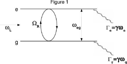
Figure 1: Energy level diagram for two-level system showing decay rates for ground and excited states $\Gamma_{g}$, $\Gamma_{e}$ respectively. The excited and ground state frequency difference is denoted by $\omega_{eg}$. The Rabi oscillation $\Omega_{R}$ is introduced by an external laser frequency $\omega_{L}$.

We now consider the two energy levels ($g$ and $e$) of the damped quantum dot system, the two states are designated as $\psi_{g}$ and $\psi_{e}$ are assumed to be well separated from all other states. The system interacts with a laser of frequency $\omega_{L}$ and $\omega_{a}\equiv\omega_{eg}$ is the resonance frequency (Fig.1). The effect of perturbation produced by the laser can be treated semiclassically using the eigenfunctions of the damped dot $\Psi_{n,l}$ as zeroth order wave function. The perturbed Hamiltonian is partitioned into $H_{0}$ and V, where the unperturbed dot Hamiltonian $H_{0}$ is given by the equation (13) and the perturbation in the dipole approximation: $\overrightarrow{V}=e.rE_{0}\cos(\omega_{L}t)$.

We may now consider the semiclassical perturbation treatment based on the damped wave functions of the damped dot already obtained. The time-dependent Schrodinger equation for the perturbed system is

$$|\dot{\Psi}(r,t)\rangle=-\frac{i}{\hbar}H(r,t)|\Psi(r,t)\rangle$$ (19)

while the solution is (k=e,g)

$$\Psi(r,t)=\sum_{k}C_{k}(t)\psi_{k}(r)e^{-i\omega_{k}^{R}t}e^{-\gamma\omega_{k}^{I}t}$$ (20)

Projecting on to the states $|e\rangle$ and $|g\rangle$ and integrating over spatial coordinates in each case we arrive at the equations governing the time development of the amplitudes $(C_{g}$, and $C_{e})$;

$$i\dot{C_{g}}=C_{g}(t)(\omega_{g}^{R}-i\gamma\omega_{g}^{I})+C_{e}(t)\Omega_{R}\overrightarrow{V}(t)e^{-\gamma\omega_{a}^{I}t}e^{-i\omega_{a}^{R}t}$$ (21)

$$i\dot{C_{e}}=C_{e}(t)(\omega_{e}^{R}-i\gamma\omega_{e}^{I})+C_{g}(t)\Omega_{R}\overrightarrow{V}(t)e^{\gamma\omega_{a}^{I}t}e^{-i\omega_{a}^{R}t}$$ (22)

where the Rabi frequency is defined as $\Omega_{R}=\frac{eE_{0}}{\hbar}\langle e|r|g\rangle$ and the dipole approximation has been used.

Introducing the transformations $\tilde{C_{g}}=[C_{g}e^{(i\omega_{g}^{R}+\gamma\omega_{g}^{I})t}]$ and $\tilde{C_{e}}=[C_{e}e^{(i\omega_{e}^{R}+\gamma\omega_{e}^{I})t}]$

$$i\tilde{C_{g}}=\tilde{C_{e}}\Omega_{R}\overrightarrow{E}(t)e^{(-i\omega_{a}^{R}-\gamma\omega_{a}^{I})t}$$ (23)

$$i\tilde{C_{e}}=\tilde{C_{g}}\Omega_{R}\overrightarrow{E}(t)e^{(i\omega_{a}^{R}+\gamma\omega_{a}^{I})t}$$ (24)

$\overrightarrow{E}(t)=\frac{e^{i\omega_{L}t}+e^{-i\omega_{L}t}}{2}\;;\;\omega_{L}+\omega_{a}=\omega_{+}\;;\;\omega_{L}-\omega_{a}=\ \delta$ detuning frequency
Invoking the rotating wave approximation we get

$$i\dot{\tilde{C_{g}}}=\frac{\Omega_{R}}{2}C_{e}e^{-\gamma\omega_{a}^{I}t}e^{i\delta t}$$ (25)

$$i\dot{\tilde{C_{e}}}=\frac{\Omega_{R}}{2}C_{g}e^{\gamma\omega_{a}^{I}t}e^{-i\delta t}$$ (26)

Equation (26) and (27) can be uncoupled by the standard route, leading to

$$\ddot{\tilde{C_{g}}}-(\gamma\omega_{a}^{I}-i\delta)\dot{\tilde{C_{g}}}+\ \frac{\Omega_{R}^{2}}{4}\tilde{C_{g}}=0$$ (27)

$$\ddot{\tilde{C_{e}}}+(\gamma\omega_{a}^{I}-i\delta)\dot{\tilde{C_{e}}}+\ \frac{\Omega_{R}^{2}}{4}\tilde{C_{e}}=0$$ (28)

Taking the initial condition that $C_{g}(0)=1\;;C_{e}(0)=0$ we get the solutions

$$\tilde{C_{g}} = e^{-\frac{\Delta}{2}t}\left[\cos\frac{\Omega_{Rd}t}{2}+i\frac{\Delta}{\Omega_{Rd}}\sin\frac{\Omega_{Rd}t}{2}\right]$$ (29)

$$\tilde{C_{e}} = e^{\frac{\Delta}{2}t}\;\left[i\frac{\Omega_{R}}{\Omega_{Rd}}\sin\frac{\Omega_{Rd}t}{2}\right]$$ (30)

where $\Delta=\gamma\omega_{a}^{I}-i\delta$   and   $\Omega_{Rd}=\sqrt{\Omega_{R}^{2}-{(\gamma\omega_{a}^{I}-i\delta)}^{2}}$.
Hence,

$$C_{e}=e^{-\gamma(\frac{\omega_{g}^{I}+\omega_{e}^{I}}{2})t}e^{-i\frac{\delta}{2}t}e^{-i\omega_{e}^{R}t}\left[i\frac{\Omega_{R}}{\Omega_{Rd}}\sin\frac{\Omega_{Rd}t}{2}\right]$$ (31)

Hence, the excited state population $P_{e}=|C_{e}|^{2}$ is given by

$$|C_{e}|^{2}=e^{-\gamma(\omega_{g}^{I}+\omega_{e}^{I})t}\left[\frac{{\Omega_{R}}^{2}}{{\Omega_{Rd}}^{2}}\sin^{2}\frac{\Omega_{Rd}t}{2}\right]$$ (32)

The result shows that the contribution of a given state to the evolving wave function $(\Psi)$ of the system at a particular time is given in terms of the damping coefficient and the sum of the energies of the two levels coupled by laser light. The coherent temporal oscillations of the population in the excited state obtained above matches with the experimental observations made by Yu et al Yu02 in Jopsepshon phase qubit. The observed oscillatory behaviour of the decaying amplitude reported by them is successfully explained by our model based on the description of a damped quantum dot by a non-hermitian Hamiltonian in real Coordinates. The probability of being in the state ’k’ (e or g) at any given time is therefore given by $P_{k}(t)=|C_{k}(t)|^{2}$. For the excited state ’e’ Figure 2 shows the nature of the time dependence of $P_{e}$. As expected it is coherently oscillatory and exponentially damped.We note that the equation 33 was earlier developed by Yu et al Yu02 as the asymtotic limit of solution of the appropriate Lioville equation for the density operator under the rotating wave approximation, and used to interpret their experimental observation. We have arrived at the same results based on the non-hermitian Hamiltonian.

IV Conclusion

In summary the proposed model describes correctly the effects of inherent damping in a quantum dot. The amount of dissipating energy in a particular state in a quantum dot is naturally related to the damping coefficient. The decoherence of Rabi oscillations shows that the rate of decoherence is exponentially related not only to the damping coefficient but also to the energy separation between the two levels. Again one interesting point is that the inherent life times of all the different states is predictable assuming that the life time of any one particular state are known from experiment. We also note that the temporal coherent oscillation of population in Josephson junction is correctly explained by the present model.

V Appendix

In atomic units the Hamiltonian of equation (14) reads

$$H=-\frac{1}{2m_{e}}\left(\frac{\partial^{2}}{\partial r^{2}}+\frac{1}{r}\frac{\partial}{\partial r}+\frac{1}{r^{2}}\frac{\partial^{2}}{\partial\phi^{2}}\right)-\frac{i\gamma}{m_{e}}\left(1+r\frac{\partial}{\partial r}\right)-\frac{i\omega_{c}}{2}\left(\frac{\partial}{\partial\phi}\right)+\Omega_{d}^{2}r^{2}$$ (33)

where $\Omega_{d}^{2}=\frac{1}{2}m_{e}\left[\frac{\omega_{c}^{2}}{4}+\frac{\gamma^{2}}{m_{e}^{2}}+\omega_{0}^{2}\right]$.
Substituting, $f(r,\phi)=\frac{e^{(il\phi)}\Psi(r)}{\sqrt{2\pi}}$ and multiplying both sides by $\sqrt{2\pi}e^{-il\phi}r^{\frac{1}{2}}$ leads to radial Schrodinger equation,

$$-\frac{1}{2m_{e}}\left[\frac{d^{2}}{dr^{2}}+\frac{1}{4r^{2}}-\frac{l^{2}}{r^{2}}+\Omega_{d}^{2}r^{2}\right]f(r)+\frac{lw_{c}}{2}-\frac{i\gamma}{m_{e}}\left\{f(r)+rf^{\prime}(r)-\frac{1}{2}f(r)\right\}=Ef(r)$$ (34)

or

$$\left[\frac{d^{2}}{dr^{2}}+(\frac{1}{4}-l^{2})\frac{1}{r^{2}}-\Omega_{d}^{\prime 2}r^{2}-m_{e}\omega_{c}l+2i\gamma(\frac{1}{2}+r\frac{\partial}{\partial r})+2Em_{e}\right]f(r)=0$$ (35)

Where $\Omega_{d}^{\prime 2}=m_{e}^{2}(\frac{\omega_{c}^{2}}{4}+\frac{\gamma^{2}}{m_{e}^{2}}+\omega_{0}^{2})$
Substituting $r=\frac{x}{\sqrt{\Omega_{d}^{\prime}}}$ the radial function $f(r)$ changes to $g(x)$.

$$\left[\frac{d^{2}}{dx^{2}}+\left(\frac{1}{4}-l^{2}\right)\frac{1}{x^{2}}-m_{e}\frac{(\omega_{c}l-2E)}{\Omega_{d}^{\prime}}+2i\frac{\gamma}{\Omega_{d}^{\prime}}\left(\frac{1}{2}+x\frac{d}{dx}\right)+2Em_{e}\right]g(x)=0$$ (36)

Asymptotic analysis leads to
$g(x)=g_{0}(x)V(x)g_{\infty}(x)$ ; $g_{0}(x)=e^{-x^{2}/2}$, $g_{\infty}(x)=x^{\frac{1}{2}+|l|}$
$g(x)=e^{-x^{2}/2}V(x)x^{\frac{1}{2}+|l|}$.
Where $V(x)=\sum_{j}b_{j}x^{j}$ satisfies laguure series. Again taking $z=x^{2}$ the function $V(x)$ changes to function q(z), such that $q(z)=\sum_{k}a_{k}z^{k}$ satisfy the Laguure series.

$$[z\frac{d^{2}}{dz^{2}}+(l+1-z)\frac{d}{dz}-\{\frac{l+1}{2}+m_{e}\frac{(\omega_{c}l-2E)}{4\Omega_{d}^{\prime}}\}$$

$$+2i\frac{\gamma}{4}(1++2z\frac{d}{dz}+l-z)]q(z)=0$$ (37)

where E is complex $(=E_{R}-i\Gamma)$. The Lageurre series satisfies equation (36). Accordingly the total wave function reads

$$\psi_{n,l}(r,\phi)=\frac{C}{2\sqrt{\pi}}e^{i\phi}e^{-\frac{\Omega_{d}^{2}r^{2}}{2}}r^{l}\sum_{0}^{n}b^{n}r^{2n}$$ (38)

VI Acknowledgement

M. Mukhopadhyay would like to thank the CSIR of Goverment of India, New Delhi for the award senior research fellowship. S.P. Bhattacharyya thanks the DST for a generous research grant.

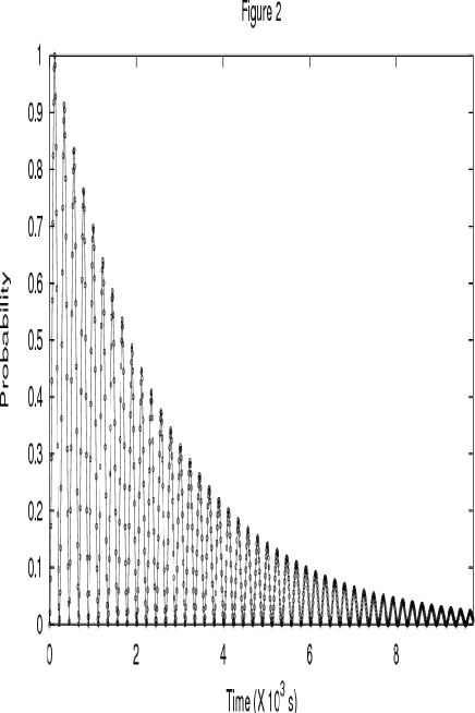
Figure 2: A plot of total population of the excited states versus real time (in a.u) with $m_{e}=$1 a.u., $\omega_{c}=10^{-3}$ a.u., $\omega_{0}=$0.0141 a.u., $\Omega_{R}=0.01$ a.u., $(\omega_{g}+\omega_{e})=0.04$ a.u. and $\gamma=0.0001$ a.u.

References

• (1) I. I. Rabi, Phys. Rev. 51 (1937) 652.
• (2) M. O. Scully, M. S. Zubairy, Quantum Optics. Cambridge University Press, Cambridge,1997.
• (3) Yu. A. Pashkin T. Yamamoto O. Astafiev, Y. Nakamura D. V. Averin, J. S. Tsai, Nature. 421 (2003) 823.
• (4) A. Wallraff, D. I. Schuster, A. Blais, L. Frunzio, R. S. Huang, J. Majer, S. Kumar, S. M. Girvin, R. J. Schoelkofpt, Nature. 431 (2004) 162.
• (5) D. Vion A. Assime, A.Cottet, P.joyez H. Pothier, C. Urbina, D. Esteve, M. H. Dovert, Science. 296 (2002) 886.
• (6) D. O’Brien, S. P. Hegarty, G. Huyet, A. V. Uskov, Optics Letters. 29 (2007) 1072.
• (7) M. Ghosh, R. K. Hazra, S. P. Bhattacharyya, J. Theo. Comp. Chem. 5 (2006) 25.
• (8) V. S. C. M. Rao, S. Hughes, Phys. Rev. Lett. 99 (2007) 193901.
• (9) R. K. Hazra, M. Ghosh, S. P. Bhattacharyya, Chem. Phys. 333 (2007) 18.
• (10) D. P. Fussell, M. M. Dignam, Phys. Rev. A 76 (2007) 053801.
• (11) A. Wallraff, D. I. Schuster, A. Blais, L. Frunzio, J. Majer, M.H. Devoret, S. M. Girvin, R. J. Schoelkopf, Phys. Rev. Lett. 95 (2005) 060501.
• (12) J. M. Martinis, S. Nam, J. Aumentado, Phys. Rev. Lett. 89 (2002) 117901.
• (13) A. Schulzgen, R. Binder, M. E. Donovan, M. Lindberg, K. Wundke, H.M. Gibbs, G. Khitrova, N. Peyghambarian. Phys. Rev. Lett. 82 (1999) 2346.
• (14) T. H. Stievater, X. Li, D. Gammon, D. Park, C. Piermarocchi, L. J. Sham, Phys. Rev. Lett. 87 (2001) 13363.
• (15) A. Zrenner, E.Beham, S.Stufler, F.Findeis, M.Biehler, G.Abstreiter, Nature. 418 (2002) 612.
• (16) N. Kosugi, S. Matsuo, K. Konno, N. Hatakenaka, Phys. Rev. B. 72 (2005) 172509.
• (17) J. M. Villas-Boas, S. E. Ulloa, A. O. Govorov, Phys. Rev. Lett. 94 (2005) 057404.
• (18) Y. Yu, S. Han, Xi. Chu, S. I. chu, Z. Wang, Science. 296 (2002) 889.
• (19) H. Goldstein, Classical Mechanics. 2nd ed. Narosa Publishing House, New Delhi, 2001.
• (20) J.R. Ray, Am. J. Phys. 47 (1979) 626.
• (21) F. Riewe, Phys. Rev. E. 53 (1996) 1890.
• (22) H. Dekker, Phys. Rev. A. 16 (1977) 2126.
• (23) H. Dekker, Phys.Rep. 80 (1981) 1.
• (24) E. G. Harris, Phys. Rev. A. 42 (1990) 3685.
• (25) D. C. Latimer, J. Phys. A: Math. Gen. 38 (2005) 2021.
• (26) V. K. Chandrasekar, M. Stenthilvelan, M. Lakshmanan, J. Math. Phys. 48 (2007) 032701.
• (27) H. Dekker, Z. Physik B. 21 (1975) 295.
• (28) M.S. Wartak, J. Phys. A. Math. Gen. 22 (1989) 361.
• (29) M. Razavy, Z. Physik B. 26 (1977) 201.
• (30) S.Pal, Phys. Rev. A. 39 (1989) 3825.
• (31) V. Fock, Phys Z. 47 (1928) 446.
• (32) C. G. Darwin, Proc. Camb. Philos. Soc. 27 (1930) 86.
Refer to caption