Thermo-dynamic and chemical properties of the Intra-Cluster Medium

Abstract

Aims. We aim to provide constraints on evolutionary scenarios in clusters. One of our main goals is to understand whether, as claimed by some, the cool core/non-cool core division is established once and for all during the early history of a cluster.

Methods. We employ a sample of $\simeq$ 60 objects to classify clusters according to different properties: we characterize cluster cores in terms of their thermo-dynamic and chemical properties and clusters as a whole in terms of their dynamical properties.

Results. We find that: I) the vast majority of merging systems feature high entropy cores (HEC); II) objects with lower entropy cores feature more pronounced metallicity peaks than objects with higher entropy cores. We identify a small number of medium (MEC) and high (HEC) entropy core systems which, unlike most other such objects, feature a large central metallicity. The majority of these outliers are mergers, i.e. systems far from their equilibrium configuration.

Conclusions. We surmise that medium (MEC) and high (HEC) entropy core systems with a large central metallicity recently evolved from low entropy core (LEC) clusters that have experienced a heating event associated to AGN or merger activity.

1 Introduction

The classification of objects is an important step in the construction of viable physical models. This is particularly true for disciplines like astrophysics where, due to the impossibility of performing measurements under a set of rigorously controlled conditions, evolutionary schemes are inferred primarily by comparing properties observed in different objects. Galaxy clusters are no exception to this rule, as for other astrophysical sources, much of the early work has concentrated on establishing a taxonomical framework. In the optical band classification schemes are based on the richness (Abell, 1958; Zwicky et al., 1968) and on the morphological properties which have been found to correlate with the dynamical state of the systems (Abell, 1965, 1975). In X-rays, classification attempts are generally focused on core properties for the rather obvious reason that cores are the regions more easily accessible to observations. Most workers concentrate on defining indicators discriminating between cool core (hereafter CC) and non-cool core (hereafter NCC) systems; these indicators are typically based on estimates of the intensity of the surface brightness peak (Vikhlinin et al., 2007), the temperature (e.g. Sanderson et al., 2006), the cooling time (e.g. Baldi et al., 2007) or the entropy (e.g. Cavagnolo et al., 2009) of the central regions of clusters. There have been attempts to derive dynamical properties of cluster ensembles from X-rays, the best known example is perhaps that of the power-ratios technique (Buote & Tsai, 1995, 1996). Comparison of core with morphological properties, as identified with the power-ratios technique, shows that more disturbed systems tend to have less defined cores (Buote & Tsai, 1996; Bauer et al., 2005). One should however keep in mind that the characterization of the degree of relaxation of clusters through X-ray morphology is limited by projection effects (e.g. Jeltema et al., 2008) and that the limited amount of information available at large cluster radii, beyond $\simeq 0.2R_{180}$, provides a further complication. There have been some attempts to compare dynamical and core properties on individual objects (e.g. A2034, Kempner et al., 2003), sometimes using information from different energy bands (e.g. A1644, Reiprich et al., 2004).

Classification schemes based on chemical properties of clusters have enjoyed considerably less attention. We have known for some time now that CC clusters, formerly known as cooling-flow clusters, feature significant central abundance excesses (De Grandi & Molendi, 2001) and that the amount of iron associated with these excesses is consistent with being produced from the BCG galaxy invariably found at the center of CC systems (De Grandi et al., 2004). Interestingly, there has been no attempt so far to classify clusters by simultaneously making use of thermo-dynamical and chemical properties. In this paper we employ a medium size sample, $\simeq$ 60 objects, to address the issue of cluster classification from various angles, more specifically we will: 1) define an entropy indicator to classify cluster cores with respect to outer regions; 2) provide a dynamical classification based on radio, optical and X-ray properties; 3) compare core and dynamical properties; 4) compare, for the first time, the entropy based classification with a chemical classification. As we shall see, our classification work will allow us to gain considerable insight in how cluster dynamical, thermo-dynamical and chemical properties relate to each other. Another interesting result that will emerge from our analysis is the relevance of outliers, i.e. objects that fall outside of the distributions defined by the majority of systems, in constraining the evolutionary processes that shape galaxy clusters.

The breakdown of the paper is the following. In Sects. 2 and 3 we describe respectively the sample selection and the data analysis. In Sect. 4 we provide an account of how our entropy and cooling time indicators have been constructed. In Sect. 5 we describe two classification schemes based respectively on core and dynamical properties while in Sect. 6 we compare them with the entropy based classification scheme defined in Sect. 4. In Sect. 7 we define a classification scheme based on chemical properties and compare it to the other classification schemes discussed in the paper. Finally in Sect. 8 we summarize our main findings.

Quoted confidence intervals are 68% for one interesting parameter (i.e. $\Delta\chi^{2}$ = 1), unless otherwise stated. All results assume a $\Lambda$CDM cosmology with $\Omega_{\mathrm{m}}=0.3$, $\Omega_{\Lambda}=0.7$, and $H_{0}$ = 70 km s^-1 Mpc^-1.

2 The sample

Starting from the XMM-Newton archive we selected a sample of hot clusters ($kT>3$ keV). The redshift spans between 0.03 and 0.25 and the galactic latitude is greater than 20^∘. Among those clusters satisfying the above selection criteria, we retrieved all observations performed before March 2005 (when the CCD6 of EPIC MOS1 was switched off) and available by the end of May 2007. In Table LABEL:tab:_sample we list the observations of all clusters we analyzed and report cluster physical properties (e.g. redshift and temperature) and observational details (e.g. total exposure time and filter). The redshift value (from optical measurements) is taken from the NASA Extragalactic Database; $kT_{\mathrm{OUT}}$ is derived from our analysis (see Sect. 3.2). Observations are performed using THIN1 or MEDIUM filters. We excluded from the sample observations that are badly affected by soft proton flares, so that the total (i.e. MOS1+MOS2+pn) exposure time for all observations is at least 20 ks. We also excluded observations of extremely disturbed clusters for which it was impossible to define a center; for what concerns double clusters, we analyzed only the brighter of the two subunits. The total number of objects surviving our selection procedures is 59, about half of our objects are local, $0.03<z<0.1$, while the other half is located at intermediate redshifts, $0.1<z<0.25$.

Although not complete, we have reason to believe that our sample is fairly representative of the cluster population as a whole. Indeed objects at $z>0.1$ are extracted by applying a redshift cut at $z=0.25$ from the sample analyzed in Leccardi & Molendi (2008a, b), which we showed to be unaffected by substantial biases (Leccardi & Molendi, 2008b). Similarly the low redshift half of our subsample is extracted from the Edge et al. (1990) flux limited sample by applying neutral cuts such as throwing away observations that are badly affected by soft proton flares. The only selection introducing a certain amount of bias is the one against extremely disturbed clusters for which it was impossible to define a center. We note that only 4 systems were excluded in this manner and that they will be reintroduced in a subsequent paper (Rossetti & Molendi, 2009) where we will make use of the 2D information provided by X-ray maps.

3 Data analysis

In this section we provide some information on the data analysis, a more thorough description may be found in Leccardi & Molendi (2008a) and Leccardi & Molendi (2008b). Here we recall some general issues and highlight a few differences between the analysis performed in this paper and the one conducted in our previous works.

3.1 Event file production

Observation data files (ODF) were retrieved from the XMM-Newton archive and subject to standard processed with the Science Analysis System (SAS) v7.0. The soft proton cleaning was performed using a double filtering process, first in a hard (10-12 keV) and then in a soft (2-5 keV) energy range. The event files were filtered according to PATTERN and FLAG criteria. Bright point-like sources were detected, using a procedure based on the SAS task edetect_chain, and excluded from the event file (see Leccardi & Molendi 2008b for details).

The $R_{\mathrm{SB}}$ indicator, i.e. the ratio between surface-brightness calculated inside and outside the field of view (see Eq. 1 in Leccardi & Molendi 2008b), allowed us to exclude extremely polluted observations and to quantify the quiescent soft proton (QSP) component surviving the double filtering process. Since local clusters fill the whole EPIC field of view, contrary to what we did in Leccardi & Molendi (2008b), we measured $R_{\mathrm{SB}}$ above 9 keV where EPIC effective areas rapidly decrease. We excluded all clusters for which the mean $R_{\mathrm{SB}}$ for the two MOS is greater than 2.0. The threshold is higher than that chosen in Leccardi & Molendi (2008b) because the aim of this work is the analysis of the central regions, where the sensitivity to background variations is not as large as in the outskirts.

3.2 Spectral analysis

To investigate cluster properties in the central regions, we accumulated spectra in two regions: the inner region is a circle of radius 0.05 $R_{180}$ and the outer region an annulus with bounding radii 0.05-0.20 $R_{180}$ (the outer radius of the latter region is limited by the apparent size of the nearest clusters). Both IN and OUT regions are centered on the X-ray emission peak. We recall that $R_{180}$ is the radius within which the mean density is 180 times the critical density and that it has been computed as in Leccardi & Molendi (2008b). Since, as discussed in Sect. 4, $R_{180}$ is itself computed from the temperature measured in the OUT region we have iterated the process until it converged to stable values of $R_{180}$, the first guess for $R_{180}$ was computed using temperatures from Leccardi & Molendi (2008b) and the literature.

For each EPIC instrument and each region, we generated an effective area (ARF), and for each observation we generated redistribution functions (RMF) for MOS1, MOS2, and pn.

Spectra accumulated in the central regions of clusters have almost always high statistical quality; therefore, the complicated procedures we developed for dealing with the background in the outer regions (see Appendices of Leccardi & Molendi 2008b) are not strictly necessary and also EPIC pn data have been used. For all three detectors (namely MOS1, MOS2, and pn), channels were assembled in order to have at least 25 counts for each group, as commonly done when using the $\chi^{2}$ statistic. We merged nine blank-field observations to accumulate background spectra. For each cluster observation, we calculated the count rate ratio, $Q$, between source and background observations above 9 keV in an external ring (10^′–12^′) of the field of view. We scaled the background spectrum by $Q$ and, for each region, subtracted it from the corresponding spectrum from cluster observation. This rough rescaling accounts for possible temporal variations of the instrumental background dominating at high energies without introducing substantial distortions to the source spectrum in the soft energy band where cosmic background components are more important and the source outshines the background by more than one order of magnitude.

The spectral fitting was performed in the 0.5-10.0 keV energy band using the $\chi^{2}$ statistic, with an absorbed thermal model (WABS*MEKAL in XSPEC v11.3). We fit spectra leaving temperature and normalization free to vary. The metallicity was constrained between $\pm 5\;Z_{\odot}$ (see the discussion in Appendix A of Leccardi & Molendi 2008a). The redshift was constrained between $\pm$5% of the optical measurement, and the equivalent hydrogen column density along the line of sight, $N_{\mathrm{H}}$, was fixed to the 21 cm measurement (Dickey & Lockman, 1990). Finally, for each quantity we computed the average over the three (MOS1, MOS2, pn) values and derived the projected emission measure, $E\!M$, as the ratio between the normalization and the area of the region expressed in square arcminutes.

4 Defining interesting quantities

To characterize temperature and emission measure gradients, we need to compare the central to a global value for such quantities; however, for local clusters it was only possible to perform reliable measurements out to a small ($\approx$ 20%) fraction of $R_{180}$. As a temperature reference, we used $kT_{\mathrm{OUT}}$ (see Sect. 3.2), which is found to be a good proxy for the global temperature from Fig. 4 of Leccardi & Molendi (2008b).

Figure 1: Self-similar scaled emission measure profiles for the intermediate-redshift sample presented in Leccardi & Molendi (2008a, b). The radius is in units of $R_{180}$ and the emission measure is scaled by $E\!M_{\mathrm{SSS}}$ (see Eq. 3).

A reference value for the emission measure should be measured at $\approx$ 0.4 $R_{180}$, where profiles show a remarkable degree of similarity (see Fig. 1). We have considered two different proxies for the emission measure at large radii finding that one of them, namely the emission measure calculated in the outer region, $E\!M_{\mathrm{OUT}}$, does somewhat better than the other. We have adopted $E\!M_{\mathrm{OUT}}$ as a proxy for the emission measure at large radii; the interested reader may find a detailed analysis of how well $E\!M_{0}$ and the other proxy approximate the emission measure at large radii in App. A. For the less technically minded readers suffice it to say that $E\!M_{0}$ reproduces the emission measure around 0.4 $R_{180}$ to better than 20%.

Figure 2: Comparison of temperature and emission measure ratios for all clusters. The dashed curves indicate the regions of the plot where the pseudo-entropy ratio, $\sigma$, defined in Eq.(1), is constant; clusters with the strongest pseudo-entropy variations populate the bottom-right corner. Open and filled circles indicate local (i.e. $z\leavevmode\nobreak\ <$ 0.1) and distant (i.e. $z>0.1$) clusters respectively.

In Fig. 2 we compare the temperature ratio, $T_{\mathrm{IN}}/T_{\mathrm{OUT}}$, with the emission measure ratio, $E\!M_{\mathrm{IN}}/E\!M_{\mathrm{OUT}}$. As expected, there is a clear, but quite scattered, correlation: more precisely, the stronger the emission measure peak, the stronger the temperature drop. A key thermo-dynamic observable in describing clusters is the entropy (e.g. Ponman et al., 2003; Voit, 2005; Pratt et al., 2006), which is commonly defined as: $S\equiv T_{X}\times n_{e}^{-2/3}$, where $T_{X}$ and $n_{e}$ are the deprojected temperature and electron density. In the literature (e.g. Rossetti et al., 2007), it is common to define a pseudo-entropy from projected quantities as: $s\equiv T\times E\!M^{-1/3}$. Since we are interested in comparing core with cluster properties we use our emission measure and temperature ratios to define a pseudo-entropy ratio,

$$\sigma\equiv(T_{\mathrm{IN}}/T_{\mathrm{OUT}})\times(E\!M_{\mathrm{IN}}/E\!M_{\mathrm{OUT}})^{-1/3}.$$ (1)

The pseudo-entropy ratio has been found to be well correlated with the entropy ratio, which is computed using deprojected quantities (see Rossetti & Molendi 2009 for a detailed comparison). In Fig. 2 the dashed curves indicate the regions where $\sigma$ is constant; clusters with the strongest variations (i.e. lower ratios) of pseudo-entropy fill the bottom-right corner and are usually known as cool core clusters (see Sects. 5 and 6 for a detailed discussion). Values of the pseudo-entropy ratio for all objects in our sample are reported in Table LABEL:tab:_sigma_z.

The central cooling time is another quantity largely used in the literature (e.g. Peres et al., 1998) to estimate the degree of relaxation of clusters. As done for the entropy, we defined a pseudo-cooling-time, $t_{pc}\equiv T^{1/2}\times E\!M^{-1/2}$, and a pseudo-cooling-time ratio,

$$\tau\equiv(T_{\mathrm{IN}}/T_{\mathrm{OUT}})^{1/2}\times(E\!M_{\mathrm{IN}}/E\!M_{\mathrm{OUT}})^{-1/2}.$$ (2)

When ordering clusters according to $\tau$, we find essentially the same results as when using $\sigma$.

An interesting property of our pseudo-entropy ratio is that it can be constructed from data of moderate statistical quality such as serendipitous observations of clusters in deep XMM-Newton and Chandra observations. In Sect. 6.1 we will employ $\sigma$ to divide clusters into 3 broad categories namely: low entropy core (LEC), medium entropy core (MEC) and high entropy core (HEC) systems. Before we proceed with our entropy based classification we must first consider other classification schemes based, at least in part, on different cluster properties.

5 Alternative classification schemes

We wish to provide alternative classification schemes with which to compare our entropy based scheme. More specifically we wish to compare with: 1) the traditional cool core/non-cool core classification; 2) a classification scheme based on dynamical properties. To avoid circularity, we want the alternative classification schemes to be as independent as possible from our measurements. Therefore, for what concerns the cool core/non cool core classification, we rely on how astronomers have classified these clusters in the literature and not on our own data. More specifically, we divide objects in 3 classes: cool cores (CC), intermediate systems (INT) and non-cool cores (NCC). We classify as CC those systems for which we find evidence in the literature of a temperature decrement and a peaked surface brightness profile. NCC are those that possess neither of the above properties, while INT systems are those that possess one or the other or alternatively both but not as well developed as in full blown cool core systems. We refrain from providing a more quantitative classification for two main reasons: 1) this would be rather difficult to derive from the literature, indeed different authors make use of somewhat different criteria and certainly do not analyze data in a homogenous fashion; 2) our own entropy classification, as we shall see in Sect. 6.1, is best understood as a more quantitative classification scheme along these very lines.

As far as the dynamical classification is concerned we divide object in 2 classes: mergers (MRG), and systems for which we do not find evidence of a merger (NOM). We consider evidence for substantial cluster-wide interaction leading to a merger classification the following phenomena: 1) cluster wide diffuse radio emission such as radio haloes and relics; 2) multi-peaked velocity distribution from optical spectroscopy; or evidence of substructure from the combination of optical spectroscopy and photometry; or evidence for multiple mass peaks from lensing analysis; 3) significant irregularities observed in X-rays both in morphology and temperature maps. The lack of diffuse radio emission or of multi-peaked velocity distribution from optical spectroscopy is in itself insufficient to classify an object as relaxed. Similarly the absence of significant substructure on cluster wide scales in X-ray images is not in itself proof that substructure does not exist or that the system under scrutiny is relaxed. For these reason it is rather difficult to classify a system as relaxed, what we can ascertain is that some systems lack evidence of merger activity. Consequently we classify all objects for which we do not have evidence for merging as “no observed merging” (NOM) systems. We reiterate that a NOM system is not necessarily a relaxed system but rather a system for which we do not have evidence of merging activity, in the sense described previously in this paragraph.

In Table LABEL:tab:_classif we provide results from our classification work. Columns 2 and 3 refer to radio emission, in the first column we indicate with “H” clusters with radio haloes, with “N” clusters without radio haloes, with “?” clusters with tentative radio haloes, with “M” clusters with mini-radio haloes and with “R” clusters with radio relics. Column 3 provides references for column 2. Columns 4 and 5 refer to optical emission, we indicate with “Y” clusters with substructure in the forms described above, with “N” clusters without and with “?” uncertain cases. Column 5 provides references for column 4. Columns 6 and 7 refer to X-ray emission, in column 6 we indicate with “CC” clusters which have been identified as cool core (or cooling flow) systems; with “NCC” clusters that have been identified as non-cool core (or non-cooling flow) systems; with “INT” clusters with intermediate cores and with “MRG” clusters identified as mergers. Column 7 provides references for column 6. In Column 9 we provide our core based classification and in column 10 our dynamical classification. For all objects where a classification cannot be desumed directly from information in columns 2 to 7 we provide a note explaining how the classification was derived. In column 8 we indicate those objects for which we provide a note with “Y” and those for which we do not with “N”.

As far as the core classification is concerned, we classify 24 systems as CC, 25 as NCC and 10 as INT. As far as the dynamical classification is concerned we classify 19 objects as MRG and 40 as NOM.

5.1 Notes on individual objects

5.1.1 A4038

Core Classification

Analysis of Chandra data provides a central cooling time of 1.3 Gyr (Sun et al., 2007) and a flat temperature profile (Sanderson et al., 2006), moreover inspection of Chandra and XMM-Newton images show evidence of an irregular core. This system clearly does not host a full blown cool core, we classify it as intermediate.

Dynamical Classification

Diffuse radio emission has been reported for this source (Slee & Roy, 1998; Slee et al., 2001), although the emission is located at the center of the cluster, its appearance is more similar to that of a radio relic than to a radio halo: it is most likely a remnant associated to the radio galaxy observed in this system. Optical observations (Burgett et al., 2004) provide controversial evidence for substructure on large scales. The evidence pointing to a merger are in our opinion insufficient, we choose to classify this object as NOM.

5.1.2 A3571

Core Classification

Analysis of Chandra data provides a central cooling time of 1.3 Gyr (Sun et al., 2007), however there is no evidence for a temperature decrement in the core (Sakelliou & Ponman, 2006). This system does not host a full blown cool core, we classify it as INT.

Dynamical Classification

On the basis of the multi-wavelength properties of the A3571 cluster complex, Venturi et al. (2002) propose that A3571 is a very advanced merger, and explain the radio properties derived from their study in the light of this hypothesis. We deem the evidence collected by Venturi et al. (2002) insufficient to classify A3571 as a merger and conservatively catalog it as NOM.

5.1.3 A1650

Core Classification

Analysis of Chandra data, readily available through the ACCEPT archive (Cavagnolo et al., 2009), show this object to be of an intermediate nature possessing many of the traits typical of cool cores such as an abundance excess and a temperature drop, albeit with a relatively high core entropy $\simeq$ 40 keV cm². Donahue et al. (2005) define A1650 as a radio quiet cool core speculating that the entropy has been augmented by a recent AGN triggered heating event also responsible for halting the AGN feeding process and ensuing radio manifestations. We classify A1650 as intermediate.

5.1.4 A1689

Core Classification

Analysis of Chandra observations by Cavagnolo et al. (2009) show evidence for a well defined core with a metal abundance excess and a relatively high central entropy of about 80 keV cm². We classify A1689 as an intermediate system.

Dynamical Classification

Optical studies find evidence for two velocity peaks, possibly due to line of sight superposition (Girardi & Mezzetti, 2001). This was later confirmed by Łokas et al. (2006) who performed a detail kinematic study of about 200 galaxies with measured redshifts; Andersson & Madejski (2004) find circumstantial evidence for a merger. We deem the evidence insufficient to classify A1689 as a merger and conservatively catalog it as NOM.

5.1.5 A963

Core Classification

Analysis of Chandra observations by Cavagnolo et al. (2009) show evidence for a well defined core with a modest temperature decrement, a metal abundance excess and a relatively high central entropy of about 60 keV cm². We classify A963 as an intermediate system.

6 Entropy vs. alternative classification schemes

In this section we compare our entropy classification scheme with the core and dynamical classification schemes presented in the previous section.

6.1 Entropy vs. cool core classification scheme

In Fig. 3 we compare our entropy (Sect. 4) and cool core (Sect. 5) classification schemes, we do this by plotting the temperature versus the emission measure ratio as in Fig. 2 with the nuance that we use colors to differentiate objects belonging to different classes, namely we use red for non-cool core (NCC) systems, green for intermediate (INT) systems and blue for cool cores (CC).

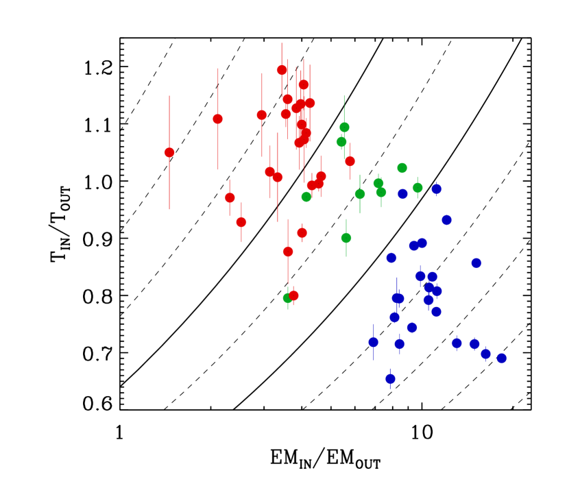
Figure 3: Comparison of temperature and emission measure ratios for all clusters. The dashed and the solid curves indicate the regions of the plot where the pseudo-entropy ratio, $\sigma$, is constant; clusters with the strongest pseudo-entropy variations populate the bottom-right corner. The solid curves indicate the thresholds used to divide clusters in high (HEC), medium (MEC) and low (LEC) entropy core systems. Colors are associated to the cool core classification scheme, namely non-cool cores (NCC) are red, intermediate (INT) are green and cool cores (CC) are blue.

Table 4: Summary of classification schemes.

Scheme	Classification	Acronym
Entropy Ratio	Low Entropy Core	LEC
	Medium Entropy Core	MEC
	High Entropy Core	HEC
Core Properties	Cool Core	CC
	Intermediate	INT
	Non Cool Core	NCC
Dynamic Properties	No Observed Merging	NOM
	Merging System	MRG

Inspection of Fig. 3 shows that, as expected, there is some correlation between the two classifications. More specifically we find that: 1) cool cores have small values of $\sigma$ or, in other words, are characterized by a strong pseudo-entropy gradient; 2) intermediate objects have intermediate entropy gradients; 3) non-cool core, on average, have small entropy gradients. We employ Fig. 3 to divide our objects in 3 broad entropy classes namely: low entropy core (LEC) systems, medium entropy core (MEC) systems and high entropy core (HEC) systems. Given the continuous distribution of objects the precise values of $\sigma$ adopted to separate LEC from MEC and MEC from HEC are of course somewhat arbitrary. One possible criterion is that all INT objects belong to the MEC class. By adopting such a criterion we set the separation between LEC and MEC at $\sigma=0.45$ and the separation between MEC and HEC at $\sigma=0.64$. In Table LABEL:tab:_sigma_z we report the pseudo-entropy ratio and the entropy class for all objects in our sample. To help our readers navigate through the three different classification schemes we have presented, we provide in Table 4 a brief summary including the acronyms that are used extensively in this paper.

Interestingly, while the CC and INT systems separate out quite well in terms of their entropy ratios, the intermediate and non-cool core systems appear to be more mixed up. We find that only 1 CC systems is classified as a MEC and that 7 NCC systems are classified as MEC. The excellent match between LEC systems and cool cores is by no means a surprise, indeed one of the possible definitions of a cool core cluster is that of a system hosting a low entropy core (e.g. Cavagnolo et al., 2009). The agreement should rather be viewed as yet another demonstration of the effectiveness of the $\sigma$ indicator in describing the entropy profiles of clusters. To a lesser extent the same argument may be applied to the MEC vs. INT systems comparison and to the HEC and NCC comparison, however for these systems, particularly for the latter, it becomes progressively more difficult to define the core and its properties. Indeed the more attentive amongst our readers may recall that in Sect. 2 we refrained from including a number of clusters with poorly defined cores in our sample for the very reason that they would be difficult to classify.

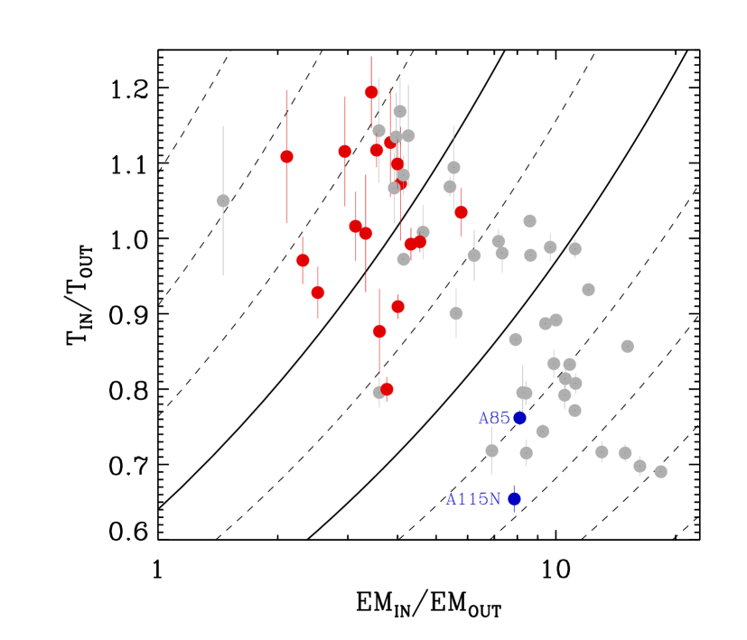
Figure 4: Comparison of temperature and emission measure ratios for all clusters. The dashed and the solid curves indicate the regions of the plot where the pseudo-entropy ratio, $\sigma$, is constant; clusters with the strongest pseudo-entropy variations populate the bottom-right corner. The solid curves indicate the thresholds used to divide clusters in high (HEC), medium (MEC) and low (LEC) entropy core systems. Colors are associated to the dynamics based classification scheme, namely mergers (MRG) are red, with the exception of A115N and A85 which are blue, and systems that do not show evidence for merging (NOM) are gray.

6.2 Entropy vs. dynamical classification scheme

In Fig. 4 we compare our entropy (Sect. 4) and dynamical (Sect. 5) classification schemes, we do this as in Fig. 3 with the difference that the color coding now refers to the dynamical classification, more specifically red for merging (MRG) systems, with the exception of A115N and A85 which are blue, and gray for systems that do not show evidence for merging (NOM). Inspection of Fig. 4 shows that there is some correlation between the two classifications. More specifically we find that: 1) the majority of mergers are HEC systems, a few are classified as MEC systems and 2 are LEC systems; 2) NOM systems are found all over the plot. The result on NOM systems has a trivial explanation, as already discussed in Sect. 5, these are objects for which we do not observe evidence of merging: they will include both systems that are not undergoing a merger and mergers for which we do not have observational evidence of merging activity. A more interesting result is the one on objects identified as mergers. As already noted only a few mergers are MEC and LEC, let us now focus on the 2 MRG with the lowest pseudo-entropy ratios, these are A85 and A115N, which are both LEC systems. A85 and A115N, which are plotted in blue in Fig. 4, are systems where X-ray observations clearly show the presence of two clumps. In both cases the evidence found in the literature supports a scenario where the effects of the merger have not reached the core of the main structure (which is the one for which we computed the entropy ratio), either because the merger is an off-axis merger, A115N (Gutierrez & Krawczynski, 2005), or because it is in an early stage, A85 (Kempner et al., 2002) and A115N (Barrena et al., 2007b). A potential concern for these objects is that, if the sole evidence for the merger not having reached the core were the presence of the core itself, the whole argument would of course be circular and not particularly convincing. We note that if the mergers were in an advanced state we would expect distorted morphology and irregular temperature distribution in the circum-core regions, as well as substantial displacement between X-ray and optical light peaks; this is indeed what is observed in other merging systems (e.g A2256, Sun et al. 2002 and Bourdin & Mazzotta 2008; A3667, Briel et al. 2004 and Vikhlinin et al. 2001) and predicted in simulations (e.g. Rowley et al., 2004; Ricker & Sarazin, 2001). In the cases of A85 no such evidence is found. In the case of A115N, Gutierrez & Krawczynski (2005) find evidence for heating of the region separating the cores, but no indication of supersonic motion, moreover, Barrena et al. (2007b) detect two optical substructures of cluster-type well recognizable in the plane of the sky and roughly coincident with the X-ray peaks thereby favoring a pre-merger scenario. Therefore, in A115N, we have evidence of some form of interaction of minor intensity, that may be explained either in the context of an off-axis merger or in that of an early stage of the merger process.

It is quite interesting that when comparing our core entropy based classification with the dynamical classification, the only 2 mergers to possess a LEC are systems where the effects of the merger have not reached the core. The rather obvious inference, which will be discussed at some length further on in the paper (see Sect. 7.2), is that mergers do have the capability of disrupting low entropy cores. For the time being we note that, if we exclude those interacting systems for which the effects of the merger have not reached the core, we find that MRG systems have pseudo-entropy ratios larger than 0.51. A potential concern is that the same observational evidence may have been used to classify an object as a merger and as a HEC, this would of course provide a rather trivial explanation for the correlation between the two classifications. We note that the presence of a well defined core does not imply that an object may not also show substructure in its surface brightness and temperature maps, indeed A1644 (Reiprich et al., 2004) and A115N (Gutierrez & Krawczynski, 2005) are both good examples of such systems. Moreover only 3 out of the 17 bone-fide mergers, (we have excluded the 2 special cases of A85 and A115N) have been classified as mergers on the basis of their X-ray properties alone; for the other 14 systems there is evidence for a merger from radio and/or optical observations.

In summary the comparison of our entropy and dynamics based classification schemes shows that dynamically active systems tend to have high entropy cores while, with the exception of A85 and A115N where the effects of the mergers have not reached the core, low entropy cores are not found in merging systems.

6.3 Comparison with previous work

Ours is not the first attempt to divide clusters on the basis of their core properties. There have been various works concentrating on somewhat different core properties: Sanderson et al. (2006), for instance, consider the core temperature as discriminator, they define as cool core clusters those systems for which the ratio between average cluster and core temperature exceeds unity at greater than 3$\sigma$ significance. The average cluster temperature is determined from an annulus with bounding radii 0.1-0.2 $R_{500}$ and the core temperature from a circle with radius 0.1 $R_{500}$. The circle is similar to our inner region while the annulus is somewhat smaller than our outer region. While the selection procedure appears to work well for the specific objects in the Sanderson et al. (2006) sample, it has some rather obvious pitfalls, visual inspection of Fig. 3 shows that the range $0.8<T_{\mathrm{IN}}/T_{\mathrm{OUT}}<1.0$ is populated by objects belonging to all 3 entropy classes, i.e. LEC, MEC and HEC, it is only the additional use of the $E\!M_{\mathrm{IN}}/E\!M_{\mathrm{OUT}}$ ratio that allows us to provide a more effective means of separation. As an example of the limitations associated to a classification system based on the temperature decrement alone, we may consider Fig. 4 where we observe that, contrary to what is found when employing the entropy classification scheme, a sizeable fraction of mergers are found in clusters without temperture decrement.

Baldi et al. (2007) use the cooling time, or better the ratio of cooling time to age of the universe at the cluster redshift. As already noted in Sect. 4, a pseudo-cooling-time ratio, $\tau$ defined as in Eq. 2, separates out clusters in much the same way the pseudo-entropy-ratio does. This is illustrated in Fig. 5 where we show the same plot reported in Fig. 3 with the only difference that the dashed lines indicate region of constant $\tau$ rather than $\sigma$.

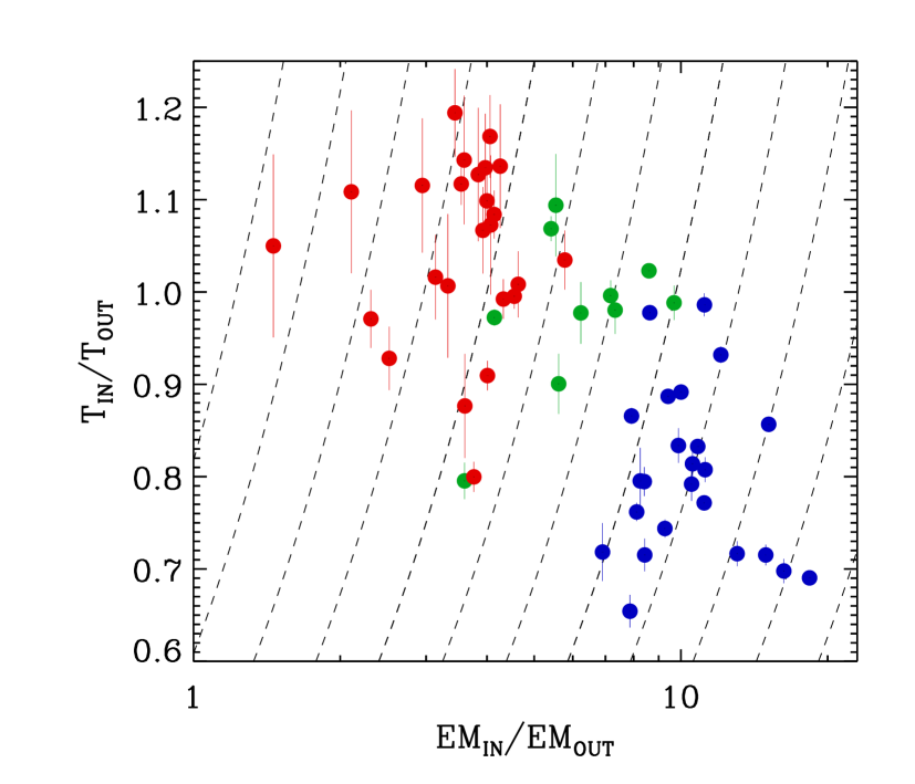
Figure 5: Comparison of temperature and emission measure ratios for all clusters. The dashed curves indicate the regions of the plot where the pseudo-cooling-time ratio, $\tau$, defined in Eq. 2, is constant; clusters with the strongest pseudo- cooling-time variations populate the bottom-right corner. Colors are associated to the cool core classification scheme, namely non-cool core (NCC) are red, intermediate (INT) are green and cool cores (CC) are blue.

Other authors have compared a core based classification with a dynamics based classification. McCarthy et al. (2004) divide objects in cooling flow and non-cooling flow depending on the presence or absence of a temperature gradient in their cores, this is essentially the same classification adopted by Sanderson et al. (2006), they also provide a dynamical classification dividing their objects in relaxed and non-relaxed on the basis of the presence or absence of large scale (a few hundred kpc) substructure in the X-ray images, presumably related to mergers. They find that, of the 33 objects in their sample, 18 are cooling-flow and 15 non-cooling flow. Interestingly, of the 18 cooling flow objects, 12 are classified as relaxed and 6 as non-relaxed and of the 15 non-cooling flow objects 9 are non-relaxed and 6 are relaxed. The presence of a sizable number of non-relaxed cooling flow systems and of relaxed non-cooling flow systems is considered as evidence for a different origin of cooling flows and the relaxed/non-relaxed state in clusters. McCarthy et al. (2004) propose a scenario where an object ends up being cooling or non-cooling flow on the basis of the amount of entropy injected in the system, while the relaxed or non-relaxed nature depends on the object having or not having recently experienced a merger. Our own findings appear to be at variance with what has been reported by McCarthy et al. (2004): the objects we classify as mergers, with the exception of systems where the effects of the merger have not reached the core, are all characterized by a high pseudo-entropy ratio. Since 15 of the 33 object in McCarthy’s sample are also found in ours we have compared our results with theirs . For 11 of the 15 objects that are in common, their classification is in agreement with ours, more specifically: 8 objects are classified as cooling flow and relaxed by McCarthy et al. (2004) and as LEC and NOM by ourselves; 2 objects are classified as non-cooling flow and non relaxed by McCarthy et al. (2004) and as non-low entropy systems, either HEC and MEC, and mergers by ourselves; one object, namely A115N, is classified as cooling flow and non-relaxed by McCarthy et al. (2004) and as LEC and MRG by ourselves. For 4 objects their classification appears to differ from ours. More specifically there is one object, namely A1068, which we classify as LEC and non-merging and McCarthy et al. (2004) classify as cooling flow and non-relaxed. McCarthy et al. (2004) refer to a paper by Wise et al. (2004), which indeed provides evidence for substructure in surface brightness, temperature and metal abundance, however all images presented in that paper cover a region of 200 kpc x 200 kpc and therefore include only the cool core. The kind of substructure found in the core of A1068 is akin to that found in many other cool core systems and is generally believed to be associated to the AGN found at the center of these systems and not to a merger. A second object, A85, is classified as LEC and MRG by ourselves and as non-cooling flow and non-relaxed by McCarthy et al. (2004), however the authors do not specify if the core property is referred to the main structure, which is a well known cool core (e.g. Peres et al., 1998) or to the sub-structure which hosts an intermediate core (Kempner et al., 2002), assuming the latter is the case than the difference in core classification is trivial as we refer to the main structure. The last 2 objects, A1413 and A1689, are classified by McCarthy et al. (2004) as non-cooling flow and relaxed while we classify them as MEC and NOM. A first important point is that McCarthy et al. (2004) define as relaxed those objects for which they do not find evidence of large scale irregularities in the X-ray images, which however does not necessarily imply that these objects are indeed relaxed (an example of such relatively rare systems is A401, a cluster with fairly regular X-ray morphology, Sakelliou & Ponman 2004, featuring a small radio halo, Bacchi et al. 2003, and significant structure in X-ray temperature, Sakelliou & Ponman 2004 and Bourdin & Mazzotta 2008). We classify A1413 and A1689 as MEC in our entropy classification system; both these systems possess a well defined core which, however, is not as prominent as the ones typically found in LEC systems. Indeed analysis of Chandra observations of A1413 and A1689 provide evidence for a well defined core with a modest temperature drop in the core (Vikhlinin et al., 2005; Cavagnolo et al., 2009), a metal abundance excess (Vikhlinin et al., 2005; Cavagnolo et al., 2009) and a relatively high central entropy of about 60 keV cm² and 80 keV cm² respectively (Cavagnolo et al., 2009).

In summary by comparing our classification schemes with those provided by McCarthy et al. (2004) we find that, of the 4 objects for which we do not agree, the 3 objects with mixed classifications i.e. mergers with cooling flows (A1068) and relaxed non-cooling flows (A1413 and A1689) cannot be used to support a scenario where the absence or presence of a cooling flow is unrelated to the object having or not having experienced a merger. Indeed the former object is non-relaxed on small scales in much the same way as other cool core systems and for the latter two: I) the lack of evidence for a merger does not necessarily mean that a merger is not present; II) the classification as non-cooling flow is insufficiently accurate, as both these system host well defined intermediate cores.

7 Chemical properties

In this section we compare chemical with thermo-dynamic properties for the objects in our sample. As a first step we discuss metal abundance profiles.

7.1 Metallicity profiles

We have divided our sample in the entropy classes defined in Sect. 6 and produced mean radial metallicity profiles for each entropy class. Metal abundance profiles for individual systems come from Leccardi & Molendi (2008a) for the intermediate redshift subsample and from Rossetti & Molendi (2009) from the low redshift sample.

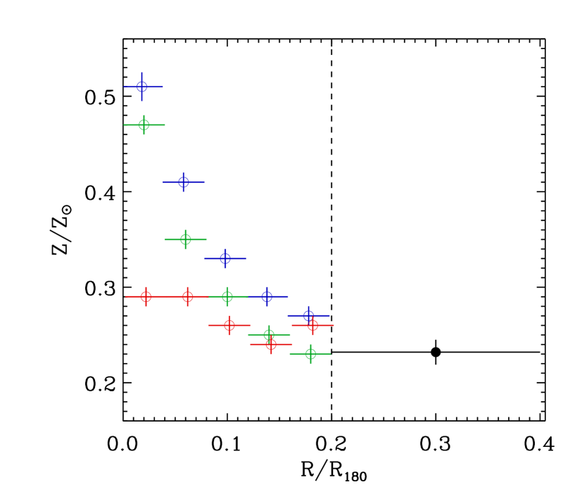
Figure 6: Mean metallicity profiles for LEC (blue circles), MEC (green), and HEC (red) clusters. Abundances are expressed in Anders & Grevesse (1989) solar values. The dashed line indicates 0.2 $R_{180}$, the radius within which profiles are obtained from all clusters, the black data point beyond 0.2 $R_{180}$ is the average value from distant (i.e. $z>0.1$) clusters belonging to all entropy classes.

In Fig. 6 we show the mean profiles for LEC, MEC, and HEC clusters, the binning is in units of $R_{180}$ and was computed as in Leccardi & Molendi (2008a); for each bin the average is calculated by allowing for an intrinsic dispersion. As can be seen in Fig. 6, within 0.1 $R_{180}$, a region typically associated with the core, all profiles show an abundance excess. The excess is strongest for LEC, somewhat weaker for MEC, and weakest for HEC clusters. Interestingly the modest excess observed in HEC clusters is similar to the one obtained from a BeppoSAX sample of non-cool core clusters (De Grandi & Molendi, 2001) dominated by well known merging systems. Between 0.1 and 0.2 $R_{180}$ the profiles for the three classes are roughly consistent with one another and, at least for LEC and MEC systems, show a significant excess with respect to the mean value measured in the outskirts. Between 0.2 and 0.4 $R_{180}$, where we have data for the intermediate-redshift sample only, the three profiles are consistent with being flat and equal with each other. We therefore plot the abundance averaged over all 3 entropy classes, which turns out to be $0.23\pm 0.01\;Z_{\odot}$, and in good agreement with the value obtained by De Grandi & Molendi (2001) for a local sample of relaxed clusters observed with BeppoSAX. As already discussed in Sect. 4, the precise choice of pseudo entropy ratio values used to divide objects in the three entropy classes is rather arbitrary; by experimenting with slightly different values we find that, while the details of the profiles may change somewhat as borderline objects are shifted from one class to another, the qualitative description provided above remains valid.

An important point is that the abundance measures in the outer region are not only consistent with being flat but also appear to be independent of the entropy class (HEC, MEC or LEC) or of the dynamical class (MRG or NOM) of the object. Moreover the mass of ICM enclosed within 0.2 and 0.4 $R_{180}$ is about two times that contained within 0.2 $R_{180}$ and, according to De Grandi et al. (2004), the Fe mass in the abundance excess of CC clusters is roughly 10% of the Fe mass integrated out to 0.25 $R_{180}$. It follows that estimates of how the global metal abundance varies with respect to other quantities are best performed by making measures in the 0.2-0.4 $R_{180}$ range. An example, which we shall not discuss further, is the often quoted anti-correlation between metal abundance and temperature (Baumgartner et al., 2005; Balestra et al., 2007). Another example is the measure of the evolution of the global metal abundance with cosmic time. Current estimates (Balestra et al., 2007; Maughan et al., 2008) are performed at small radii where the presence of an abundance excess, more pronounced in some systems than in others, poses a major obstacle. Both Balestra et al. (2007) and Maughan et al. (2008) are aware of these difficulties and confront them either by gauging how the mix of cool cores and non cool cores might affect the observed evolution in the iron abundance (Balestra et al., 2007), or by excising the innermost region (0.15 $R_{500}$) from their spectra (Maughan et al., 2008). A more robust approach would be to restrict measures to the 0.2-0.4 $R_{180}$ range. In Leccardi & Molendi (2008a) we showed that by adopting the above radial range in the limited redshift interval covered by our data, $0.1<z<0.3$, we could not discriminate between no variation of the abundance with redshift and a variation of the kind described in Balestra et al. (2007). Extension of these kind of measures out to $z\simeq$0.5, while observationally challenging, would allow to discriminate between the two competing alternatives.

7.2 Chemical vs. thermo-dynamic quantities

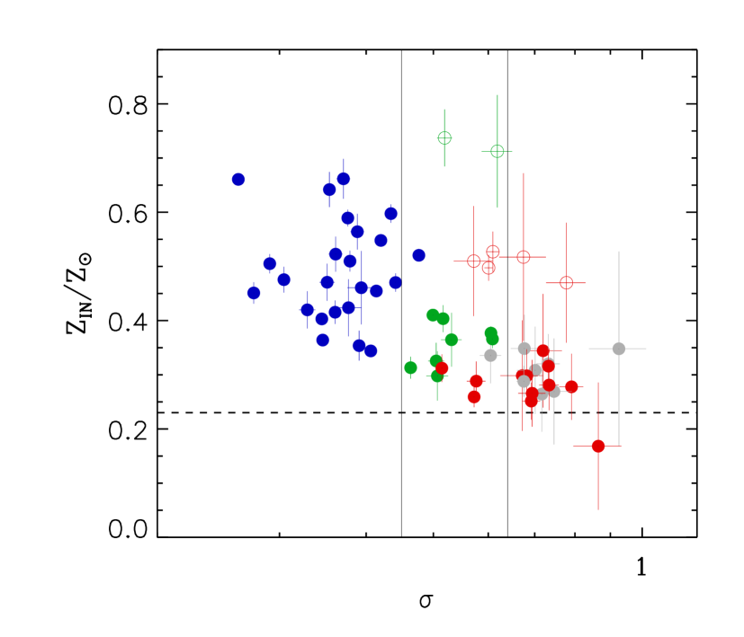
Figure 7: Central metallicity, $Z_{\mathrm{IN}}$, vs. pseudo-entropy ratio, $\sigma$. In blue and green we indicate objects that, within the core classification scheme, are respectively identified as CC and INT systems. In red and grey we indicate objects that, within the dynamical classification scheme, are respectively identified as MRG and NOM. In the few instances where the two classification schemes require different colors, the core scheme takes precedence. Open circles indicate high metallicity MEC and HEC systems. Abundances are expressed in Anders & Grevesse (1989) solar values. The dashed horizontal line at $0.23\;Z_{\odot}$ indicates the mean metallicity in the outer regions of clusters (Leccardi & Molendi, 2008a). The solid vertical lines mark the boundary between the three entropy classes (see Sect. 6.1 for details).

In Fig. 7 we plot the metallicity measured in our inner region, $Z_{\mathrm{IN}}$, vs. the pseudo-entropy ratio, $\sigma$, for all clusters in our sample. Values of $Z_{\mathrm{IN}}$ and $\sigma$ are also reported in Table LABEL:tab:_sigma_z. We find $\sigma$ and $Z_{\mathrm{IN}}$ to have a negative correlation, namely: the stronger the pseudo-entropy gradient, the stronger the metallicity peak. This results tells that, baring a few exceptions that we will discuss later in this section, the metal rich gas in clusters also happens to be the low entropy gas. An important point that we only mention here and that we have discussed in detail elsewhere is the presence of a consistent scatter in the abundance distribution, particularly for LEC systems (De Grandi & Molendi, 2009). The most interesting result is arguably the presence of a few (7) MEC and HEC systems with unusually high metal abundance. Of these high Z systems 4, namely A1644, AS0084, A576 and A3562, have metalicities well above the typical values found for other MEC and HEC systems, while 3, namely A2034, A209 and A1763, suffering from large indetermination in there abundance estimates, show poor statistical evidence of an excess (roughly 2$\sigma$). For A2034, a long Chandra observation (Baldi et al., 2007) provides a somewhat tighter constraint which raises the significance to about 3$\sigma$.

From our classification work (see Sect. 5) we know that a large fraction of these objects, 5/7, are mergers (they are shown in red in Fig. 7). In other words, most of our high metallicity MEC and HEC systems are undergoing a phase of rapid dynamical change. This simple consideration leads to the question of the original equilibrium configuration from which these systems evolved. There are two issues that should be kept in mind when addressing this question. The first is that metals are reliable markers of the ICM, in the sense that, once metals have polluted a given region of a cluster, the timescale over which the same metals will diffuse is comparable, likely longer, than the Hubble time (Sarazin, 1988; Chuzhoy & Nusser, 2003). Thus, for all practical purposes, metals trace the region of the ICM where they have been injected and can be diluted only if the ICM itself undergoes mixing processes. The second is that abundances such as those observed in our metal rich MEC and HEC systems are found in the cores of LEC systems, indeed our own analysis (see Fig. 7) shows that every LEC system has an excess with respect to the metal abundance found in cluster outer regions.

Keeping the above considerations in mind, the most likely explanation is that our high abundance MEC and HEC clusters originate from LEC systems that have undergone substantial heating. While for one of our objects, namely A1644, the relatively modest entropy ratio is not inconsistent with heating from the central AGN, as is observed in other intermediate systems such as A1650 (Donahue et al., 2005), for all other systems the required heating is beyond what can be provided by the central AGN and must come from some other mechanism. Since all but one of the other 6 high metallicity objects show evidence of a merger, it seems reasonable to assume that the heating may indeed be provided by the merger event.

This interpretation however clashes with claims from at least 2 groups conducting cluster simulations. According to Poole et al. (2006, 2008) and Burns et al. (2008), once cool cores form it is extremely difficult to disrupt them. The above authors suggest that the fate of a cluster (LEC or otherwise) is decided early on in its history; if it is subject to an event that raises its entropy than it will likely not develop a cool core and subsequent mergers will be effective in maintaining the high entropy state. Conversely, if a cool core is formed early on, it will be very difficult to disrupt, i.e. subsequent mergers will not destroy the entropy stratification. In our opinion the scenario described in Poole et al. (2006, 2008) and Burns et al. (2008) suffers from two major shortcomings, one on the observational side, the other on the theoretical side. Let us consider the former; if the presence/absence of cool cores is not related to the dynamical state of a cluster one would expect to observe LEC in some merging clusters, and HEC in some relaxed systems. In Sect. 5 we have shown that: 1) having excluded A85 and A115N, where the effects of the merger have not reached the core, for none of the remaining 21 LEC clusters do we find evidence that they are located in a merging system; 2) all our merging systems, baring the afore quoted exceptions of A85 and A115N, are MEC or HEC systems, with the vast majority being HEC (11/17). These findings are at variance with those reported by McCarthy et al. (2004) who do identify a few non-relaxed cooling-flow systems and relaxed non cooling-flow systems. In Sect. 6.3 we have compared our entropy and dynamical classification schemes with those presented in McCarthy et al. (2004) for the 15 objects that are present in both samples finding that, of the 4 cases where our classifications do not agree, 3 likely result from misclassifications by McCarthy et al. (2004), while the fourth probably has a trivial explanation.

The second shortcoming is related to the fact that current simulations cannot reproduce observed cool cores, rather they produce something more akin to traditional cooling flows. Poole et al. (2006, 2008) correct for this by imposing initial conditions in the core so as to reproduce observed cool cores, however merger events run on timescales longer than the cooling time in cores. Indeed, as pointed out in Poole et al. (2006), within 0.5 Gyr, well before the clusters begin interacting significantly, the central entropy profile reverts to the self similar power law shape. Alternatively Burns et al. (2008) strive to reproduce observed cool cores by introducing ad-hoc sub-grid recipes. Thus, if simulations cannot provide a self consistent picture of cool cores, why should we be compelled to trust simulations that tell us that cool cores survive mergers?

Recently Sanderson et al. (2009) have provided observational evidence favoring scenarios where cluster mergers are capable of erasing cool cores. These authors have shown that in a sample of 65 objects, the X-ray/BCG projected offset correlates with the gas density profile. Under the assumption that the offset serves to measure the dynamical state of the cluster, their result implies that the cool core strength progressively diminishes in more dynamically disrupted clusters. Such a trend is expected if cluster mergers are capable of erasing cool cores.

8 Summary

The main results presented in this paper may be summarized as follows.

• We have constructed an indicator of the entropy of the core relative to that of the cluster, the pseudo entropy ratio $\sigma$. Our indicator is robust, in the sense that somewhat different choices of the quantities from which the ratio is computed result in very similar values of $\sigma$. The indicator is also relatively parsimonious, in the sense that it may be constructed from data of moderate statistical quality.

• The classification of clusters based on the entropy indicator improves upon the traditional classification scheme based on the presence or absence of a temperature drop in the core. Conversely classification schemes based on the central cooling time appear to be essentially equivalent to ours.

• A comparison between the entropy based classification scheme and a classification scheme based on dynamical properties shows that the large majority of merging systems are characterized by large entropy ratios. Only 2 of our merging systems feature a low entropy core (LEC) and in both cases we were able to establish, with reasonable certainty, that the effects of the merger have not reached the core. Our findings are at variance with those presented by McCarthy et al. (2004) who do find evidence of non relaxed cooling flow systems and relaxed non-cooling flow systems. We have compared our entropy and dynamical classification schemes with those in McCarthy et al. (2004) for the 15 objects that are common to both samples finding that the 3 cases where our classifications do not agree likely result from misclassifications by McCarthy et al. (2004).

• We find that mean abundance profiles for our 3 entropy classes, namely low entropy core (LEC), medium entropy core MEC, and high entropy core (HEC), may be divided in 3 regions. In the outer region, between 0.2 and 0.4 $R_{180}$, all 3 profiles are consistent with being flat and with one another. In the core region, within 0.1 $R_{180}$, all classes feature an excess with respect to the mean value found in the outer regions. The excess is strongest for LEC, somewhat weaker for MEC, and weakest for HEC clusters. Between 0.1 and 0.2 $R_{180}$ the profiles for the three classes are roughly consistent with one another and, at least for LEC and MEC systems, show a significant excess with respect to the mean value measured in the outskirts.

• We find that objects with stronger pseudo-entropy gradients have more pronounced metallicity peaks. This results tells that, baring a few exceptions, the gas that is more enriched in metals also happens to be the one featuring the lowest entropy.

• We have identified a small number of medium and high entropy core systems with a large central metallicity. The majority of these objects have been classified as mergers, i.e. as systems far from their equilibrium configuration. We surmise that these systems evolved from low entropy core clusters that have experienced a heating event. We have examined simulation based claims that conflict with our conjecture finding they are flawed both on the observational and the theoretical side.

In an upcoming paper (Rossetti & Molendi 2009) we will investigate further the issue of medium and high entropy core systems with a large central abundance; we will do this by performing bi-dimensional analysis of a smaller sample of bright and nearby clusters.

Appendix A

In this Appendix we compare $E\!M_{\mathrm{OUT}}$, the emission measure from the 0.05-0.20 $R_{180}$ ring, with another proxy for the emission measure at large radii, namely the self-similar scaling factor $E\!M_{\mathrm{SSS}}$ which is defined as:

$$E\!M_{\mathrm{SSS}}\equiv\Delta_{\mathrm{z}}^{3/2}\,(1+z)^{9/2}\,(\mathrm{k}T_{\mathrm{OUT}}/10\,\mathrm{keV})^{1/2},$$ (3)

for details about this definition we refer our readers to Arnaud et al. (2002). As a reference value of the emission measure at large radii we employ $E\!M_{0}$, the emission measure calculated in the 0.2-0.4 $R_{180}$ ring. $E\!M_{0}$ is available for the subsample of distant ($z>0.1$) clusters, for which it is possible to measure $E\!M$ out to 0.4 $R_{180}$ (the values of $E\!M_{0}$ are taken from Leccardi & Molendi 2008b). Since we are interested in emission measure ratios, for each distant cluster, we calculated our “ideal” ratio $E\!M_{\mathrm{IN}}/E\!M_{0}$, determined directly from the data, the self-similar scaled ratio $E\!M_{\mathrm{IN}}/E\!M_{\mathrm{SSS}}$, and the standard ratio $E\!M_{\mathrm{IN}}/E\!M_{\mathrm{OUT}}$.

Figure 8: Correlations between various definitions for the $E\!M$ ratios (see text for details). Left panel: self-similar scaled vs. ideal ratios. Right panel: standard vs. ideal ratios. The solid curve is the best fit with a power law. The uncertainties are smaller than the point size. The scatter is 29% and 16% for left and right panels respectively.

In Fig. 8 we compare the self-similar scaled (left panel) and the standard (right panel) ratios to the ideal ratio. For both cases we find a good correlation, but the scatter is smaller (16% vs. 29%) when using the standard ratio. Throughout this paper we make use of $E\!M_{\mathrm{IN}}/E\!M_{\mathrm{OUT}}$, but we emphasize that our results are largely independent of this particular choice. Indeed, the appearance of the plot in Fig. 2 is very similar when using

$$\tilde{\sigma}\equiv(T_{\mathrm{IN}}/T_{\mathrm{OUT}})\times(E\!M_{\mathrm{IN}}/E\!M_{\mathrm{SSS}})^{-1/3},$$ (4)

which differs from $\sigma$ for the use of the self-similar scaling.

Figure 9: Correlation between $\sigma$ and $\tilde{\sigma}$ (see text for definitions) for clusters with $z>0.1$. The solid line shows the best-fit power law; the scatter is $\approx$ 6%.

In Fig. 9 we show the correlation between $\sigma$ and $\tilde{\sigma}$ for the subsample of distant clusters; we find a small, $\approx$ 6%, scatter around the best-fit power law (represented with a solid line); this is another confirmation of the robustness of our entropy indicator.

Table 5: Physical properties and observation details for the 59 clusters of our sample.

Name	$z\mathrm{{}^{a}}$	$kT_{\mathrm{OUT}}\mathrm{{}^{b}}$	Exp. timec	$R_{\mathrm{SB}}\mathrm{{}^{d}}$	Filter
Abell 4038	0.0300	3.0	78.1	1.45	MEDIUM
Abell 2199	0.0301	4.1	38.4	1.14	THIN1
2A 0335+096	0.0349	3.6	230.8	1.02	THIN1
Abell 2052	0.0355	2.9	85.1	0.99	THIN1
Abell 576	0.0390	3.8	42.7	1.54	MEDIUM
Abell 3571	0.0391	6.3	43.5	1.54	MEDIUM
Abell 119	0.0442	6.0	54.1	1.62	THIN1
MKW 03	0.0450	3.3	99.2	1.08	THIN1
Abell 3376	0.0456	3.9	56.4	1.10	MEDIUM
Abell 1644	0.0470	4.2	42.0	1.40	THIN1
Abell 4059	0.0475	4.0	64.9	1.11	THIN1
Abell 3558	0.0480	5.2	126.4	1.00	THICK
Abell 3562	0.0480	4.3	116.6	1.85	THIN1
Triangulum Austr.	0.0510	9.2	27.3	1.15	MEDIUM
Hydra A	0.0538	3.4	52.2	1.59	THIN1
Abell 754	0.0542	8.7	30.8	1.11	MEDIUM
Abell 85	0.0551	5.5	34.6	1.04	MEDIUM
Abell 2319	0.0557	9.2	44.6	1.80	MEDIUM
Abell 3158	0.0597	4.9	54.0	1.58	THIN1
Abell 1795	0.0625	5.4	97.3	1.29	THIN1
Abell 399	0.0720	6.0	27.9	1.84	THIN1
Abell 401	0.0740	7.3	34.7	1.76	MEDIUM
Abell 3112	0.0750	4.3	64.6	1.23	MEDIUM
Abell 2029	0.0773	6.2	30.8	1.17	THIN1
Abell 2255	0.0806	6.2	25.1	1.37	THIN1
Abell 1650	0.0838	5.4	75.0	1.29	MEDIUM
Abell 2597	0.0852	3.5	144.3	1.07	THIN1
Abell S0084	0.1080	3.3	44.8	1.28	THIN1
Abell 2034	0.1130	7.0	27.9	1.16	THIN1
Abell 2051	0.1150	3.8	83.6	1.08	THIN1
Abell 3814	0.1179	3.3	71.2	1.11	THIN1
Abell 2050	0.1183	5.3	77.3	1.13	THIN1
RXCJ1141.4-1216	0.1195	3.8	82.0	1.03	THIN1
Abell 1084	0.1323	3.9	72.4	1.03	THIN1
Abell 1068	0.1375	4.5	56.3	1.09	MEDIUM
Abell 3856	0.1379	6.4	54.6	1.11	THIN1
Abell 3378	0.1410	4.9	58.3	1.07	THIN1
Abell 0022	0.1424	5.7	41.9	1.02	THIN1
Abell 1413	0.1427	6.7	71.7	1.10	THIN1
Abell 2328	0.1470	5.6	71.1	1.07	THIN1
Abell 3364	0.1483	6.7	67.1	1.12	THIN1
Abell 2204	0.1522	8.5	51.2	1.06	MEDIUM
Abell 0907	0.1527	6.1	22.9	1.16	THIN1
Abell 3888	0.1529	8.6	42.8	1.31	THIN1
RXCJ2014.8-2430	0.1612	7.1	64.8	1.05	THIN1
Abell 3404	0.1670	7.1	59.2	1.11	THIN1
Abell 1914	0.1712	8.7	62.9	1.17	THIN1
Abell 2218	0.1756	6.5	117.0	1.17	THIN1
Abell 1689	0.1832	9.2	106.7	1.14	THIN1
Abell 383	0.1871	4.4	82.3	1.33	MEDIUM
Abell 115N	0.1971	5.1	103.2	1.20	MEDIUM
Abell 2163	0.2030	15.5	29.2	1.07	THIN1
Abell 963	0.2060	6.5	69.4	1.19	MEDIUM
Abell 209	0.2060	6.6	49.3	1.19	MEDIUM
Abell 773	0.2170	7.5	45.6	1.16	MEDIUM
Abell 1763	0.2230	7.2	36.3	1.08	MEDIUM
Abell 2390	0.2280	11.2	29.4	1.11	THIN1
Abell 2667	0.2300	7.7	59.9	1.48	MEDIUM
RX J2129.3+0005	0.2350	5.5	102.0	1.21	MEDIUM

• ^a redshift taken from the NASA Extragalactic Database; ^b reference temperature in keV derived from our analysis (see Sect. 3.2); ^c total good exposure time in ks; ^d intensity of residual soft protons (see Sect. 3.1).

Table 6: Pseudo-entropy ratio and metal abundances for the inner region of the 59 objects in our sample.

Name	$\sigma\mathrm{{}^{a}}$	Entropy	$Z_{\mathrm{IN}}/Z_{\odot}\mathrm{{}^{c}}$
		Classif.b
Abell 4038	$0.499\pm 0.004$	MEC	$0.41\pm 0.01$
Abell 2199	$0.414\pm 0.003$	LEC	$0.45\pm 0.01$
2A 0335+096	$0.262\pm 0.001$	LEC	$0.66\pm 0.00$
Abell 2052	$0.420\pm 0.003$	LEC	$0.55\pm 0.01$
Abell 576	$0.609\pm 0.013$	MEC	$0.53\pm 0.04$
Abell 3571	$0.608\pm 0.008$	MEC	$0.37\pm 0.02$
Abell 119	$0.734\pm 0.024$	HEC	$0.28\pm 0.05$
MKW 03	$0.477\pm 0.004$	MEC	$0.52\pm 0.01$
Abell 3376	$0.682\pm 0.025$	HEC	$0.30\pm 0.05$
Abell 1644	$0.519\pm 0.013$	MEC	$0.74\pm 0.05$
Abell 4059	$0.434\pm 0.004$	LEC	$0.60\pm 0.02$
Abell 3558	$0.605\pm 0.006$	MEC	$0.38\pm 0.01$
Abell 3562	$0.601\pm 0.008$	MEC	$0.50\pm 0.02$
Triangulum Austr.	$0.675\pm 0.016$	HEC	$0.29\pm 0.03$
Hydra A	$0.406\pm 0.004$	LEC	$0.34\pm 0.01$
Abell 754	$0.514\pm 0.011$	MEC	$0.31\pm 0.03$
Abell 85	$0.379\pm 0.005$	LEC	$0.51\pm 0.02$
Abell 2319	$0.572\pm 0.010$	MEC	$0.26\pm 0.02$
Abell 3158	$0.733\pm 0.015$	HEC	$0.32\pm 0.03$
Abell 1795	$0.345\pm 0.002$	LEC	$0.40\pm 0.01$
Abell 399	$0.694\pm 0.031$	HEC	$0.27\pm 0.06$
Abell 401	$0.692\pm 0.021$	HEC	$0.25\pm 0.03$
Abell 3112	$0.376\pm 0.004$	LEC	$0.59\pm 0.02$
Abell 2029	$0.441\pm 0.006$	LEC	$0.47\pm 0.02$
Abell 2255	$0.865\pm 0.069$	HEC	$0.17\pm 0.12$
Abell 1650	$0.516\pm 0.009$	MEC	$0.40\pm 0.02$
Abell 2597	$0.346\pm 0.002$	LEC	$0.36\pm 0.01$
Abell S0084	$0.618\pm 0.031$	MEC	$0.71\pm 0.10$
Abell 2034	$0.778\pm 0.051$	HEC	$0.47\pm 0.11$
Abell 2051	$0.746\pm 0.046$	HEC	$0.27\pm 0.10$
Abell 3814	$0.371\pm 0.008$	LEC	$0.66\pm 0.04$
Abell 2050	$0.733\pm 0.028$	HEC	$0.32\pm 0.05$
RXCJ1141.4-1216	$0.354\pm 0.005$	LEC	$0.64\pm 0.03$
Abell 1084	$0.361\pm 0.006$	LEC	$0.42\pm 0.02$
Abell 1068	$0.304\pm 0.006$	LEC	$0.48\pm 0.02$
Abell 3856	$0.605\pm 0.022$	MEC	$0.34\pm 0.05$
Abell 3378	$0.389\pm 0.009$	LEC	$0.56\pm 0.03$
Abell 0022	$0.701\pm 0.041$	HEC	$0.31\pm 0.08$
Abell 1413	$0.505\pm 0.013$	MEC	$0.33\pm 0.03$
Abell 2328	$0.926\pm 0.087$	HEC	$0.35\pm 0.18$
Abell 3364	$0.676\pm 0.030$	HEC	$0.35\pm 0.06$
Abell 2204	$0.290\pm 0.005$	LEC	$0.51\pm 0.02$
Abell 0907	$0.394\pm 0.018$	LEC	$0.46\pm 0.07$
Abell 3888	$0.717\pm 0.037$	HEC	$0.26\pm 0.07$
RXCJ2014.8-2430	$0.275\pm 0.005$	LEC	$0.45\pm 0.02$
Abell 3404	$0.507\pm 0.018$	MEC	$0.30\pm 0.05$
Abell 1914	$0.577\pm 0.018$	MEC	$0.29\pm 0.04$
Abell 2218	$0.791\pm 0.031$	HEC	$0.28\pm 0.06$
Abell 1689	$0.464\pm 0.009$	MEC	$0.31\pm 0.02$
Abell 383	$0.361\pm 0.008$	LEC	$0.52\pm 0.03$
Abell 115N	$0.329\pm 0.009$	LEC	$0.42\pm 0.03$
Abell 2163	$0.720\pm 0.046$	HEC	$0.34\pm 0.10$
Abell 963	$0.572\pm 0.037$	MEC	$0.51\pm 0.10$
Abell 209	$0.531\pm 0.018$	MEC	$0.36\pm 0.05$
Abell 773	$0.672\pm 0.047$	HEC	$0.30\pm 0.10$
Abell 1763	$0.674\pm 0.052$	HEC	$0.52\pm 0.15$
Abell 2390	$0.377\pm 0.016$	LEC	$0.42\pm 0.05$
Abell 2667	$0.351\pm 0.009$	LEC	$0.47\pm 0.03$
RX J2129.3+0005	$0.391\pm 0.008$	LEC	$0.35\pm 0.03$

• ^a pseudo-entropy ratio, see Sect. 4 for details; ^b pseudo entropy class, see Sect. 6.1 for details; ^c metal abundance in central region, see Sect. 7.2 for details.

Table 7: Classification of objects based on radio, optical and X-ray properties.

Name	Ra	R.ref	Ob	O.ref	X-rayc	X-ray ref	Note	Core Cl.	Dyn.Cl.
Abell 4038	H	Sl98,Sl01	?	Bu04	NCC	Sn06	Y	INT	NOM
Abell 2199	-		?	Oe01	CC	Jo02	N	CC	NOM
2A 0335+096	-		-		CC	Ma03	N	CC	NOM
Abell 2052	-		N	Di87,Ma92	CC	Bl03	N	CC	NOM
Abell 576	N	Fe07	-		MRG & NCC	Mo96,Ke04,Du07	N	NCC	MRG
Abell 3571	N	Ve02	-		NCC	Oh06,Sn06,Da08	Y	INT	NOM
Abell 119	N	Mu04	-		MRG & NCC	Sr06,Ro06	N	NCC	MRG
MKW 03	-		-		CC	Ma02,Su07	N	CC	NOM
Abell 3376	R	Ba06	N	Gi97	MRG & NCC	Ro06,Ca09	N	NCC	MRG
Abell 1644	-		N	Tu01	INT	Re04,Du05	N	INT	NOM
Abell 4059	-		-		CC	Ch04,Ca09	N	CC	NOM
Abell 3558	N	Ba98	Y	Ba98	INT	Ro07	N	INT	NOM
Abell 3562	H	Gi05	Y	Ba98	MRG & NCC	Fi04	N	NCC	MRG
Triangulum Austr.	-		-		NCC	Ch07	N	NCC	NOM
Hydra A	-		-		CC	Da01	N	CC	NOM
Abell 754	H	Ka01,Ba03	?	Ro98	MRG & NCC	Kr03,He04	N	NCC	MRG
Abell 85	-		N	Ma92,Br09	MRG & CC	Ke02,Dr05	N	CC	MRG
Abell 2319	H	Fe97,Ca06	Y	Oe95	MRG & NCC	Oh04	N	NCC	MRG
Abell 3158	-		Y	Jo08	MRG & NCC	Sn08,Gh09	N	NCC	MRG
Abell 1795	-		-		CC	Et02	N	CC	NOM
Abell 399	N	Gi06	Y	Gi97	MRG & NCC	Sa04,Ro06	N	NCC	MRG
Abell 401	H	Ba03	Y	Gi97	MRG & NCC	Sa04,Bo08	N	NCC	MRG
Abell 3112	-		-		CC	Ta03	N	CC	NOM
Abell 2029	-		-		CC	Cl04	N	CC	NOM
Abell 2255	H	Pi08	-		MRG & NCC	Sa06	N	NCC	MRG
Abell 1650	-		-		CC	Do05,Ca09	Y	INT	NOM
Abell 2597	-		-		CC	Mo05,Ca09	N	CC	NOM
Abell S0084	-		-		INT	Si09	N	INT	NOM
Abell 2034	-		-		MRG & NCC	Ke03,Bl07	N	NCC	MRG
Abell 2051	-		-		NCC	Pr07,Cr08	N	NCC	NOM
Abell 3814	-		-		CC	Cr08,Le08	N	CC	NOM
Abell 2050	-		-		NCC	Pr07,Cr08	N	NCC	NOM
RXCJ1141.4-1216	-		-		CC	Pr07,Cr08	N	CC	NOM
Abell 1084	-		-		CC	Pr07,Cr08	N	CC	NOM
Abell 1068	-		-		CC	Wi04	N	CC	NOM
Abell 3856	-		-		NCC	Pr07,Cr08	N	NCC	NOM
Abell 3378	-		-		CC	Pr07,Cr08	N	CC	NOM
Abell 0022	-		-		NCC	Pr07,Cr08	N	NCC	NOM
Abell 1413	-		-		INT	Vi05,Bl07,Ca09	N	INT	NOM
Abell 2328	-		-		NCC	Pr07,Cr08	N	NCC	NOM
Abell 3364	-		-		NCC	Pr07,Cr08	N	NCC	NOM
Abell 2204	-		-		CC	Sa09	N	CC	NOM
Abell 0907	-		-		CC	Vi05,Cr08	N	CC	NOM
Abell 3888	-		-		NCC	Cr08	N	NCC	NOM
RXCJ2014.8-2430	-		-		CC	Cr08	N	CC	NOM
Abell 3404	-		-		INT	Cr08	N	INT	NOM
Abell 1914	H	Ba03	-		MRG & NCC	Go04,Bl07	N	NCC	MRG
Abell 2218	H	Gi00	Y	Gi97	MRG & NCC	Go04,Bl07	N	NCC	MRG
Abell 1689	-		?	Gi01,Lo06	MRG & CC	Pe98,An04,Ca09	Y	INT	NOM
Abell 383	-		-		CC	Vi05,Ca09	N	CC	NOM
Abell 115N	?	Go01	Y	Ba07b	MRG & CC	Gu05	N	CC	MRG
Abell 2163	H	Fe01	Y	Ma08	MRG & NCC	Go04	N	NCC	MRG
Abell 963	N	Ca08	-		NCC	Sm05,Bl07,Ca09	Y	INT	NOM
Abell 209	H	Ve07	Y	Da02,Me04	NCC	Ca09	N	NCC	MRG
Abell 773	H	Go01	Y	Ba07a	MRG & NCC	Go04,Ca09	N	NCC	MRG
Abell 1763	N	Ve08	Y	Fa08	MRG & NCC	Du08,Ca09	N	NCC	MRG
Abell 2390	M	Ba03	N	Le91	CC	Vi05,Ca09	N	CC	NOM
Abell 2667	N	Ve08	-		CC	Co06,Ca09	N	CC	NOM
RX J2129.3+0005	-		-		CC	Ca09	N	CC	NOM

• ^a radio emission; ^b optical substructure; ^c X-ray classification; a detailed description of the table is provided in Sect. 5.

• divided by band of electromagnetic spectrum.
  References for radio observations: (Sl98) Slee & Roy 1998; (Sl01) Slee et al. 2001; (Fe07) Feretti & Giovannini 2007; (Ve02) Venturi et al. 2002; (Mu04) Murgia et al. 2004; (Ba06) Bagchi et al. 2006; (Ba98) Bardelli et al. 1998; (Gi05) Giacintucci et al. 2005; (Ka01) Kassim et al. 2001; (Ba03) Bacchi et al. 2003; (Fe97) Feretti et al. 1997; (Ca06) Cassano et al. 2006; (Gi06) Giovannini et al. 2006; (Pi08) Pizzo et al. 2008; (Gi00) Giovannini & Feretti 2000; (Go01) Govoni et al. 2001; (Fe01) Feretti et al. 2001; (Ca08) Cassano et al. 2008; (Ve07) Venturi et al. 2007; (Ve08) Venturi et al. 2008.
  References for optical observations: (Bu04) Burgett et al. 2004; (Oe01) Oegerle & Hill 2001; (Di87) Dixon et al. 1987; (Ma92) Malumuth et al. 1992; (Br09) Bravo-Alfaro et al. 2009; (Gi97) Girardi et al. 1997; (Tu01) Tustin et al. 2001; (Ro98) Roettiger et al. 1998; (Oe95) Oegerle et al. 1995; (Jo08) Johnston-Hollitt et al. 2008; (Gi01) Girardi & Mezzetti 2001; (Lo06) Łokas et al. 2006; (Ba07b) Barrena et al. 2007b; (Ma08) Maurogordato et al. 2008; (Ba07a) Barrena et al. 2007a; (Fa08) Fadda et al. 2008; (Le91) Leborgne et al. 1991.
  References for X-ray observations: (Sa06) Sakelliou & Ponman 2006; (Jo02) Johnstone et al. 2002; (Ma03) Mazzotta et al. 2003; (Bl03) Blanton et al. 2003; (Mo96) Mohr et al. 1996; (Ke04) Kempner & David 2004; (Du07) Dupke et al. 2007; (Oh06) O’Hara et al. 2006; (Sn06) Sanderson et al. 2006; (Da08) David & Nulsen 2008; (Sr06) Sarazin 2006; (Ro06) Rossetti 2006; (Ma02) Mazzotta et al. 2002; (Su07) Sun et al. 2007; (Re04) Reiprich et al. 2004; (Du05) Dunn et al. 2005; (Ch04) Choi et al. 2004; (Ro07) Rossetti et al. 2007; (Fi04) Finoguenov et al. 2004; (Ch07) Chen et al. 2007; (Da01) David et al. 2001; (Kr03) Krivonos et al. 2003; (He04) Henry et al. 2004; (Ke02) Kempner et al. 2002; (Dr05) Durret et al. 2005; (Oh04) O’Hara et al. 2004; (Sn08) Snowden et al. 2008; (Gh09) Ghizzardi et al. 2009; (Et02) Ettori et al. 2002; (Sa04) Sakelliou & Ponman 2004; (Bo08) Bourdin & Mazzotta 2008; (Ta03) Takizawa et al. 2003; (Cl04) Clarke et al. 2004; (Sa06) Sakelliou & Ponman 2006; (Do05) Donahue et al. 2005; (Mo05) Morris & Fabian 2005; (Si09) Sivanandam et al. 2009; (Ke03) Kempner et al. 2003; (Cr08) Croston et al. 2008; (Le08) Leccardi & Molendi 2008b; (Pr07) Pratt et al. 2007; (Wi04) Wise et al. 2004; (Vi05) Vikhlinin et al. 2005; (Bl07) Baldi et al. 2007; (Go04) Govoni et al. 2004; (Pe98) Peres et al. 1998; (An04) Andersson & Madejski 2004; (Gu05) Gutierrez & Krawczynski 2005; (Sm05) Smith et al. 2005; (Da02) Dahle et al. 2002; (Me04) Mercurio 2004; (Du08) Durret & Lima Neto 2008; (Co06) Covone et al. 2006; (Ca09) Cavagnolo et al. 2009.