Relations between SU(2)- and SU(3)-LECs in chiral perturbation theory

Abstract:

Chiral perturbation theory in the two–flavour sector allows one to analyse Green functions in qcd in the limit where the strange quark mass is considered to be large in comparison to the external momenta and to the light quark masses $m_{u}$ and $m_{d}$. In this framework, the low–energy constants of $\mathrm{SU}(2)_{R}\times\mathrm{SU}(2)_{L}$ depend on the value of the heavy quark masses. For the coupling constants which occur at order $p^{2}$ and $p^{4}$ in the chiral expansion, we worked out in Ref. [1] the dependence on the strange quark mass at two–loop accuracy, and provided in Ref. [2] analogous relations for some of the couplings $c_{i}$ which are relevant at order $p^{6}$. This talk comments on the methods used, and illustrates implications of the results obtained.

1 Introduction

At low energies and small quark masses, the Green functions of quark currents can be analysed in the framework of chiral perturbation theory ($\chi\text{\sc pt\rm}$) [3, 4, 5]. The method allows one to work out the momentum and quark mass dependence of the quantities of interest in a systematic and coherent manner. It is customary to perform the quark mass expansion either around $m_{u}=m_{d}=0$, with the strange quark mass held fixed at its physical value ($\chi\text{\sc pt\rm}_{2}$), or to consider an expansion in all three quark masses around $m_{u}=m_{d}=m_{s}=0$ ($\chi\text{\sc pt\rm}_{3}$). The corresponding effective Lagrangians contain low–energy constants (lecs) that parametrise the degrees of freedom which are integrated out. The two expansions are not independent: in a particular limit specified below, $\chi\text{\sc pt\rm}_{3}$ reduces to $\chi\text{\sc pt\rm}_{2}$. As a result of this, one can express the lecs in the two–flavour case through the ones in $\chi\text{\sc pt\rm}_{3}$, in a perturbative manner. The relations amount to a series expansion in the strange quark mass. Generically,

$$k^{\mathrm{r}}=\sum_{m\geq-m_{0}}d_{m}z^{m}\,,\,z=\frac{m_{s}B_{0}}{(4\pi F_{0})^{2}}\,.$$ (1)

Here, $k^{\mathrm{r}}$ stands for any of the renormalized $\chi\text{\sc pt\rm}_{2}$ lecs, while $F_{0},B_{0}$ are the lecs at order $p^{2}$ in $\chi\text{\sc pt\rm}_{3}$. The coefficients $d_{m}$ (whose dependence on the chosen $k^{\mathrm{r}}$ is suppressed in the notation) contain renormalized lecs from $\chi\text{\sc pt\rm}_{3}$, and powers of the logarithm $\ln{\frac{m_{s}B_{0}}{\mu^{2}}}$, where $\mu$ denotes the standard renormalization scale. For $k^{\mathrm{r}}$ at order $p^{2(N+1)}$, one has $m_{0}=N$, and the corresponding leading term $d_{m_{0}}z^{-m_{0}}$ is generated by tree graphs in $\chi\text{\sc pt\rm}_{3}$. The next-to-leading order term requires a one–loop calculation, etc. In the following, we refer to the relations (1) as matching relations, obtained by matching $\chi\text{\sc pt\rm}_{2}$ to $\chi\text{\sc pt\rm}_{3}$ in the specific limit mentioned. The matching relations are useful, because they provide i) additional information on the lecs in $\chi\text{\sc pt\rm}_{3}$, and ii) internal consistency checks.

For the lecs at order $p^{2}$ and $p^{4}$, the matching was performed to one loop (to two loops) in Ref. [5] (Ref. [1]), and for a subclass of lecs at order $p^{6}$ to two loops in Ref. [2].

We comment on related work which is available in the literature.

1. The strange quark mass expansion of the $\chi\text{\sc pt\rm}_{2}$ lec $B$ ($F^{2}B$) was provided at two–loop accuracy in Ref. [6] ([7]).

2. Matching of the order $p^{6}$ lecs in the parity–odd sector was performed recently in Ref. [8].

3. Analogous work was done in the baryon sector in Refs. [9, 10], and for electromagnetic interactions in Refs. [11, 12, 13, 14].

The outline of the talk is as follows. In Section 2, we illustrate the matching for the pion vector form factor at order $p^{4}$. In Section 3, we give a short description of the method used to obtain the matching relations in general. In Section 4 we display the structure of the results at order $p^{2}$ and $p^{4}$, and discuss in some detail the matching relation for $l_{2}^{\mathrm{r}}$ to illustrate its use, whereas Section 5 concerns the matching at order $p^{6}$. The final Section 6 contains concluding remarks. We refer the interested reader to Refs. [1, 2] for more details, and for the full results of the matching relations.

2 The pion vector form factor at order $\mathbf{p^{4}}$

We first illustrate how the relations between the lecs emerge, and consider for this purpose the vector form factor of the pion,

$$\langle\pi^{+}(p^{\prime})\,|\tfrac{1}{2}(\bar{u}{\gamma_{\mu}}u-\bar{d}{\gamma_{\mu}}d)|\pi^{+}(p)\rangle=(p+p^{\prime})_{\mu}F_{V}(t)\,\,;\,\,t=(p^{\prime}-p)^{2}\,,$$ (2)

in the chiral limit $m_{u}=m_{d}=0$. In the three–flavour case, at one–loop order, the form factor reads in $d$ space–time dimensions

$$F_{V,3}(t)=1+\frac{t}{F_{0}^{2}}\left[\Phi(t,0;d)+\tfrac{1}{2}\Phi(t,M_{K};d)\right]+\frac{2L_{9}t}{F_{0}^{2}}\,.$$ (3)

The loop function $\Phi$ is given by

$$\Phi(t,M;d)=\frac{\Gamma(2-\frac{d}{2})}{2(4\pi)^{d/2}}\int_{0}^{1}\!\mathrm{d}u\,u^{2}\left[M^{2}-\mbox{\large{$\frac{t}{4}$}}(1-u^{2})\right]^{\frac{d-4}{2}}\,.$$ (4)

It is generated by mesons of mass $M$ running in the loop [$M_{K}$ denotes the kaon mass at $m_{u}=m_{d}=0$, at order $p^{2}$]. Furthermore, $F_{0}$ stands for the pion decay constant at $m_{u}=m_{d}=m_{s}=0$, and $L_{9}$ is one of the lecs in $\chi\text{\sc pt\rm}_{3}$ at order $p^{4}$.

In $\chi\text{\sc pt\rm}_{2}$, the corresponding one–loop expression is

$$F_{V,2}(t)=1+\frac{t}{F^{2}}\Phi(t,0;d)-\frac{l_{6}t}{F^{2}}\,\,,$$ (5)

where $F$ denotes the pion decay constant at $m_{u}=m_{d}=0,m_{s}\neq 0$, and where $l_{6}$ is one of the low–energy constants in $\chi\text{\sc pt\rm}_{2}$ at order $p^{4}$. If one identifies $F$ with $F_{0}$ at this order, the expressions $F_{V,3}$ and $F_{V,2}$ still differ in the coefficient of the term proportional to $t$, and in the contribution $\Phi(t,M_{K};d)$, which is absent in the two–flavour case, because kaons are integrated out in that framework.

To proceed, we note that the loop function $\Phi(t,M;d)$ is holomorphic in the complex $t$–plane, cut along the real axis for Re $t\geq 4M^{2}$. Therefore,$\Phi(t,0;d)$ develops a branch point at $t=0$, whereas $\Phi(t,M_{K};d)$ reduces to a polynomial at $t/M_{K}^{2}\ll 1$,

$$\Phi(t,M_{K};d)=\sum_{l=0}^{\infty}\Phi_{l}(M_{K},d)\left(\frac{t}{M_{K}^{2}}\right)^{l}\,.$$ (6)

Let us discard for a moment the terms of order $t$ and higher in this expansion. It is then seen that $F_{V,3}$ reduces to $F_{V,2}$, provided that we set

$$l_{6}=-2L_{9}-\frac{1}{2}\Phi_{0}(M_{K},d)\,.$$ (7)

At $d=4$, this relation reduces to the one between the renormalised lecs $l_{6}^{\mathrm{r}}$ and $L_{9}^{\mathrm{r}}$ worked out in Ref. [5],

$$l_{6}^{\mathrm{r}}(\mu)=-2\,L_{9}^{\mathrm{r}}(\mu)+\frac{1}{192\pi^{2}}\left(\ln\frac{B_{0}m_{s}}{\mu^{2}}+1\right).$$ (8)

This expressions is indeed of the form displayed in Eq. (1), with $d_{-1}=0$, whereas $d_{0}$ is simply the right hand side of Eq. (8), generated by the one–loop graphs considered here. We conclude that, at low energies, the expression of the vector form factor in $\chi\text{\sc pt\rm}_{3}$ reduces to the one in the two–flavour case, up to polynomial terms of order $t^{2}$ and higher. An analogous statement holds true for all Green functions of quark currents built from up and down quarks alone, see below.

We now come back to the higher–order terms in Eq. (6). We start with the observation that the term of order $t^{l}$ contributes at order $t^{l+1}$ to $F_{V,2}$ – those with $l\geq 1$ are thus of the same chiral order in $F_{V,2}$ as the ones generated by graphs with $l+1$ loops in $\chi\text{\sc pt\rm}_{2}$. Apparently, one runs into a problem with power counting here: the low–energy expansion of the one–loop contribution in $\chi\text{\sc pt\rm}_{3}$ amounts to terms of arbitrarily high orders in the $\mathrm{SU}(2)_{R}\times\mathrm{SU}(2)_{L}$ expansion of $F_{V,2}$. Indeed, this is a rule rather than an exception: Because the strange quark mass is counted as a quantity of chiral order zero in $\chi\text{\sc pt\rm}_{2}$, the counting of a quantity like $t/M_{K}^{2}$ is different in the two theories. As a result of this, higher–order loops in $\chi\text{\sc pt\rm}_{3}$ in general start to contribute already at leading order in $\chi\text{\sc pt\rm}_{2}$. A systematic and coherent scheme is obtained by counting $n$–loop contributions – and, in particular the relevant lecs – to be of order $\hbar^{n}$, and the strange quark mass to be of order $\hbar^{-1}$, see Refs. [1, 2].

3 Matching of generating functionals in $\chi$PT₂ and $\chi$PT₃

We have developed in Ref. [1] a generic method for the matching, which is based on the path integral formulation of $\chi\text{\sc pt\rm}$. The idea of this method is not to compare matrix elements that can be obtained in both formulations, but rather to restrict the three–flavour theory such that it only describes the same physics as the two–flavour formulation. Then, one compares their generating functionals containing all the Green functions and reads off the matching of the lecs.

The lecs do not depend on the light quark masses $m_{u}$ and $m_{d}$. Since both theories are expansions around vanishing quark masses, we may set $m_{u}=m_{d}=0$ for the purpose of the matching.

The comparison of the generating functionals is in fact a comparison of all possible Green functions, which depend on the external fields. Obviously, they can only be compared with each other if they depend on the same external fields. Therefore, the external fields of $\chi\text{\sc pt\rm}_{3}$ need to be restricted to those of $\chi\text{\sc pt\rm}_{2}$. We also have to assure that the heavy mesons $K$ or $\eta$ running in the loops do not have the possibility to go on–shell. Therefore, we consider in addition the case where all external momenta are small compared to the kaon mass. The physics of $\mathrm{SU}(3)_{R}\times\mathrm{SU}(3)_{L}$ then reduces to the one of $\mathrm{SU}(2)_{R}\times\mathrm{SU}(2)_{L}$. We refer to this limit as the two–flavour limit.

The lecs are the coefficients of local chiral operators in the effective Lagrangian. Once one evaluates the generating functional with the effective Lagrangian, besides the local terms also many non–local contributions are generated, both in $\chi\text{\sc pt\rm}_{2}$ as well as in $\chi\text{\sc pt\rm}_{3}$. However, the non–local contributions, appearing in $\chi\text{\sc pt\rm}_{3}$ as the result of low-energy expansion, will be exactly canceled by $\chi\text{\sc pt\rm}_{2}$ counterparts once the matching is performed. Therefore, to obtain the matching relations, it is sufficient to restrict oneself to the local parts in the evaluation of the generating functional of $\chi\text{\sc pt\rm}_{3}$.

4 LECs at order $\mathbf{p^{2}}$ and $\mathbf{p^{4}}$

All the relations may be put in the form of Eq. (1). To render the formulae more compact, we found it convenient to slightly reorder the expansions, such that they become a series in the quantity $\bar{M}_{K}^{2}$, which stands for the one–loop expression of the (kaonmass)² in the limit $m_{u}=m_{d}=0$, see e.g. [5]. The result is

$$Y = Y_{0}\,\left[1+a_{Y}\,x+b_{Y}\,x^{2}+\mathcal{O}(x^{3})\right]\;,\qquad Y=F\,,\Sigma\;,$$

$$l^{\mathrm{r}}_{i} = a_{i}+x\,b_{i}+\mathcal{O}(x^{2})\,,\quad(i\neq 7)\;,\qquad l_{7}=\frac{F_{0}^{2}}{8B_{0}m_{s}}+a_{7}+x\,b_{7}+\mathcal{O}(x^{2})\;,$$ (9)

$$x = \frac{\bar{M}_{K}^{2}}{NF_{0}^{2}}\,,\qquad N=16\pi^{2}\,,\qquad\Sigma=F^{2}B\;,\qquad\Sigma_{0}=F_{0}^{2}B_{0}\;.$$

We denote the contributions proportional to $a_{i}\,\,\,(b_{i})$ as nlo  (nnlo) terms, generated by one–loop (two–loop) graphs in $\chi\text{\sc pt\rm}_{3}$. Note that $l_{7}$ receives a contribution at leading order (lo) as well, proportional to $m_{s}^{-1}$, in agreement with the remarks made in the Introduction. The lo and nlo terms were determined in Ref. [5] more than 25 years ago, whereas the nnlo terms $b_{i}$ were only recently worked out [1]. They have the following structure,

$$b=p_{0}+p_{1}\,\ell_{K}+p_{2}\,\ell_{K}^{2}\;,$$ (10)

where $\ell_{K}=\ln(\bar{M}_{K}^{2}/\mu^{2})$ is the chiral logarithm, and where we have dropped for simplicity the index $i$. The polynomials $p_{j}$ are independent of the strange quark mass, and their scale dependence is such that in combination with the logarithms it adds up to the scale independent quantity $b$. In other words, the scale dependence of $l_{i}$ is exclusively generated by the one–loop contribution $a_{i}$. The explicit results for the polynomials $p_{j}$ are displayed in tables 2-4 of Ref.[1].

Let us now illustrate, in the case of the low-energy constant $l_{2}^{\mathrm{r}}$, the strange quark mass dependence and the information one can obtain from the pertinent matching relation. We found [1] at two–loop order the result

$$l_{2}^{\mathrm{r}} = -\frac{1}{24\,N}\,\left(\ell_{K}+1\right)+4\,L^{\mathrm{r}}_{2}+x\,\,\Big{\{}\frac{1}{N}\Big{[}\frac{433}{288}-\frac{1}{24}\ln\mbox{\large{$\frac{4}{3}$}}+\frac{1}{16}\,\rho_{1}\Big{]}-16\,N\,\Big{(}2\,C^{\mathrm{r}}_{13}-C^{\mathrm{r}}_{11}\Big{)}$$ (11)

$$+\,\Big{[}\frac{13}{24\,N}-8\,L^{\mathrm{r}}_{2}-2\,L_{3}\Big{]}\,\ell_{K}+\,\frac{3}{8\,N}\ell_{K}^{2}\Big{\}}\;,$$

where

$$\rho_{1} = \sqrt{2}\,\mathrm{Cl}_{2}(\arccos(1/3))\cong 1.41602\;,\qquad\mathrm{Cl}_{2}(\theta)=-\frac{1}{2}\int_{0}^{\theta}\!\mathrm{d}\phi\,\,\ln\,\big{(}4\sin^{2}{\tfrac{\phi}{2}}\big{)}\;.$$ (12)

On the right–hand side, the $p^{4}$ ($p^{6}$) lecs $L_{2,3}$ ($C^{\mathrm{r}}_{11,13}$) occur, aside from known quantities. Our definition of the $C_{i}$ differs from the one of Ref. [15] by a factor of $F^{2}_{0}$. Explicitly, the $\mathcal{L}_{6}$–Lagrangian reads

$$\mathcal{L}_{6}^{\mathrm{SU}(2)}=F^{-2}\sum_{k=1}^{57}c_{k}P_{k}\;,\qquad\mathcal{L}_{6}^{\mathrm{SU}(3)}=F_{0}^{-2}\sum_{k=1}^{94}C_{k}O_{k}$$ (13)

for two and three flavours, respectively. [Note that the 57 terms in $\mathcal{L}_{6}^{\mathrm{SU}(2)}$ are not independent [16]. We adhere to the original notation used in Ref. [15] for later convenience.]

We now note that $l_{2}^{\mathrm{r}}$ was determined in Ref. [17] from a dispersive analysis to rather high precision, and $L_{2,3}$ are also quite well known [18]. As a result of this, the relation (11) allows one to constrain the value of the combination $2C^{\mathrm{r}}_{13}-C^{\mathrm{r}}_{11}$ [2]. We introduce the scale independent quantity

$$\bar{l}_{2}=48\pi^{2}l_{2}^{\mathrm{r}}(\mu)-\ln{\frac{M_{\pi}^{2}}{\mu^{2}}},$$ (14)

with $M_{\pi}$=139.57 MeV,

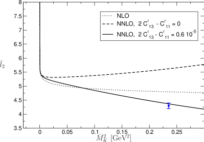
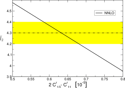
Figure 1: Left panel: Strange quark mass dependence of $\bar{l}_{2}$. As mentioned in the text, $\bar{M}_{K}$ denotes the kaon mass at one–loop accuracy in the limit $m_{u}=m_{d}=0$. The physical value of $m_{s}$ corresponds to $\bar{M}_{K}\approx 485$ MeV. We show the nlo (dotted line) as well as the nnlo result with two choices for $C^{\mathrm{r}}_{11,13}$: The dashed line corresponds to $2C^{\mathrm{r}}_{13}-C^{\mathrm{r}}_{11}=0$, while the solid line is evaluated at $2C^{\mathrm{r}}_{13}-C^{\mathrm{r}}_{11}=0.6\times 10^{-5}$, which reproduces the prediction from the dispersive analysis (data point with small error bar). Right panel: Dependence of $\bar{l}_{2}$ on the $p^{6}$ lecs $2C^{\mathrm{r}}_{13}-C^{\mathrm{r}}_{11}$ at the physical value of $m_{s}$. The dashed–dotted line with the error band corresponds to the data point and its error bar in the left panel. The running scale is taken at $\mu=M_{\rho}=770$ MeV, and $F_{0}=F_{\pi}=92.4$ MeV.

and illustrate the strange quark mass dependence of $\bar{l}_{2}$ in Fig.1 (left panel), where $\bar{l}_{2}$ is shown as a function of $\bar{M}_{K}^{2}$, at $\mu=M_{\rho}=770\mathrm{\,MeV},F_{0}=F_{\pi}=92.4\mathrm{\,MeV}$. The dotted line stands for the nlo approximation, and the nnlo result is shown for two choices for $C^{\mathrm{r}}_{11,13}$: the dashed (solid) line displays the case $2C^{\mathrm{r}}_{13}-C^{\mathrm{r}}_{11}=0$ ($2C^{\mathrm{r}}_{13}-C^{\mathrm{r}}_{11}=0.6\cdot 10^{-5}$). The solid line is constructed such that at the physical value of the strange quark mass, the lec $\bar{l}_{2}$ agrees with the measured one [17] , within the uncertainties.

We shortly comment on the $C^{\mathrm{r}}_{11,13}$ that occur in this application. In Ref. [19], $C^{\mathrm{r}}_{13}$ is worked out from an analysis of scalar form factors. While the result is of the order $2C^{\mathrm{r}}_{13}-C^{\mathrm{r}}_{11}=0.6\cdot 10^{-5}$, its precise value depends considerably on the input used, see table 2 in Ref. [19] for more information. In Ref. [20, table 12 (published version)] estimates for both lecs $C^{\mathrm{r}}_{11,13}$ are provided: the authors find that these do not receive a contribution from resonance exchange at leading order in large $N_{C}$ and therefore vanish at this order of accuracy. Because the scale at which this happens is not fixed a priori, that observation is not necessarily in contradiction with the above result.

The impact of these lecs on $\bar{l}_{2}$ is rather enhanced at physical strange quark masses. This is illustrated in Fig.1 (right panel). Taking the lecs $L_{j}^{\mathrm{r}}$ at face value, the window for a possible choice of the $C^{\mathrm{r}}_{11,13}$ is then very narrow to be in agreement with the data from a dispersive analysis. To pin down the $C^{\mathrm{r}}_{11,13}$ to good precision including an error analysis requires, however, a more thorough exploration. In particular, one has to take into account that in the fits performed in Ref. [18], an estimate of order $p^{6}$ counterterm contributions was already used.

5 LECs at order $\mathbf{p^{6}}$

The evaluation of all matching relations at two–loop order for the lecs at order $p^{6}$ is very complicated. To ease the calculations, we did not deal with the full framework in Ref. [2], but rather switched off the sources $s$ and $p$ (while retaining $m_{s}$). This yields the following simplifications:

1. the solution of the classical eom for the eta–field is trivial, $\eta=0$;

2. there is no mixing between the $\eta$ and the $\pi^{0}$ fields.

Point i) greatly simplifies the transition from the $\chi\text{\sc pt\rm}_{3}$ building blocks of the monomials to those of two flavours, as it suppresses any effects from the eta, whereas point ii) eliminates many possible graphs and hence considerably reduces the requested labour. For example, in this restricted framework, the one–particle reducible graphs (two one–loop diagrams linked by a single propagator) do not contribute to the matching, see Ref. [2].

Aiming for the $\mathcal{L}_{6}$-monomials in the generating functional requires the evaluation of many graphs with sunset–like topology. In the two–flavour limit, where one is interested in the local contributions only, one can simplify the loop calculations by using a short distance expansion for the massive propagators. This simplifies drastically the involved loop integrals; however, the contributions from individual graphs are not chirally invariant. Collecting terms stemming from different graphs to obtain a manifestly chirally invariant result is rather cumbersome. Since we are interested in the local terms only, we use a shortcut which is based on gauge invariance: one may choose a gauge such that at some fixed space–time point $x_{0}$, the totally symmetric combination of up to three derivatives acting on the chiral connection vanish,

$$\Gamma_{\mu}(x_{0})=0\;,\partial_{\{\mu}\Gamma_{\nu\}}(x_{0})=0\;,\partial_{\{\mu}\partial_{\nu}\Gamma_{\rho\}}(x_{0})=0\;,\partial_{\{\mu}\partial_{\nu}\partial_{\rho}\Gamma_{\sigma\}}(x_{0})=0\;.$$ (15)

Up to four ordinary derivatives are then indistinguishable from the fully symmetric combinations of covariant derivatives:

$$\partial_{\mu}f(x_{0})=\nabla_{\mu}f(x_{0})\;,\partial_{\mu}\partial_{\nu}f(x_{0})=\tfrac{1}{2}\{\partial_{\mu},\partial_{\nu}\}f(x_{0})=\tfrac{1}{2}\{\nabla_{\mu},\nabla_{\nu}\}f(x_{0})\;,\text{etc.}$$ (16)

This allows us to write even intermediate results in a manifestly chiral invariant manner.

To check our calculations in one corner, we matched the available $\chi\text{\sc pt\rm}_{2}$– and $\chi\text{\sc pt\rm}_{3}$–results for the vector–vector correlator [21] and for the pion form factor, worked out in Refs. [22, 23]. In this manner, we found that our relations for $c^{\mathrm{r}}_{56}$ and $c^{\mathrm{r}}_{51}-c^{\mathrm{r}}_{53}$ agree with the results of Refs. [22, 23]. Needless to say that this is quite a non–trivial check.

As already stated in Ref. [16], the monomial $P_{27}$ can be discarded from the $p^{6}$–Lagrangian for $\chi\text{\sc pt\rm}_{2}$. Therefore, the matching relations will certainly be a combination of some $c^{\mathrm{r}}_{i}$ and $c^{\mathrm{r}}_{27}$. Due to the restricted framework, only relations for lecs not involving monomials dependent on the sources $s$ or $p$ are nontrivial. In the restricted framework, there is an additional relation among the remaining $\mathrm{SU}(2)$–monomials:

$$\begin{split}&\tfrac{4}{3}P_{1}-\tfrac{1}{3}P_{2}+P_{3}-\tfrac{10}{3}P_{24}+\tfrac{4}{3}P_{25}+2P_{26}-\tfrac{8}{3}P_{28}-\tfrac{1}{2}P_{29}+\tfrac{1}{2}P_{30}-P_{31}+2P_{32}-\tfrac{1}{2}P_{33}\\ &+\tfrac{4}{3}P_{36}-\tfrac{4}{3}P_{37}-\tfrac{11}{6}P_{39}+\tfrac{5}{6}P_{40}+\tfrac{7}{3}P_{41}-\tfrac{4}{3}P_{42}-\tfrac{3}{2}P_{43}+\tfrac{1}{2}P_{44}-\tfrac{1}{2}P_{45}-P_{51}-P_{53}=0\;.\end{split}$$ (17)

Because the eom is different in the full framework, this relation is no longer valid there. We used Eq. (17) to exclude the monomial $P_{1}$ from our consideration. As a result, we give the matching for the 27 combinations of $c^{\mathrm{r}}_{i}$ displayed in table 1. In the full framework, an additional matching relation (apart from the ones for the monomials involving the sources $s$ and $p$) for $c^{\mathrm{r}}_{1}$ could be worked out, yielding the only missing piece in the matching for the 28 lecs worked out here.

The final result may be written in the form

$$x_{i}=p^{(0)}_{i}+p^{(1)}_{i}\ell_{K}+p^{(2)}_{i}\ell_{K}^{2}+O(m_{s})\;,$$ (18)

where $x_{i}$ denotes one of the 27 linear combinations of the $c^{\mathrm{r}}_{i}$ displayed in table 1. The explicit expressions for the polynomials $p^{(n)}_{i}$ in the $\chi\text{\sc pt\rm}_{3}$–lecs are displayed in tables 2 and 3 of our article [2].

$i$	$x_{i}$	$i$	$x_{i}$	$i$	$x_{i}$
1	$c^{\mathrm{r}}_{2}+\frac{1}{4}c^{\mathrm{r}}_{1}$	10	$c^{\mathrm{r}}_{32}-\frac{3}{2}c^{\mathrm{r}}_{1}-c^{\mathrm{r}}_{27}$	19	$c^{\mathrm{r}}_{43}+\frac{9}{8}c^{\mathrm{r}}_{1}+\frac{1}{4}c^{\mathrm{r}}_{27}$
2	$c^{\mathrm{r}}_{3}-\frac{3}{4}c^{\mathrm{r}}_{1}$	11	$c^{\mathrm{r}}_{33}+\frac{3}{8}c^{\mathrm{r}}_{1}+\frac{1}{4}c^{\mathrm{r}}_{27}$	20	$c^{\mathrm{r}}_{44}-\frac{3}{8}c^{\mathrm{r}}_{1}-\frac{1}{4}c^{\mathrm{r}}_{27}$
3	$c^{\mathrm{r}}_{24}+\frac{5}{2}c^{\mathrm{r}}_{1}$	12	$c^{\mathrm{r}}_{36}-c^{\mathrm{r}}_{1}$	21	$c^{\mathrm{r}}_{45}+\frac{3}{8}c^{\mathrm{r}}_{1}+\frac{1}{4}c^{\mathrm{r}}_{27}$
4	$c^{\mathrm{r}}_{25}-c^{\mathrm{r}}_{1}$	13	$c^{\mathrm{r}}_{37}+c^{\mathrm{r}}_{1}$	22	$c^{\mathrm{r}}_{50}$
5	$c^{\mathrm{r}}_{26}-\frac{3}{2}c^{\mathrm{r}}_{1}$	14	$c^{\mathrm{r}}_{38}$	23	$c^{\mathrm{r}}_{51}+\frac{3}{4}c^{\mathrm{r}}_{1}+\frac{1}{2}c^{\mathrm{r}}_{27}$
6	$c^{\mathrm{r}}_{28}+2c^{\mathrm{r}}_{1}-c^{\mathrm{r}}_{27}$	15	$c^{\mathrm{r}}_{39}+\frac{11}{8}c^{\mathrm{r}}_{1}+\frac{1}{4}c^{\mathrm{r}}_{27}$	24	$c^{\mathrm{r}}_{52}$
7	$c^{\mathrm{r}}_{29}+\frac{3}{8}c^{\mathrm{r}}_{1}+\frac{1}{4}c^{\mathrm{r}}_{27}$	16	$c^{\mathrm{r}}_{40}-\frac{5}{8}c^{\mathrm{r}}_{1}-\frac{1}{4}c^{\mathrm{r}}_{27}$	25	$c^{\mathrm{r}}_{53}+\frac{3}{4}c^{\mathrm{r}}_{1}+\frac{1}{2}c^{\mathrm{r}}_{27}$
8	$c^{\mathrm{r}}_{30}-\frac{3}{8}c^{\mathrm{r}}_{1}-\frac{1}{4}c^{\mathrm{r}}_{27}$	17	$c^{\mathrm{r}}_{41}-\frac{7}{4}c^{\mathrm{r}}_{1}-\frac{1}{2}c^{\mathrm{r}}_{27}$	26	$c^{\mathrm{r}}_{55}$
9	$c^{\mathrm{r}}_{31}+\frac{3}{4}c^{\mathrm{r}}_{1}+\frac{1}{2}c^{\mathrm{r}}_{27}$	18	$c^{\mathrm{r}}_{42}+c^{\mathrm{r}}_{1}$	27	$c^{\mathrm{r}}_{56}$

Table 1: The quantities $x_{i}$ in Eq. (18)

6 Summary

In this talk, we have discussed a general procedure [1, 2] to work out the matching relations between the lecs in $\chi\text{\sc pt\rm}_{2}$ and $\chi\text{\sc pt\rm}_{3}$ in a perturbative manner. For the lecs at order $p^{2}$ and $p^{4}$, and for a subset of those at order $p^{6}$, the relations are now available at two–loop order. The method could be used with only moderate adaption to work out more general matching relations, like the ones for $\chi\text{\sc pt\rm}_{N-1}$ to $\chi\text{\sc pt\rm}_{N}$. To obtain the matching relations of the the remaining lecs at order $p^{6}$ to the same accuracy would require, however, a very big amount of work.

We have in addition illustrated the use of the results in the case of $l_{2}^{\mathrm{r}}$: its precise knowledge, together with the known values of $L_{2}^{\mathrm{r}},L_{3}$, in principle allows one to pin down the combination $2C^{\mathrm{r}}_{13}-C^{\mathrm{r}}_{11}$ rather precisely.

We refer the interested reader to our articles Refs. [1, 2] for the matching relations found, and for further details on the method used.

References

• [1] J. Gasser, C. Haefeli, M. A. Ivanov and M. Schmid, Phys. Lett.  B 652 (2007) 21
[arXiv:0706.0955 [hep-ph]].
• [2] J. Gasser, C. Haefeli, M. A. Ivanov and M. Schmid, Phys. Lett.  B 675 (2009) 49
[arXiv:0903.0801 [hep-ph]].
• [3] S. Weinberg, Physica A 96 (1979) 327.
• [4] J. Gasser and H. Leutwyler, Annals Phys.  158 (1984) 142.
• [5] J. Gasser and H. Leutwyler, Nucl. Phys.  B 250 (1985) 465.
• [6] R. Kaiser and J. Schweizer, JHEP 0606 (2006) 009 [arXiv:hep-ph/0603153].
• [7] B. Moussallam, JHEP 0008 (2000) 005 [arXiv:hep-ph/0005245].
• [8] K. Kampf and B. Moussallam, Phys. Rev.  D 79 (2009) 076005 [arXiv:0901.4688 [hep-ph]].
• [9] M. Frink and U. G. Meissner, JHEP 0407 (2004) 028 [arXiv:hep-lat/0404018].
• [10] M. Mai, P. C. Bruns, B. Kubis and U. G. Meissner, Phys. Rev.  D 80 (2009) 094006
[arXiv:0905.2810 [hep-ph]].
• [11] J. Gasser, V. E. Lyubovitskij, A. Rusetsky and A. Gall, Phys. Rev.  D 64 (2001) 016008 [arXiv:hep-ph/0103157].
• [12] H. Jallouli and H. Sazdjian, Phys. Rev.  D 58 (1998) 014011 [Erratum-ibid.  D 58 (1998) 099901] [arXiv:hep-ph/9706450].
• [13] A. Nehme, La Brisure d’Isospin dans les Interactions Meson–Meson à Basse Energie, PhD thesis, CPT Marseille, July 2002.
• [14] C. Haefeli, M. A. Ivanov and M. Schmid, Eur. Phys. J.  C 53 (2008) 549 [arXiv:0710.5432 [hep-ph]].
• [15] J. Bijnens, G. Colangelo and G. Ecker, JHEP 9902 (1999) 020 [hep-ph/9902437].
• [16] C. Haefeli, M. A. Ivanov, M. Schmid and G. Ecker, arXiv:0705.0576 [hep-ph].
• [17] G. Colangelo, J. Gasser and H. Leutwyler, Nucl. Phys.  B 603 (2001) 125 [hep-ph/0103088].
• [18] G. Amoros, J. Bijnens and P. Talavera, Nucl. Phys.  B 602 (2001) 87 [hep-ph/0101127].
• [19] J. Bijnens and P. Dhonte, JHEP 0310 (2003) 061 [hep-ph/0307044].
• [20] V. Cirigliano et al., Nucl. Phys.  B 753 (2006) 139 [hep-ph/0603205].
• [21] G. Amoros, J. Bijnens and P. Talavera, Nucl. Phys.  B 568 (2000) 319 [arXiv:hep-ph/9907264].
• [22] J. Bijnens, G. Colangelo and P. Talavera, JHEP 9805 (1998) 014 [arXiv:hep-ph/9805389].
• [23] J. Bijnens and P. Talavera, JHEP 0203 (2002) 046 [arXiv:hep-ph/0203049].