.

Abstract. The standard covariant differentiation procedure for fields in vector bundles is generalised so as to be applicable to fields in general nonaffine bundles in which the fibres may have an arbitrary nonlinear structure. In addition to the usual requirement that the base space should be flat or endowed with its own linear connection ${\color[rgb]{0,0,.66}\Gamma}$, and that there should be an ordinary gauge connection ${\color[rgb]{.66,0,.33}\bf{A}}$ on the bundle, it is necessary to require also that there should be an intrinsic, bundle-group invariant connection $\hat{\color[rgb]{1,0,0}{\Gamma}}$ on the fibre space. The procedure is based on the use of an appropriate primary-field (i.e. section) independent connector ${\color[rgb]{.66,0,.33}\omega}$ that is constructed in terms of the natural fibre-tangent-vector realisation of the gauge connection ${\color[rgb]{.66,0,.33}\bf{A}}$. The application to gauged harmonic mappings will be described in a following article.

1 Introduction

Since at least the time of Clerk-Maxwell, or even earlier, nearly all the most successsful physical models for the description of the physical world at a fundamental (and also often at a higher) level have been essentially based on the conceptual framework of local field theory. The fields in question, whose behaviour is governed by local differential equations of usually not higher than second order, are generally interpretable – at a classical level – as sections of fibre bundles over some appropriate base space (which might, for example represent ordinary four-dimensional space-time, or some higher-dimensional extension or lower-dimensional subspace therof).

In the most familiar and well developed examples (including Yang-Mills theory), although the theories themselves may be nonlinear (in the sense that the field equations contain coupling terms of quadratic or higher order) the actual fields are intrinsically linear in so much as they belong to bundles whose fibres are flat. In the simplest cases the fibre space is actually vectorial, and even in the case of gauge-connection fields (e.g. of Yang-Mills type) the fibre space still has a well defined affine structure, although there is no longer any preferred origin. For fields in such essentially linear (i.e. affinely fibreed) bundles, the standard procedure for the construction of the relevant gauge-covariant derivatives (in terms of which the field equations are expressed) provided an appropriate connection is available, is widely known and familiar (see e.g. Choquet Bruhat, Morette-DeWitt, Bleck-Dillard [1]).

The main purpose of the present work is to describe how the standard machinery for gauge covariant differentiation can be generalised so as to be applicable to fields that are intrinsically nonlinear, in the sense of being sections of nonaffinely fibered bubdles. Such nonaffine fields (as exemplified by nonlinear $\sigma$ models) have attracted an increasing amount of interest in recent years.

The usual procedure for ordinary vector bundles needs the provision only of a gauge connection ${\color[rgb]{.66,0,.33}\bf{A}}$, in addition to thee requirement that the base space should either be flat or at least provided with an ordinary linear connection ${\color[rgb]{0,0,.66}\Gamma}$. The natural generalization to be described here requires also that the (curved) fibre space should be provided with its own linear connection $\hat{\color[rgb]{1,0,0}{\Gamma}}$.

In a following article we shall describe the application of the general purpose formalism set up below to the particular case of a Riemannian connection induced automatically by the Lagrangian for the natural minimally gauge coupled generalisation of the class of harmonic mappings that was described by Misner [2]. These gauged-harmonic mappings will include as a special case the gauge-coupled generalization of the nonlinear $\sigma$ model with fully homogeneous symmetric fibres that was recently described by the present author [3].

2 The concepts of bitensorial differentiation and connector fields

One of the essential guidelines whose observance qualifies a theoretical treatment for description as geometric is the requirement that one should work as far as possible in terms of entities that are invariant in the sense of being independent of any arbitrarily chosen system of reference that one might wish to introduce for the sake of explicitness at some inremediate stage in the treatment. However, the strictest observance of this precept risks giving a treatment that either needs to be unduly abstract as the price of being elegant or else that needs unweildy mathematical machinery as the price of being concrete. For this reason most theoretical physicists do not insist on the exclusive use of entities that are strictly invariant, but as a compromise prefer nevertheless to work as far as possible with entities that are at least covariant in the sense of being subject to simply described rules of variation when the relevant reference system is altered. One of the simplest and most convenient examples is that of quantities represented in terms of sets of components whose rules of variation are of tensorial type in the sense of being expressible in terms of appropriate contractions with relevant coordinate transformation matrices. In the specific context of general field theories we shall be particularly concerned with entities whose covariance is of bitensorial in so much as they involve two independent matrices expressing independent coordinate changes on the base and fibre spaces respectively.

As a basic starting point let us consider the case of field ${\color[rgb]{1,0,0}{V}}$ of simple vectorial type, meaning that its components ${\color[rgb]{1,0,0}{V}}^{{}_{\color[rgb]{1,0,0}{A}}}$ undergo a change of the form

$${\color[rgb]{1,0,0}{V}}^{{}_{\color[rgb]{1,0,0}{A}}}\ \mapsto\ {\color[rgb]{.66,0,.33}{G}}^{{}_{\color[rgb]{1,0,0}{A}}}_{\ {}_{\color[rgb]{1,0,0}{B}}}{\color[rgb]{1,0,0}{V}}^{{}_{\color[rgb]{1,0,0}{B}}}$$ (1)

under the effect of a fibre-coordinate transformation characterised by the matrix $G^{{}_{\color[rgb]{1,0,0}{A}}}_{\ {}_{\color[rgb]{1,0,0}{B}}}$. Suppose that we simultaneously carry out a coordinate transformation

$$x^{\mu}\mapsto y^{\mu}\{x\}$$ (2)

on the base space ${\cal M}$ over which the field ${\color[rgb]{1,0,0}{V}}$ is defined, thereby determining a corresponding base-space transformation matrix given by

$$Q^{\mu}_{\ \nu}=\partial_{\nu}y^{\mu}\,,$$ (3)

where we have introduced the abbreviation

$$\partial_{\mu}=\frac{\partial}{\partial x^{\mu}}$$

for partial coordinate differentiation of a field over the base space. Then the components

$${\color[rgb]{.66,0,.33}{D}}_{\mu}{\color[rgb]{1,0,0}{V}}^{{}_{\color[rgb]{1,0,0}{A}}}=\partial_{\mu}{\color[rgb]{1,0,0}{V}}^{{}_{\color[rgb]{1,0,0}{A}}}+{\color[rgb]{.66,0,.33}\omega}_{\mu\ _{\color[rgb]{1,0,0}{B}}}^{\ {}_{\color[rgb]{1,0,0}{A}}}{\color[rgb]{1,0,0}{V}}^{{}_{\color[rgb]{1,0,0}{B}}}$$ (4)

will qualify for description as those of a covariant or more explicitly bitensorial derivative if they transform according to the corresponding matrix contraction rule as expressed by

$${\color[rgb]{.66,0,.33}{D}}_{\mu}{\color[rgb]{1,0,0}{V}}^{{}_{\color[rgb]{1,0,0}{A}}}\mapsto Q^{-1\nu}_{\,\ \ \ \mu}{\color[rgb]{.66,0,.33}{G}}^{{}_{\color[rgb]{1,0,0}{A}}}_{\ {}_{\color[rgb]{1,0,0}{B}}}\,{\color[rgb]{.66,0,.33}{D}}_{\nu}{\color[rgb]{1,0,0}{V}}^{{}_{\color[rgb]{1,0,0}{B}}}\,.$$ (5)

It is evident that the bitensorial covariance property (5) will hold if and only if the components ${\color[rgb]{.66,0,.33}\omega}_{\mu\ _{\color[rgb]{1,0,0}{B}}}^{\ {}_{\color[rgb]{1,0,0}{A}}}$ have a covariance property of a rather more complicated nature, namely

$${\color[rgb]{.66,0,.33}\omega}_{\mu\ _{\color[rgb]{1,0,0}{B}}}^{\ {}_{\color[rgb]{1,0,0}{A}}}\ \mapsto\ Q^{-1\nu}_{\,\ \ \ \mu}{\color[rgb]{.66,0,.33}{G}}^{-1_{\color[rgb]{1,0,0}{C}}}_{\,\ \ \ {}_{\color[rgb]{1,0,0}{B}}}({\color[rgb]{.66,0,.33}{G}}^{{}_{\color[rgb]{1,0,0}{A}}}_{\ {}_{\color[rgb]{1,0,0}{D}}}{\color[rgb]{.66,0,.33}\omega}_{\nu\ _{\color[rgb]{1,0,0}{D}}}^{\ {}_{\color[rgb]{1,0,0}{C}}}-\partial_{\nu}{\color[rgb]{.66,0,.33}{G}}^{{}_{\color[rgb]{1,0,0}{A}}}_{\ {}_{\color[rgb]{1,0,0}{C}}})\,.$$ (6)

This will be of bitensorial form only if the base gradient $\partial_{\mu}{\color[rgb]{.66,0,.33}{G}}^{{}_{\color[rgb]{1,0,0}{A}}}_{\ {}_{\color[rgb]{1,0,0}{B}}}$ of the the fibre-coordinate transformation matrix ${\color[rgb]{.66,0,.33}{G}}^{{}_{\color[rgb]{1,0,0}{A}}}_{\ {}_{\color[rgb]{1,0,0}{B}}}$ happens to vanish (which will not in general be the case for the examples we wish to consider).

We shall use the term connector to denote any field ${\color[rgb]{.66,0,.33}\omega}$ having components ${\color[rgb]{.66,0,.33}\omega}_{\mu\ _{\color[rgb]{1,0,0}{B}}}^{\ {}_{\color[rgb]{1,0,0}{A}}}$ specified by one (covariant) base-coordinate index and two (mixed) fibre-coordinate indices and transforming according to the rule (6). A connector can be considered as a special kind of biaffinator, using the term affinator as an abbreviation for affine tensor, to denote quantities whose components transform according to a rule that generalises the ordinary kind of tensorial transformation law by allowing for the presence of an inhomogeneous additive term [having the form $-Q^{-1\nu}_{\,\ \ \ \mu}{\color[rgb]{.66,0,.33}{G}}^{-1_{\color[rgb]{1,0,0}{C}}}_{\,\ \ \ {}_{\color[rgb]{1,0,0}{B}}}\,\partial_{\nu}{\color[rgb]{.66,0,.33}{G}}^{{}_{\color[rgb]{1,0,0}{A}}}_{\ {}_{\color[rgb]{1,0,0}{C}}}$ in the example (6)] over and above the usual homogeneous multiplicative term [having the form $Q^{-1\nu}_{\,\ \ \ \mu}{\color[rgb]{.66,0,.33}{G}}^{-1_{\color[rgb]{1,0,0}{C}}}_{\,\ \ \ {}_{\color[rgb]{1,0,0}{B}}}{\color[rgb]{.66,0,.33}{G}}^{{}_{\color[rgb]{1,0,0}{A}}}_{\ {}_{\color[rgb]{1,0,0}{D}}}{\color[rgb]{.66,0,.33}\omega}_{\nu\ _{\color[rgb]{1,0,0}{D}}}^{\ {}_{\color[rgb]{1,0,0}{C}}}$ in the example (6)].

Insomuch as it is subject to the bi-aftensorial transformation (6), a connector ${\color[rgb]{.66,0,.33}\omega}$ can be interpreted as a genuine field in the sense that it is a section in an appropriately constructed fibre bundle ${\color[rgb]{.66,0,.33}{\cal C}}^{\prime}$ over the base space ${\cal M}$, the bundle being of affine (rather than ordinary vectorial) kind in the sense that (as well as being subject to the usual group of homogeneous base-coordinate transformations specified by the matrices $Q^{\nu}_{\ \mu}$) the fibres of the bundle are subject to an action of the associated inhomogeneous adjoint group ${\color[rgb]{.66,0,.33}{\cal G}}^{\prime\dagger}$ of linear transformations generated by uniform translations and by the adjoint action of the matrices ${\color[rgb]{.66,0,.33}{G}}^{{}_{\color[rgb]{1,0,0}{A}}}_{\ {}_{\color[rgb]{1,0,0}{B}}}$.

We use the term connector (as distinct from connection) for the purpose of emphasizing this interpretation of ${\color[rgb]{.66,0,.33}\omega}$ as a genuine (biaffinitorial) field in the sense of being a section in the relevant (affine) fibre bundle ${\color[rgb]{.66,0,.33}{\cal C}}^{\prime}$, as chararacterized by an action of the corresponding inhomogeneous adjoint group ${\color[rgb]{.66,0,.33}{\cal G}}^{\prime\dagger}$. Of course, such an ${\color[rgb]{.66,0,.33}\omega}$ can also be given a more traditional mathematical interpretation as a connection, meaning an algebra-valued form on an appropriate principal fibre bundle ${\color[rgb]{.66,0,.33}{\cal P}}^{\prime}$ (see e.g. Choque-Bruhat et al.[1] or Carter [4]) associated with the corresponding vector bundle ${\color[rgb]{1,0,0}{\cal V}}^{\prime}$ containing ${\color[rgb]{1,0,0}{V}}$, as characterised by the left action on itself of the subgroup ${\color[rgb]{.66,0,.33}{\cal G}}^{\prime}$ of ${\color[rgb]{.66,0,.33}{\cal G}}^{\prime\dagger}$ generated directly by the multiplicative action of the allowed transformation matrices ${\color[rgb]{.66,0,.33}{G}}^{{}_{\color[rgb]{1,0,0}{A}}}_{\ {}_{\color[rgb]{1,0,0}{B}}}$.

The need for rather more care that usual in the interpretation of ${\color[rgb]{.66,0,.33}\omega}$ – either as a connector in $\,{\color[rgb]{.66,0,.33}{\cal C}}^{\prime}$ or as a connection on $\,{\color[rgb]{.66,0,.33}{\cal P}}^{\prime}$ – arises in situations where our primary purpose is to deal with differentiation of a primary field ${\color[rgb]{1,0,0}{\Phi}}$ having values in a nonaffinely fibered bundle ${\color[rgb]{1,0,0}{\cal B}}$ subject to the provision of an ordinary gauge field ${\color[rgb]{.66,0,.33}\bf{A}}$ with respect to the bundle group ${\color[rgb]{.66,0,.33}{\cal G}}$ of ${\color[rgb]{1,0,0}{\cal B}}$. Such a gauge field ${\color[rgb]{.66,0,.33}\bf{A}}$ will be interpretable in the traditional way as a connection on the directly associated principle bundle ${\color[rgb]{.66,0,.33}{\cal P}}$ of ${\color[rgb]{1,0,0}{\cal B}}$ (with nonlinear fibres having the form of ${\color[rgb]{.66,0,.33}{\cal G}}$ itself) and it will also be interpretable as a connector field in an appropriate affine bundle ${\color[rgb]{.66,0,.33}{\cal C}}$ subject to the action of the inhomogeneous adjoint group ${\color[rgb]{.66,0,.33}{\cal G}}^{\dagger}$ associated with ${\color[rgb]{.66,0,.33}{\cal G}}$ (as well as base coordinate transformations) on the fibres.

This primary connector bundle ${\color[rgb]{.66,0,.33}{\cal C}}$, containing the gauge section ${\color[rgb]{.66,0,.33}\bf{A}}$ will in the general case (for a nonlinearly fibered primary bundle ${\color[rgb]{1,0,0}{\cal B}}$) be distinct from what we shall refer to as the derived principle bundle ${\color[rgb]{.66,0,.33}{\cal P}}^{\prime}$ and the derived connector ${\color[rgb]{.66,0,.33}\omega}$ (for which the corresponding groups ${\color[rgb]{.66,0,.33}{\cal G}}^{\prime}$ and ${\color[rgb]{.66,0,.33}{\cal G}}^{\prime\dagger}$ may be larger than ${\color[rgb]{.66,0,.33}{\cal G}}$ and ${\color[rgb]{.66,0,.33}{\cal G}}^{\dagger}$). These derived bundles and the connector ${\color[rgb]{.66,0,.33}\omega}$ are not (in the nonlinear case) determined in advance by the corresponding primary bundles and the gauge field ${\color[rgb]{.66,0,.33}\bf{A}}$, but are specified as functions of the section ${\color[rgb]{1,0,0}{\Phi}}$ in ${\color[rgb]{1,0,0}{\cal B}}$. Any such section immediately determines a corresponding bundle ${\color[rgb]{1,0,0}{\cal V}}^{\prime}$ of ordinary vectorial type (over the same base ${\cal M}$ whose elements ${\color[rgb]{1,0,0}{V}}$ are just the tangent vectors to the fibres of ${\color[rgb]{1,0,0}{\cal B}}$ at the section ${\color[rgb]{1,0,0}{\Phi}}$. This section dependent vector bundle ${\color[rgb]{1,0,0}{\cal V}}^{\prime}$ is the basic building block from which, in conjunction with the ordinary cotangeent bundle over ${\cal M}$, one can proceed to construct the corresponding tensorially associated vector bundles that are needed to contain bitensorial derivatives of various orders. The derived bundles ${\color[rgb]{.66,0,.33}{\cal P}}^{\prime}$ or ${\color[rgb]{.66,0,.33}{\cal C}}^{\prime}$ that are needed for the definition – as, respectively, a connection or a section – of the connector ${\color[rgb]{.66,0,.33}\omega}$ that will be required (for the explicit construction of such bitensorial covariant derivatives) will be, respectively, the directly associated principle bundle ${\color[rgb]{.66,0,.33}{\cal P}}^{\prime}$ of ${\color[rgb]{1,0,0}{\cal V}}^{\prime}$ or the corresponding affine bundle ${\color[rgb]{.66,0,.33}{\cal C}}^{\prime}$ as characterized by the bundle group ${\color[rgb]{.66,0,.33}{\cal G}}^{\prime}$ of ${\color[rgb]{1,0,0}{\cal V}}^{\prime}$ and of its (inhomogeneous adjoint) extension ${\color[rgb]{.66,0,.33}{\cal G}}^{\prime\dagger}$ acting on ${\color[rgb]{.66,0,.33}{\cal C}}^{\prime}$.

The possibility that the derived bundle group ${\color[rgb]{.66,0,.33}{\cal G}}^{\prime}$ may be considerably larger than the primary bundle group ${\color[rgb]{.66,0,.33}{\cal G}}$ results from the fact that it arises from (in general, base -position dependent) fibre coordinate transformations

$${\color[rgb]{1,0,0}{X}}^{{}_{\color[rgb]{1,0,0}{A}}}\{{\color[rgb]{1,0,0}{X}},x\}\ \mapsto\ {\color[rgb]{.66,0,.33}{G}}^{{}_{\color[rgb]{1,0,0}{A}}}\{{\color[rgb]{1,0,0}{X}},x\}$$ (7)

for ${\color[rgb]{1,0,0}{X}}\in{\color[rgb]{1,0,0}{\cal X}}$, $x\in{\cal M}$, where ${\cal M}$ is the base space and ${\color[rgb]{1,0,0}{\cal X}}$ the fibre space of ${\color[rgb]{1,0,0}{\cal B}}$, that arise not only from the action of the primary gauge group ${\color[rgb]{.66,0,.33}{\cal G}}$ but also from the group of non linear transformations between coordinates of the different patches that may be needed to cover the fibre space ${\color[rgb]{1,0,0}{\cal X}}$ when it has itself a nonlinear manifold structure. In terms of the original fibre coordinates ${\color[rgb]{1,0,0}{X}}^{{}_{\color[rgb]{1,0,0}{A}}}$, the elements of ${\color[rgb]{.66,0,.33}{\cal G}}^{\prime}$ will be represented by matrices of the form

$${\color[rgb]{.66,0,.33}{G}}^{{}_{\color[rgb]{1,0,0}{A}}}_{\ {}_{\color[rgb]{1,0,0}{B}}}\{{\color[rgb]{1,0,0}{X}},x\}={\color[rgb]{.66,0,.33}{G}}^{{}_{\color[rgb]{1,0,0}{A}}}_{\ ,_{\color[rgb]{1,0,0}{B}}}$$ (8)

as evaluated on the chosed section

$${\color[rgb]{1,0,0}{X}}={\color[rgb]{1,0,0}{\Phi}}\{x\}\,,$$ (9)

where a comma denotes partial differentiation, so that, in particular, the total space gradient components (with respect to the local coordinates $x^{\mu}$ and ${\color[rgb]{1,0,0}{X}}^{{}_{\color[rgb]{1,0,0}{A}}}$) that appear in the connector transformation formula (6) will be given explicitly by

$$\partial_{\mu}{\color[rgb]{.66,0,.33}{G}}^{{}_{\color[rgb]{1,0,0}{A}}}_{\ {}_{\color[rgb]{1,0,0}{B}}}={\color[rgb]{.66,0,.33}{G}}^{{}_{\color[rgb]{1,0,0}{A}}}_{\ ,_{\color[rgb]{1,0,0}{B}},\mu}+{\color[rgb]{.66,0,.33}{G}}^{{}_{\color[rgb]{1,0,0}{A}}}_{\ ,_{\color[rgb]{1,0,0}{B}},_{\color[rgb]{1,0,0}{C}}}{\color[rgb]{1,0,0}{\Phi}}^{{}_{\color[rgb]{1,0,0}{C}}}_{\ ,\mu}\ ,$$ (10)

where

$${\color[rgb]{1,0,0}{\Phi}}^{{}_{\color[rgb]{1,0,0}{C}}}={\color[rgb]{1,0,0}{X}}^{{}_{\color[rgb]{1,0,0}{C}}}\{{\color[rgb]{1,0,0}{\Phi}}\{x\}\}\,.$$

In the following sections we shall describe the natural procedure for explicitly constructing a well defined section dependent connector field ${\color[rgb]{.66,0,.33}\omega}$ obeying the rule (7), in terms of a previously given primary gauge field ${\color[rgb]{.66,0,.33}\bf{A}}$ and of ordinary linear connections ${\color[rgb]{0,0,.66}\Gamma}$ and $\hat{\color[rgb]{1,0,0}{\Gamma}}$ on the base and fibre spaces ${\cal M}$ and ${\color[rgb]{1,0,0}{\cal X}}$ respectively. Before doing so we remark that because such a section-dependent connector can be interpreted as as an ordinary connection on the artificially constructed (section dependent) vector bundle ${\color[rgb]{1,0,0}{\cal V}}^{\prime}$, it follows that ${\color[rgb]{.66,0,.33}\omega}$ will automatically have the usual properties that are familiar from the standard theory of fixed (section-independent) connections. In particular, the connector ${\color[rgb]{.66,0,.33}\omega}$ will determine a corresponding well-defined (but section dependent) bitensorial curvature field ${\color[rgb]{.66,0,.33}\Omega}$ according to a formula of the familiar form

$${\color[rgb]{.66,0,.33}\Omega}_{\mu\nu\ _{\color[rgb]{1,0,0}{B}}}^{\,\ \ {}_{\color[rgb]{1,0,0}{A}}}=2\partial_{[\mu}\,{\color[rgb]{.66,0,.33}\omega}_{\nu]\ _{\color[rgb]{1,0,0}{B}}}^{\,\ {}_{\color[rgb]{1,0,0}{A}}}+2{\color[rgb]{.66,0,.33}\omega}_{[\mu\ |_{\color[rgb]{1,0,0}{C}}|}^{\,\ {}_{\color[rgb]{1,0,0}{A}}}{\color[rgb]{.66,0,.33}\omega}_{\nu]\ _{\color[rgb]{1,0,0}{B}}}^{\ {}_{\color[rgb]{1,0,0}{C}}}$$ (11)

(where square brackets denote antisymmetrisation) and this field will satisfy a Bianchi identity of the familiar form

$$\partial_{[\mu}{\color[rgb]{.66,0,.33}\Omega}_{\nu\rho]\ _{\color[rgb]{1,0,0}{B}}}^{\ \ \ {}_{\color[rgb]{1,0,0}{A}}}={\color[rgb]{.66,0,.33}\Omega}_{[\mu\nu\ |_{\color[rgb]{1,0,0}{C}}|}^{\ \ \ {}_{\color[rgb]{1,0,0}{A}}}{\color[rgb]{.66,0,.33}\omega}_{\rho]\ _{\color[rgb]{1,0,0}{B}}}^{\,\ {}_{\color[rgb]{1,0,0}{C}}}-{\color[rgb]{.66,0,.33}\omega}_{[\mu\ |_{\color[rgb]{1,0,0}{C}}|}^{\ \ {}_{\color[rgb]{1,0,0}{A}}}{\color[rgb]{.66,0,.33}\Omega}_{\nu\rho]\,\ _{\color[rgb]{1,0,0}{B}}}^{\ \ \ {}_{\color[rgb]{1,0,0}{C}}}\,.$$ (12)

3 Bitensorial differentiation in the absence of a gauge transformation

Before dealing with the general situation (where there is a non-trivial gauge group ${\color[rgb]{.66,0,.33}{\cal G}}$) let us start by dealing with the comparitively simple case for which the fundamental bundle ${\color[rgb]{1,0,0}{\cal B}}$ under consideration is endowed with a trivial direct product structure ${\color[rgb]{1,0,0}{\cal X}}\times{\cal M}$ where ${\cal M}$ is the base space, with local coordinates $x^{\mu}$, and ${\color[rgb]{1,0,0}{\cal X}}$ is the fibre space, with local coordinates ${\color[rgb]{1,0,0}{X}}^{{}_{\color[rgb]{1,0,0}{A}}}$. The imposition of such a diresct product structure is equivalent to the specification of an integrable connection on the bundle. Its presence enables us to restrict our attention for the time being to fibre-coordinate transformations

$${\color[rgb]{1,0,0}{X}}^{{}_{\color[rgb]{1,0,0}{A}}}\{{\color[rgb]{1,0,0}{X}}\}\ \mapsto\ {\color[rgb]{1,0,0}{Y}}^{{}_{\color[rgb]{1,0,0}{A}}}\{{\color[rgb]{1,0,0}{X}}\}$$ (13)

that are independent of base position, i.e. such that

$${\color[rgb]{1,0,0}{Y}}^{{}_{\color[rgb]{1,0,0}{A}}}_{\ ,\mu}=0\,,$$ (14)

unlike the more general transformations of the form (7) that were mentioned in the introduction and to which we shalll return in the next section.

In such integrable cases the procedure described by Misner[2] for the Riemannian case can be taken over directly provided that the base ${\cal M}$ and the fibre ${\color[rgb]{1,0,0}{\cal X}}$ each has its own linear connection. An ordinary linear connection on ${\cal M}$ will be specified by a corresponding purely affinitorial (as opposed to the more general biaffinitorial) connector field ${\color[rgb]{0,0,.66}\Gamma}$ with mixed components ${\color[rgb]{0,0,.66}\Gamma}_{\!\mu\ \rho}^{\ \nu}$ which can be used, e.g. for a simple tangent vector ${\color[rgb]{0,0,.66}v}$ with components ${\color[rgb]{0,0,.66}v}^{\mu}$, to specify the covariant variation $\hbox to0.0pt{\raise 4.0pt\hbox{\color[rgb]{0,0,.66}{\,\bf-}}\hss}{\rm d}{\color[rgb]{0,0,.66}v}$ with components $(\hbox to0.0pt{\raise 4.0pt\hbox{\color[rgb]{0,0,.66}{\,\bf-}}\hss}{\rm d}{\color[rgb]{0,0,.66}v})^{\mu}$ associated with an infinitesimal component variation ${\rm d}({\color[rgb]{0,0,.66}v}^{\mu})$ in conjunction with a base displacement ${\rm d}x^{\mu}$ by the formula

$$\hbox to0.0pt{\raise 4.0pt\hbox{\color[rgb]{0,0,.66}{\,\bf-}}\hss}{\rm d}{\color[rgb]{0,0,.66}v}^{\mu}={\rm d}({\color[rgb]{0,0,.66}v}^{\mu})+{\color[rgb]{0,0,.66}\Gamma}_{\!\nu\ \rho}^{\ \mu}\,{\color[rgb]{0,0,.66}v}^{\rho}\,{\rm d}x^{\nu}$$ (15)

so that if ${\color[rgb]{0,0,.66}v}$ is defined as a field over ${\cal M}$ there will be a corresponding tensorial covariant differentiation operator ${\color[rgb]{0,0,.66}\nabla}$ whose effect is given by

$${\color[rgb]{0,0,.66}\nabla}_{\!\nu}{\color[rgb]{0,0,.66}v}^{\mu}=\partial_{\mu}{\color[rgb]{0,0,.66}v}^{\mu}+{\color[rgb]{0,0,.66}\Gamma}_{\!\mu\ \rho}^{\ \nu}\,{\color[rgb]{0,0,.66}v}^{\rho}\,.$$ (16)

In an exactly analogous manner, the connection on the fibre space will be specified by another such connector field $\hat{\color[rgb]{1,0,0}{\Gamma}}$ with components $\hat{\color[rgb]{1,0,0}{\Gamma}}{{}_{\!{}_{\color[rgb]{1,0,0}{A}}\ {}_{\color[rgb]{1,0,0}{C}}}^{\ {}_{\color[rgb]{1,0,0}{B}}}}$ whose use can be illustrated as before by the case of a simple fibre-tangent vector, ${\color[rgb]{1,0,0}{V}}$ say, with components ${\color[rgb]{1,0,0}{V}}^{{}_{\color[rgb]{1,0,0}{A}}}$, whose covariant variation $\hat{\hbox to0.0pt{\raise 4.0pt\hbox{\color[rgb]{1,0,0}{\,\bf-}}\hss}}{\rm d}{\color[rgb]{1,0,0}{V}}$ will be given in terms of corresponding component variations ${\rm d}({\color[rgb]{1,0,0}{V}}^{{}_{\color[rgb]{1,0,0}{A}}})$ and fibre displacement components $\hat{\rm d}{\color[rgb]{1,0,0}{X}}^{{}_{\color[rgb]{1,0,0}{A}}}$ by

$$(\hat{\hbox to0.0pt{\raise 4.0pt\hbox{\color[rgb]{1,0,0}{\,\bf-}}\hss}}{\rm d}{\color[rgb]{1,0,0}{V}})^{{}_{\color[rgb]{1,0,0}{A}}}={\rm d}({\color[rgb]{1,0,0}{V}}^{{}_{\color[rgb]{1,0,0}{A}}})+\hat{\color[rgb]{1,0,0}{\Gamma}}{{}_{\!{}_{\color[rgb]{1,0,0}{B}}\ {}_{\color[rgb]{1,0,0}{C}}}^{\ {}_{\color[rgb]{1,0,0}{A}}}}{\color[rgb]{1,0,0}{V}}^{{}_{\color[rgb]{1,0,0}{C}}}{\rm d}{\color[rgb]{1,0,0}{X}}^{{}_{\color[rgb]{1,0,0}{B}}}$$ (17)

so that if we were concerned with a field defined over the fibre space we would have a corresponding fibre-covariant differentiation operator whose effect would be given by

$$\hat{\color[rgb]{1,0,0}{\nabla}}_{\!{}_{\color[rgb]{1,0,0}{B}}}{\color[rgb]{1,0,0}{V}}^{{}_{\color[rgb]{1,0,0}{A}}}={\color[rgb]{1,0,0}{V}}^{{}_{\color[rgb]{1,0,0}{A}}}_{\ ,_{\color[rgb]{1,0,0}{B}}}+\hat{\color[rgb]{1,0,0}{\Gamma}}{{}_{\!{}_{\color[rgb]{1,0,0}{B}}\ {}_{\color[rgb]{1,0,0}{C}}}^{\ {}_{\color[rgb]{1,0,0}{A}}}}{\color[rgb]{1,0,0}{V}}^{{}_{\color[rgb]{1,0,0}{C}}}\,.$$ (18)

What we are actually most interested in is situations where the entities such as ${\color[rgb]{1,0,0}{V}}$ under consideration are specified as fields not over the fibre space ${\color[rgb]{1,0,0}{\cal X}}$ but over the base space ${\cal M}$, or to be more explicit where they are specified as fields on some section ${\color[rgb]{1,0,0}{\Phi}}\{x\}$ of the bundle ${\color[rgb]{1,0,0}{\cal B}}$ with fibres ${\color[rgb]{1,0,0}{\cal X}}$ over ${\cal M}$. in such a situation we shall be concerned with variations for which the fibre displacement ${\rm d}{\color[rgb]{1,0,0}{X}}^{{}_{\color[rgb]{1,0,0}{A}}}$ appearing in (17) will be determined (via the section ${\color[rgb]{1,0,0}{\Phi}}$) by a base-space displacement ${\rm d}x^{\mu}$ in the form

$${\rm d}{\color[rgb]{1,0,0}{X}}^{{}_{\color[rgb]{1,0,0}{A}}}=({\color[rgb]{0,0,.66}\nabla}_{\!\mu}{\color[rgb]{1,0,0}{\Phi}}^{{}_{\color[rgb]{1,0,0}{A}}}){\rm d}x^{\mu}\,,$$ (19)

where the bitensorial gradient components are defined by

$${\color[rgb]{0,0,.66}\nabla}_{\!\mu}{\color[rgb]{1,0,0}{\Phi}}^{{}_{\color[rgb]{1,0,0}{A}}}=\partial_{\mu}{\color[rgb]{1,0,0}{X}}^{{}_{\color[rgb]{1,0,0}{A}}}\{{\color[rgb]{1,0,0}{\Phi}}\{x\}\}\,.$$ (20)

There will thus be a corresponding bitensorial generalisation of the covariant differentiation operator ${\color[rgb]{0,0,.66}\nabla}$, whose effect on a fibre-tangent field ${\color[rgb]{1,0,0}{V}}$ at the section ${\color[rgb]{1,0,0}{\Phi}}$ over ${\cal M}$ will be given by

$${\color[rgb]{0,0,.66}\nabla}_{\!\mu}{\color[rgb]{1,0,0}{V}}^{{}_{\color[rgb]{1,0,0}{A}}}=\partial_{\mu}{\color[rgb]{1,0,0}{V}}^{{}_{\color[rgb]{1,0,0}{A}}}+{\color[rgb]{1,0,0}{\Gamma}}_{\!\mu\ _{\color[rgb]{1,0,0}{B}}}^{\ {}_{\color[rgb]{1,0,0}{A}}}{\color[rgb]{1,0,0}{V}}^{{}_{\color[rgb]{1,0,0}{B}}}\,,$$ (21)

where the (biaffinitorial) section dependent connector components ${\color[rgb]{1,0,0}{\Gamma}}_{\!\mu\ _{\color[rgb]{1,0,0}{B}}}^{\ {}_{\color[rgb]{1,0,0}{A}}}$ are given by

$${\color[rgb]{1,0,0}{\Gamma}}_{\!\mu\ _{\color[rgb]{1,0,0}{B}}}^{\ {}_{\color[rgb]{1,0,0}{A}}}={\color[rgb]{1,0,0}{X}}^{{}_{\color[rgb]{1,0,0}{C}}}_{\ \mu}\,\hat{\color[rgb]{1,0,0}{\Gamma}}{{}_{\!{}_{\color[rgb]{1,0,0}{C}}\ {}_{\color[rgb]{1,0,0}{B}}}^{\ {}_{\color[rgb]{1,0,0}{A}}}}\,$$ (22)

using the abbreviation

$${\color[rgb]{1,0,0}{X}}^{{}_{\color[rgb]{1,0,0}{C}}}_{\ \mu}={\color[rgb]{0,0,.66}\nabla}_{\!\mu}{\color[rgb]{1,0,0}{\Phi}}^{{}_{\color[rgb]{1,0,0}{C}}}$$ (23)

for the components of the (gradient) projection bitensor defined by the section ${\color[rgb]{1,0,0}{\Phi}}$ according to (20).

Once the connectors ${\color[rgb]{0,0,.66}\Gamma}_{\!\mu\ \rho}^{\ \nu}$ and ${\color[rgb]{1,0,0}{\Gamma}}_{\!\mu\ _{\color[rgb]{1,0,0}{B}}}^{\ {}_{\color[rgb]{1,0,0}{A}}}$ are available, one can proceed at once in the usual way to write down the covariant bitensorial derivatives of bitensors of arbitrary orders by including a connector term of the appropriate kind for each index. The lowest (zero) order example is the case of the covariant derivative of the section ${\color[rgb]{1,0,0}{\Phi}}$ itself, as given by (20), for which no connector term is needed at all.

As one would expect, commuting the order of covariant differentiation operations brings to light torsion and curvature effects resulting from torsion and curvature in ${\cal M}$ and ${\color[rgb]{1,0,0}{\cal X}}$. The ordinary base-space torsion and curvature are given by the usual expressions

$${\color[rgb]{0,0,.66}{\Theta}}_{\mu\nu}^{\,\ \ \rho}=2{\color[rgb]{0,0,.66}\Gamma}_{\![\mu\ \nu]}^{\,\ \rho}$$ (24)

and

$${\color[rgb]{0,0,.66}R}_{\mu\nu\ \sigma}^{\,\ \ \rho}=\partial_{[\mu}{\color[rgb]{0,0,.66}\Gamma}_{\!\nu]\ \sigma}^{\ \rho}+2{\color[rgb]{0,0,.66}\Gamma}_{\![\mu\ |\tau|}^{\,\ \rho}{\color[rgb]{0,0,.66}\Gamma}_{\!\nu]\ \sigma}^{\ \tau}\,,$$ (25)

while the analogous fibre torsion and curvature are defined similarly by

$$\hat{\color[rgb]{1,0,0}{\Theta}}{{}_{{}_{{\color[rgb]{1,0,0}{A}}{\color[rgb]{1,0,0}{B}}}}^{\ \ \ {}_{\color[rgb]{1,0,0}{C}}}}=2\hat{\color[rgb]{1,0,0}{\Gamma}}{{}_{\![_{\color[rgb]{1,0,0}{A}}\ {}_{\color[rgb]{1,0,0}{B}}]}^{\,\ {}_{\color[rgb]{1,0,0}{C}}}}$$ (26)

and

$$\hat{\color[rgb]{1,0,0}{R}}{{}_{{}_{{\color[rgb]{1,0,0}{A}}{\color[rgb]{1,0,0}{B}}}\ {}_{\color[rgb]{1,0,0}{D}}}^{\ \ \ {}_{\color[rgb]{1,0,0}{C}}}}=2\hat{\color[rgb]{1,0,0}{\Gamma}}{{}_{\![_{\color[rgb]{1,0,0}{B}}\ |_{\color[rgb]{1,0,0}{D}}|,_{\color[rgb]{1,0,0}{A}}]}^{\,\ {}_{\color[rgb]{1,0,0}{C}}}}+2\hat{\color[rgb]{1,0,0}{\Gamma}}{{}_{\![_{\color[rgb]{1,0,0}{A}}\ |_{\color[rgb]{1,0,0}{E}}|}^{\,\ {}_{\color[rgb]{1,0,0}{C}}}}\hat{\color[rgb]{1,0,0}{\Gamma}}{{}_{\!{}_{\color[rgb]{1,0,0}{B}}]\ _{\color[rgb]{1,0,0}{D}}}^{\ {}_{\color[rgb]{1,0,0}{E}}}}\,.$$ (27)

In terms of these, the effect of commuting two covariant differentiations at the zero level, i.e. when acting on the primary section ${\color[rgb]{1,0,0}{\Phi}}$ itself, will be given by

$$2{\color[rgb]{0,0,.66}\nabla}_{\![\mu}{\color[rgb]{0,0,.66}\nabla}_{\!\nu]}{\color[rgb]{1,0,0}{\Phi}}^{{}_{\color[rgb]{1,0,0}{A}}}={\color[rgb]{1,0,0}{X}}^{{}_{\color[rgb]{1,0,0}{C}}}_{\ \mu}{\color[rgb]{1,0,0}{X}}^{{}_{\color[rgb]{1,0,0}{D}}}_{\ \nu}\,\hat{\color[rgb]{1,0,0}{\Theta}}{{}_{{}_{{\color[rgb]{1,0,0}{C}}{\color[rgb]{1,0,0}{D}}}}^{\ \ \ {}_{\color[rgb]{1,0,0}{A}}}}-{\color[rgb]{0,0,.66}{\Theta}}_{\mu\nu}^{\,\ \ \rho}{\color[rgb]{1,0,0}{X}}^{{}_{\color[rgb]{1,0,0}{A}}}_{\ \rho}\,.$$ (28)

At the first order level, when acting on a base space vector field wa shall obtain an expression of the usual form

$$2{\color[rgb]{0,0,.66}\nabla}_{\![\mu}{\color[rgb]{0,0,.66}\nabla}_{\nu]}{\color[rgb]{0,0,.66}v}^{\rho}={\color[rgb]{0,0,.66}R}_{\mu\nu\ \sigma}^{\,\ \ \rho}{\color[rgb]{0,0,.66}v}^{\sigma}-{\color[rgb]{0,0,.66}{\Theta}}_{\mu\nu}^{\,\ \ \sigma}\nabla_{\!\sigma}{\color[rgb]{0,0,.66}v}^{\rho}$$ (29)

and when acting on a fibre-tangent vector field we shall obtain

$$2{\color[rgb]{0,0,.66}\nabla}_{\![\mu}{\color[rgb]{0,0,.66}\nabla}_{\nu]}{\color[rgb]{1,0,0}{V}}^{{}_{\color[rgb]{1,0,0}{A}}}={\color[rgb]{1,0,0}{R}}_{\mu\nu\,\ _{\color[rgb]{1,0,0}{B}}}^{\ \ \ {}_{\color[rgb]{1,0,0}{A}}}{\color[rgb]{1,0,0}{V}}^{{}_{\color[rgb]{1,0,0}{B}}}-{\color[rgb]{0,0,.66}{\Theta}}_{\mu\nu}^{\,\ \ \sigma}{\color[rgb]{0,0,.66}\nabla}_{\!\sigma}{\color[rgb]{1,0,0}{V}}^{{}_{\color[rgb]{1,0,0}{A}}}$$ (30)

where the (bitensorial) section-dependent base projection of the fibre curvature is given by

$${\color[rgb]{1,0,0}{R}}_{\mu\nu\,\ _{\color[rgb]{1,0,0}{B}}}^{\ \ \ {}_{\color[rgb]{1,0,0}{A}}}={\color[rgb]{1,0,0}{X}}^{{}_{\color[rgb]{1,0,0}{C}}}_{\ \mu}{\color[rgb]{1,0,0}{X}}^{{}_{\color[rgb]{1,0,0}{D}}}_{\ \nu}\,\hat{\color[rgb]{1,0,0}{R}}{{}_{{}_{{\color[rgb]{1,0,0}{C}}{\color[rgb]{1,0,0}{D}}}\ {}_{\color[rgb]{1,0,0}{B}}}^{\ \ \ {}_{\color[rgb]{1,0,0}{A}}}}\,.$$ (31)

Having seen how the specification of the linear connections ${\color[rgb]{0,0,.66}\Gamma}$ and $\hat{\color[rgb]{1,0,0}{\Gamma}}$ on the base and fibre spaces, ${\cal M}$ and ${\color[rgb]{1,0,0}{\cal X}}$ respectively, will automatically determine a natural bitensorial differentiation operator in the trivial case of a bundle with a direct-product structure (or equivalently with an integrable bundle connection) we now want to consider the case of the generalization of this procedure to the case in which one has a nonintegrable bundle connection ${\color[rgb]{.66,0,.33}\bf{A}}$ in a bundle whose fibres are subject to a nontrivial action of an automorphism group ${\color[rgb]{.66,0,.33}{\cal G}}$. As a preliminary to setting up the actual gauge-covariant differentiation procedure in Sec. 5, we shall first describe the appropriate primary realization of the gauge algebra in terms of vertical fields on the primary bundle ${\color[rgb]{1,0,0}{\cal B}}$.

4 The primary fibre-tangent vector realization of a gauge field

Instead of supposing that the primary bundle has a preferred (or indeed any) direct-product structure (as was done in the previous section) we now consider the more general situation in which the bundle fibres are horizontally related only by a nonintegrable connection ${\color[rgb]{1,0,0}{A}}$ subject to a nonintegrable action of an automorphism group ${\color[rgb]{.66,0,.33}{\cal G}}$ with Lie algebra ${\color[rgb]{.66,0,.33}{\cal A}}$.

In this more general case, the bundle will still have a simple (albeit no longer uniquely preferred) local direct-product strcture ${\color[rgb]{1,0,0}{\cal X}}\times{\cal N}$, i.e. what is traditionally known as a gauge, above each (sufficiently small) neighbourhood ${\cal N}$ in the base space ${\cal M}$: in terms of local coordinates ${\color[rgb]{1,0,0}{X}}^{{}_{\color[rgb]{1,0,0}{A}}}$ on some local fibre-space patch ${\color[rgb]{1,0,0}{\cal U}}$ and $x^{\mu}$ on the base-space patch ${\cal N}$ the bundle points represented by the pair $({\color[rgb]{1,0,0}{X}},x)$ with ${\color[rgb]{1,0,0}{X}}\in{\color[rgb]{1,0,0}{\cal U}}$, $x\in{\cal N}\subset{\cal M}$, will be specified by a corresponding set of local gauge coordinates $\{{\color[rgb]{1,0,0}{X}}^{{}_{\color[rgb]{1,0,0}{A}}},x^{\mu}\}$. However [1, 4] it is now no longer required that any particular such gauge (i.e. direct product) structure be preserved when the local bundle patches are fitted together. Since a given gauge over ${\cal N}$ will specify an isomorphism mapping ${\color[rgb]{.66,0,.33}{J}}\{x\}$ of the fibre over each point $x\in{\cal N}$ into the abstract fibre space ${\color[rgb]{1,0,0}{\cal X}}$, and any other gauge over an onerlapping neighborhood ${\cal N}^{\prime}$ will specify an analogous isomorphism ${\color[rgb]{.66,0,.33}{J}}^{\prime}\{x\}$ for $x\in{\cal N}^{\prime}$, it follows that there will be a corresponding isomorphism of the form

$${\color[rgb]{1,0,0}{\cal X}}\ \vbox{\hbox{${}_{\,{\color[rgb]{.66,0,.33}{G}}}$} \hbox{$\rightarrow$} }\ {\color[rgb]{1,0,0}{\cal X}}\,,\hskip 45.52458pt{\color[rgb]{1,0,0}{X}}\ \mapsto\ {\color[rgb]{.66,0,.33}{G}}{\color[rgb]{1,0,0}{X}}$$ (32)

of the fibre space onto itself, determined for any $x\in{\cal N}\cap{\cal N}^{\prime}$ by the product mapping ${\color[rgb]{.66,0,.33}{G}}={\color[rgb]{.66,0,.33}{J}}^{\prime}\circ{\color[rgb]{.66,0,.33}{J}}^{-1}$. If the second (new) gauge is represented in an overlapping patch by the local gauge coordinates $\{{\color[rgb]{1,0,0}{Y}}^{{}_{\color[rgb]{1,0,0}{A}}},x^{\mu}\}$ where the ${\color[rgb]{1,0,0}{Y}}^{{}_{\color[rgb]{1,0,0}{A}}}$ are coordinates on some local patch ${\color[rgb]{1,0,0}{\cal U}}\subset{\color[rgb]{1,0,0}{\cal X}}$, then there will be a relation of the general form (7) specifying the new gauge coordinates $\{{\color[rgb]{.66,0,.33}{G}}^{{}_{\color[rgb]{1,0,0}{A}}},x^{\mu}\}$ of a point represented by the pair $({\color[rgb]{1,0,0}{X}},x)$ with local coordinates $\{{\color[rgb]{.66,0,.33}{G}}^{{}_{\color[rgb]{1,0,0}{A}}}\{{\color[rgb]{1,0,0}{X}}\},x^{\mu}\{x\}\}$ in the original gauge by prescription of the form

$${\color[rgb]{.66,0,.33}{G}}^{{}_{\color[rgb]{1,0,0}{A}}}\{{\color[rgb]{1,0,0}{X}},x\}={\color[rgb]{1,0,0}{Y}}^{{}_{\color[rgb]{1,0,0}{A}}}\{{\color[rgb]{.66,0,.33}{G}}\{x\}{\color[rgb]{1,0,0}{X}}\}\,.$$ (33)

As usual the bundle connection over ${\cal M}$ will be determined by the specification of a corresponding connector one-form ${\color[rgb]{.66,0,.33}\bf{A}}_{\mu}$ with (gauge patch dependent) values in the Lie algebra ${\color[rgb]{.66,0,.33}{\cal A}}$, and there will be a corresponding (gauge patch dependent) Lie algebra valued two-form

$${\color[rgb]{.66,0,.33}\bf{F}}_{\mu\nu}=2\partial_{[\mu}{\color[rgb]{.66,0,.33}\bf{A}}_{\nu]}+2{\color[rgb]{.66,0,.33}\bf{A}}_{[\mu}{\color[rgb]{.66,0,.33}\bf{A}}_{\nu]}$$ (34)

satisfying a Bianchi identity of the form

$$\partial_{[\mu}{\color[rgb]{.66,0,.33}\bf{F}}_{\nu\rho]}+[{\color[rgb]{.66,0,.33}\bf{A}}_{[\mu},{\color[rgb]{.66,0,.33}\bf{F}}_{\nu\rho]}]=0$$ (35)

and vanishing only if the connection is integrable.

In terms of a representation of the form

$${\color[rgb]{.66,0,.33}\bf{A}}_{\mu}={\color[rgb]{.66,0,.33}{A}}_{\mu}^{\ {\color[rgb]{.66,0,.33}\alpha}}\,{\color[rgb]{.66,0,.33}\bf{a}}_{\color[rgb]{.66,0,.33}\alpha}$$ (36)

in terms of a fixed basis ${\color[rgb]{.66,0,.33}\bf{a}}_{\color[rgb]{.66,0,.33}\alpha}\in{\color[rgb]{.66,0,.33}{\cal A}}$ (${\color[rgb]{.66,0,.33}\alpha}=$ 1, … , m), of the Lie algebra with structure constants specified by

$$[{\color[rgb]{.66,0,.33}\bf{a}}_{\color[rgb]{.66,0,.33}\alpha},{\color[rgb]{.66,0,.33}\bf{a}}_{\color[rgb]{.66,0,.33}\beta}]={\color[rgb]{.66,0,.33}{\copyright}}_{{\color[rgb]{.66,0,.33}\alpha}{\color[rgb]{.66,0,.33}\beta}}^{\,\ \ {\color[rgb]{.66,0,.33}\gamma}}\,{\color[rgb]{.66,0,.33}\bf{a}}_{\color[rgb]{.66,0,.33}\gamma}$$ (37)

the corresponding curvature two-form components in the corresponding representation

$${\color[rgb]{.66,0,.33}\bf{F}}_{\mu\nu}={\color[rgb]{.66,0,.33}F}_{\!\mu\nu}^{\ \ {\color[rgb]{.66,0,.33}\alpha}}\,{\color[rgb]{.66,0,.33}\bf{a}}_{\color[rgb]{.66,0,.33}\alpha}$$ (38)

have the explicit expression

$${\color[rgb]{.66,0,.33}F}_{\!\mu\nu}^{\ \ {\color[rgb]{.66,0,.33}\alpha}}=2\partial_{[\mu}{\color[rgb]{.66,0,.33}{A}}_{\nu]}^{\ {\color[rgb]{.66,0,.33}\alpha}}+{\color[rgb]{.66,0,.33}{\copyright}}_{{\color[rgb]{.66,0,.33}\beta}{\color[rgb]{.66,0,.33}\gamma}}^{\,\ \ {\color[rgb]{.66,0,.33}\alpha}}\,{\color[rgb]{.66,0,.33}{A}}_{\mu}^{\ {\color[rgb]{.66,0,.33}\beta}}{\color[rgb]{.66,0,.33}{A}}_{\nu}^{\ {\color[rgb]{.66,0,.33}\gamma}}\,.$$ (39)

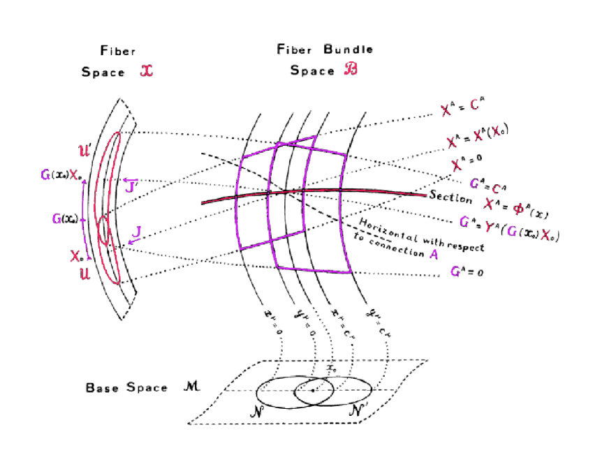
Figure 1: Schematic representation showing two-dimensional subspaces of a (curved) fibre space ${\color[rgb]{1,0,0}{\cal X}}$, a base space ${\cal M}$, and a bundle ${\color[rgb]{1,0,0}{\cal B}}$ with fibre ${\color[rgb]{1,0,0}{\cal X}}$ over ${\cal M}$, indicating the relationships between the various local coordinate patches mentioned in the text, and showing the distinction between the original gauge projection ${\color[rgb]{.66,0,.33}{J}}$ determined (for ${\color[rgb]{1,0,0}{X}}\in{\color[rgb]{1,0,0}{\cal X}}$, $x\in{\cal M})$ in the form ${\color[rgb]{.66,0,.33}{J}}\{{\color[rgb]{1,0,0}{X}},x\}={\color[rgb]{1,0,0}{X}}$ by the local product structure corresponding to some initially given gauge over a neighbourhood ${\cal N}\subset{\cal M}$, and a new gauge projection ${\color[rgb]{.66,0,.33}{J}}^{\prime}$ over ${\cal N}^{\prime}$ given in terms of the initial local product structure over the intersection ${\cal N}\cap{\cal N}^{\prime}$ by ${\color[rgb]{.66,0,.33}{J}}^{\prime}\{{\color[rgb]{1,0,0}{X}},x\}={\color[rgb]{.66,0,.33}{G}}\{x\}{\color[rgb]{1,0,0}{X}}$. (The positions of thepatches ${\cal N}$, ${\cal N}^{\prime}$, in ${\cal M}$ and ${\cal U}$, ${\cal U}^{\prime}$, in ${{\color[rgb]{1,0,0}{\cal X}}}$ are indicated by pairs of points representing the coordinate origin and some other arbitrary constant values denoted by the letter c.) .

In the simple vector bundles that are most commonly used in physics, the algebra ${\color[rgb]{.66,0,.33}{\cal A}}$ can conveniently be represented in terms of matrices, but in the general nonlinear case it is more useful to think of the algebra as represented by the vector fields that generate the corresponding infinitesimal diffeomorphisms on the primary fibre space ${\color[rgb]{1,0,0}{\cal X}}$ under consideration. The basic function of a gauge field ${\color[rgb]{.66,0,.33}\bf{A}}$ is to determine, for any infinitesimal base displacement ${\rm d}x$, a corresponding algebra element

$${\color[rgb]{.66,0,.33}\bf{a}}={\color[rgb]{.66,0,.33}\bf{A}}_{\mu}\,{\rm d}x^{\mu}$$ (40)

which will be realised by a corresponding fibre vector field with components

$${\color[rgb]{.66,0,.33}{a}}^{{}_{\color[rgb]{1,0,0}{A}}}={\color[rgb]{.66,0,.33}{A}}_{\mu}^{\ {}_{\color[rgb]{1,0,0}{A}}}\,{\rm d}x^{\mu}\,.$$ (41)

The role of this vector field is to determine the (infinitesimal) deflection between the horizontal projection, as determined by the local direct product structure associated with the gauge patch under consideration (in effect the local coordinates $\{{\color[rgb]{1,0,0}{X}},x\}$) between fibres over base points differing by the infinitesimal base displacement ${\rm d}x$, and the corresponding horizontal projection as determined by the connection.

The specification of a connection in this way enables one to define a gauge covariant vertical displacement $\hbox to0.0pt{\raise 4.0pt\hbox{\color[rgb]{1,0,0}{\,\bf-}}\hss}{\rm d}{\color[rgb]{1,0,0}{X}}$ between neighboring points on neighboring fibres, as determined with respect to horizontality as specified by the connection. The components of the covariant vertical displacement may be evaluated as the difference,

$$\hbox to0.0pt{\raise 4.0pt\hbox{\color[rgb]{1,0,0}{\,\bf-}}\hss}{\rm d}{\color[rgb]{1,0,0}{X}}^{{}_{\color[rgb]{1,0,0}{A}}}={\rm d}{\color[rgb]{1,0,0}{X}}^{{}_{\color[rgb]{1,0,0}{A}}}-{\rm d}_{\color[rgb]{.66,0,.33}\bf{a}}{\color[rgb]{1,0,0}{X}}^{{}_{\color[rgb]{1,0,0}{A}}}$$ (42)

between the vertical deviation ${\rm d}{\color[rgb]{1,0,0}{X}}^{{}_{\color[rgb]{1,0,0}{A}}}$ determined by the local coordinates (i.e. by the local product structure of the gauge path) and the vertical deviation

$${\rm d}_{\color[rgb]{.66,0,.33}\bf{a}}{\color[rgb]{1,0,0}{X}}^{{}_{\color[rgb]{1,0,0}{A}}}=-{\color[rgb]{.66,0,.33}{a}}^{{}_{\color[rgb]{1,0,0}{A}}}$$ (43)

between horizontality with respect to the connection and horizontality as determined by the local coordinates. Hence if we are considering a section ${\color[rgb]{1,0,0}{\Phi}}$, substitution of the corresponding coordinate displacement formula

$${\rm d}{\color[rgb]{1,0,0}{X}}^{{}_{\color[rgb]{1,0,0}{A}}}={\color[rgb]{1,0,0}{X}}^{{}_{\color[rgb]{1,0,0}{A}}}_{\ \mu}\,{\rm d}x^{\mu}$$ (44)

into (42) gives the expression

$$\hbox to0.0pt{\raise 4.0pt\hbox{\color[rgb]{1,0,0}{\,\bf-}}\hss}{\rm d}{\color[rgb]{1,0,0}{X}}^{{}_{\color[rgb]{1,0,0}{A}}}=({\color[rgb]{1,0,0}{X}}^{{}_{\color[rgb]{1,0,0}{A}}}_{\ \mu}+{\color[rgb]{.66,0,.33}{A}}^{{}_{\color[rgb]{1,0,0}{A}}}_{\ \mu})\,{\rm d}x^{\mu}$$ (45)

for the corresponding covariant displacement components, where ${\color[rgb]{1,0,0}{X}}^{{}_{\color[rgb]{1,0,0}{A}}}_{\ \mu}$ are the tangent projection components associated with the section ${\color[rgb]{1,0,0}{\Phi}}$ as given by (23). (See Fig. 1.)

It is evident that the quantity $\hbox to0.0pt{\raise 4.0pt\hbox{\color[rgb]{1,0,0}{\,\bf-}}\hss}{\rm d}{\color[rgb]{1,0,0}{X}}^{{}_{\color[rgb]{1,0,0}{A}}}$ constructed in this way will be vectorially covariant under the effect of a general (base-position dependent) fibre-coordinate transformation of the form (7) which gives

$${\rm d}{\color[rgb]{1,0,0}{X}}^{{}_{\color[rgb]{1,0,0}{A}}}\ \mapsto\ {\color[rgb]{.66,0,.33}{G}}^{{}_{\color[rgb]{1,0,0}{A}}}_{\ {}_{\color[rgb]{1,0,0}{B}}}\,{\rm d}{\color[rgb]{1,0,0}{X}}^{{}_{\color[rgb]{1,0,0}{B}}}+{\color[rgb]{.66,0,.33}{G}}^{{}_{\color[rgb]{1,0,0}{A}}}_{\ ,\mu}\,{\rm d}x^{\mu}$$ (46)

provided that the gauge connection field ${\color[rgb]{.66,0,.33}\bf{A}}$ undergoes the corresponding transformation, which will be given explicitly for the vector realization by

$${\color[rgb]{.66,0,.33}{A}}_{\mu}^{\ {}_{\color[rgb]{1,0,0}{A}}}\ \mapsto\ {\color[rgb]{.66,0,.33}{G}}^{{}_{\color[rgb]{1,0,0}{A}}}_{\ {}_{\color[rgb]{1,0,0}{B}}}{\color[rgb]{.66,0,.33}{A}}_{\mu}^{\ {}_{\color[rgb]{1,0,0}{B}}}-{\color[rgb]{.66,0,.33}{G}}^{{}_{\color[rgb]{1,0,0}{A}}}_{\ ,\mu}$$ (47)

since the inhomogeneous terms will cancel so as to give the purely vectorial covariance rule

$$\hbox to0.0pt{\raise 4.0pt\hbox{\color[rgb]{1,0,0}{\,\bf-}}\hss}{\rm d}{\color[rgb]{1,0,0}{X}}^{{}_{\color[rgb]{1,0,0}{A}}}\ \mapsto{\color[rgb]{.66,0,.33}{G}}^{{}_{\color[rgb]{1,0,0}{A}}}_{\ {}_{\color[rgb]{1,0,0}{B}}}\,\hbox to0.0pt{\raise 4.0pt\hbox{\color[rgb]{1,0,0}{\,\bf-}}\hss}{\rm d}{\color[rgb]{1,0,0}{X}}^{{}_{\color[rgb]{1,0,0}{B}}}\,.$$ (48)

By a rather longer calculation one can also verify that (7) and (47) also imply an analogous purely vectorial covariance rule

$${\color[rgb]{.66,0,.33}F}_{\!\mu\nu}^{\ \ {}_{\color[rgb]{1,0,0}{A}}}\ \mapsto{\color[rgb]{.66,0,.33}{G}}^{{}_{\color[rgb]{1,0,0}{A}}}_{\ {}_{\color[rgb]{1,0,0}{B}}}\,{\color[rgb]{.66,0,.33}F}_{\!\mu\nu}^{\ \ {}_{\color[rgb]{1,0,0}{B}}}$$ (49)

for the components of the vector realisation of the gauge curvature ${\color[rgb]{.66,0,.33}\bf{F}}$, as defined by

$${\color[rgb]{.66,0,.33}F}_{\!\mu\nu}^{\ \ {}_{\color[rgb]{1,0,0}{A}}}={\color[rgb]{.66,0,.33}F}_{\!\mu\nu}^{\ \ {\color[rgb]{.66,0,.33}\alpha}}\,{\color[rgb]{.66,0,.33}{a}}_{\color[rgb]{.66,0,.33}\alpha}^{\,{}_{\color[rgb]{1,0,0}{A}}}\,$$ (50)

where ${\color[rgb]{.66,0,.33}{a}}_{\color[rgb]{.66,0,.33}\alpha}^{\,{}_{\color[rgb]{1,0,0}{A}}}$ are the components of the vector realization of ${\color[rgb]{.66,0,.33}\bf{a}}_{\color[rgb]{.66,0,.33}\alpha}$, and the basis components ${\color[rgb]{.66,0,.33}F}_{\!\mu\nu}^{\ \ {\color[rgb]{.66,0,.33}\alpha}}$ of the gauge curvature are specified by (39).

Since the algebra commutator relations will be realised by the Lie differentiation commutator of the vector fields on ${\color[rgb]{1,0,0}{\cal X}}$, the structure relations (37) will be realised concretely by

$$2{\color[rgb]{.66,0,.33}{a}}_{[{\color[rgb]{.66,0,.33}\alpha}|\,,_{\color[rgb]{1,0,0}{B}}}^{\ \ {}_{\color[rgb]{1,0,0}{A}}}{\color[rgb]{.66,0,.33}{a}}_{|{\color[rgb]{.66,0,.33}\beta}]}^{\,\ {}_{\color[rgb]{1,0,0}{B}}}={\color[rgb]{.66,0,.33}{\copyright}}_{{\color[rgb]{.66,0,.33}\alpha}{\color[rgb]{.66,0,.33}\beta}}^{\,\ \ {\color[rgb]{.66,0,.33}\gamma}}\,{\color[rgb]{.66,0,.33}{a}}_{\color[rgb]{.66,0,.33}\gamma}^{\,{}_{\color[rgb]{1,0,0}{A}}}\,.$$ (51)

Hence by substitution in (39) we obtain an explicit, Lie algebra-basis independent, expression for the components ${\color[rgb]{.66,0,.33}F}_{\!\mu\nu}^{\ \ {}_{\color[rgb]{1,0,0}{A}}}$ of the realization of the gauge curvature ${\color[rgb]{.66,0,.33}\bf{F}}$, namely

$${\color[rgb]{.66,0,.33}F}_{\!\mu\nu}^{\ \ {}_{\color[rgb]{1,0,0}{A}}}=2{\color[rgb]{.66,0,.33}{A}}_{[\nu\,\ ,\,\mu]}^{\ \ {}_{\color[rgb]{1,0,0}{A}}}+2{\color[rgb]{.66,0,.33}{A}}_{[\nu}^{\,\ {}_{\color[rgb]{1,0,0}{B}}}{\color[rgb]{.66,0,.33}{A}}_{\mu]\ ,_{\color[rgb]{1,0,0}{B}}}^{\,\ {}_{\color[rgb]{1,0,0}{A}}}\,.$$ (52)

It is an essentially straightforward exercise in partial differentiation to verify directly that this fundamental primary bundle realisation of the gauge curvature does indeed undergo a transformation of the vectorial form (49) under the effect of a general gauge-patch transformation as specified by (7) and (48). This establishes that the base-space two-form valued vertical (i.e. fibre-space tangent) vector field ${\color[rgb]{.66,0,.33}\bf{F}}$ specified by (49) is globally well defined over the whole of the primary bundle ${\color[rgb]{1,0,0}{\cal B}}$, unlike the base space one-form valued vertical vector field ${\color[rgb]{.66,0,.33}\bf{A}}$ which is gauge patch dependent.

The property of existing as a field over the whole of the primary bundle ${\color[rgb]{1,0,0}{\cal B}}$ distinguishes the primary gauge-curvature realisation ${\color[rgb]{.66,0,.33}\bf{F}}$ from the other bitensorial entities introduced in the previous sections, which were defined only over some particular section ${\color[rgb]{1,0,0}{\Phi}}$ in ${\color[rgb]{1,0,0}{\cal B}}$. In dealing with entities such as ${\color[rgb]{.66,0,.33}\bf{F}}$ and ${\color[rgb]{.66,0,.33}\bf{A}}$ which are defined over the whole of the fibres and not just at the section ${\color[rgb]{1,0,0}{\Phi}}$, one must take care to distinguish the partial component derivatives, indicated by a comma, from the total base-space gradient components for the field over ${\cal M}$ that would be determined by the section ${\color[rgb]{1,0,0}{\Phi}}$. Thus although we could use the expressions $\partial_{\mu}{\color[rgb]{.66,0,.33}{A}}_{\nu}^{\ {\color[rgb]{.66,0,.33}\alpha}}$ and ${\color[rgb]{.66,0,.33}{A}}_{\nu\ ,\,\mu}^{\ {\color[rgb]{.66,0,.33}\alpha}}$ interchangeably in (39), it is important to notice that $\partial_{\mu}{\color[rgb]{.66,0,.33}{A}}_{\nu}^{\ {}_{\color[rgb]{1,0,0}{A}}}$ is not the same as ${\color[rgb]{.66,0,.33}{A}}_{\nu\ ,\,\mu}^{\ {}_{\color[rgb]{1,0,0}{A}}}$ in the algebra-basis independent expression (52), the distinction being specified as a function of the section ${\color[rgb]{1,0,0}{\Phi}}$ by

$$\partial_{\mu}{\color[rgb]{.66,0,.33}{A}}_{\nu}^{\ {}_{\color[rgb]{1,0,0}{A}}}={\color[rgb]{.66,0,.33}{A}}_{\nu\ ,\,\mu}^{\ {}_{\color[rgb]{1,0,0}{A}}}+{\color[rgb]{.66,0,.33}{A}}_{\nu\ ,_{\color[rgb]{1,0,0}{B}}}^{\ {}_{\color[rgb]{1,0,0}{A}}}{\color[rgb]{1,0,0}{X}}^{{}_{\color[rgb]{1,0,0}{B}}}_{\ \mu}\,.$$ (53)

By paying attention to this distinction, it will be possible to work with an explicit, but Lie algebra-basis independent notation scheme throughout the remainder of this work, thereby avoiding any further reference to such cumbersome paraphenalia as the structure constants.

Up to this point we have made no reference to any specific properties of the gauge group ${\color[rgb]{.66,0,.33}{\cal G}}$: the analysis in this section would be valid for transformations ${\color[rgb]{1,0,0}{X}}^{{}_{\color[rgb]{1,0,0}{A}}}\mapsto{\color[rgb]{.66,0,.33}{G}}^{{}_{\color[rgb]{1,0,0}{A}}}$ resulting from the general action of the entire (infinite parameter) group of diffeomorphisms on the fibre space ${\color[rgb]{1,0,0}{\cal X}}$. However, for the purpose of constructing a gauge covariant differentiation formalism, as will be done in the section that follows, it will be necessary to restrict ourselves to situations for which ${\color[rgb]{.66,0,.33}{\cal G}}$ is included in the at most finite-dimensional diffeomorphism subgroup leaving the chosen fibre-space connection $\hat{\color[rgb]{1,0,0}{\Gamma}}$ invariant.

5 Gauge-covariant bitensorial differentiation

It is immediately evident from the work of the previous section that for any section ${\color[rgb]{1,0,0}{\Phi}}\{x\}$ in the primary bundle ${\color[rgb]{1,0,0}{\cal B}}$ the gauge connection ${\color[rgb]{.66,0,.33}\bf{A}}$ will determine a well defined covariant vector field ${\color[rgb]{.66,0,.33}{D}}\Phi$ over the base-space ${\cal M}$, whose components can be read out from the expression

$$\hbox to0.0pt{\raise 4.0pt\hbox{\color[rgb]{1,0,0}{\,\bf-}}\hss}{\rm d}{\color[rgb]{1,0,0}{X}}^{{}_{\color[rgb]{1,0,0}{A}}}={\color[rgb]{1,0,0}{\Phi}}^{{}_{\color[rgb]{1,0,0}{A}}}_{\ {\color[rgb]{.66,0,.33}{|\!\!|\!\!|}}\,\mu}\,{\rm d}x^{\mu}$$ (54)

for the covariant vertical displacement $\hbox to0.0pt{\raise 4.0pt\hbox{\color[rgb]{1,0,0}{\,\bf-}}\hss}{\rm d}{\color[rgb]{1,0,0}{X}}$ resulting from a base-space displacement ${\rm d}x$, where we have intrioduced a heavy bar notation convention

$${\color[rgb]{.66,0,.33}{D}}_{\mu}{\color[rgb]{1,0,0}{\Phi}}^{{}_{\color[rgb]{1,0,0}{A}}}={\color[rgb]{1,0,0}{\Phi}}^{{}_{\color[rgb]{1,0,0}{A}}}_{\ {\color[rgb]{.66,0,.33}{|\!\!|\!\!|}}\,\mu}$$ (55)

for gauge-covariant differentiation. Recalling our previous abbreviation

$$\partial_{\mu}{\color[rgb]{1,0,0}{\Phi}}^{{}_{\color[rgb]{1,0,0}{A}}}={\color[rgb]{1,0,0}{X}}^{{}_{\color[rgb]{1,0,0}{A}}}_{\ \mu}$$ (56)

we immediately obtain the compact expression

$${\color[rgb]{1,0,0}{\Phi}}^{{}_{\color[rgb]{1,0,0}{A}}}_{\ {\color[rgb]{.66,0,.33}{|\!\!|\!\!|}}\,\mu}={\color[rgb]{1,0,0}{X}}^{{}_{\color[rgb]{1,0,0}{A}}}_{\ \mu}+{\color[rgb]{.66,0,.33}{A}}_{\mu}^{\ {}_{\color[rgb]{1,0,0}{A}}}$$ (57)

for the bitensorial derivative components ${\color[rgb]{1,0,0}{\Phi}}^{{}_{\color[rgb]{1,0,0}{A}}}_{\ {\color[rgb]{.66,0,.33}{|\!\!|\!\!|}}\,\mu}$ by substituting (45) in (54).

This lowest order differentiation procedure obviously does not depend on the specification of any intrinsic structure on the fibre ${\color[rgb]{1,0,0}{\cal X}}$ or base ${\cal M}$ of ${\color[rgb]{1,0,0}{\cal B}}$. However, in order to go on (analogously to the work of Sec. 3) to the construction of higher order bitensorial derivatives, the reintroduction of the fibre connection $\hat{\color[rgb]{1,0,0}{\Gamma}}$ on ${\color[rgb]{1,0,0}{\cal X}}$ and, more routinely, of the base connection ${\color[rgb]{0,0,.66}\Gamma}$ on ${\cal M}$, will evidently be necessary.

Before continuing, we now make the usual supposition that the gauge group ${\color[rgb]{.66,0,.33}{\cal G}}$ acting effectively on the primary bundle ${\color[rgb]{1,0,0}{\cal B}}$ should be restricted so as to consist only of fibre isomorphisms, i.e. that it should leave invariant all relevant structure on the fibre space ${\color[rgb]{1,0,0}{\cal X}}$ in which the primary field is evaluated. As a minimal requirement we must at least demand that the transformation group ${\color[rgb]{.66,0,.33}{\cal G}}$ should preserve the only structure that has been introduced so far on ${\color[rgb]{1,0,0}{\cal X}}$, namely the indispensible fibre connection $\hat{\color[rgb]{1,0,0}{\Gamma}}$; i.e. the gauge transformations must be restricted so as not to violate the essential property

$$\hat{\color[rgb]{1,0,0}{\Gamma}}{{}_{\!{}_{\color[rgb]{1,0,0}{A}}\ {}_{\color[rgb]{1,0,0}{C}}\,,\,\mu}^{\ {}_{\color[rgb]{1,0,0}{B}}}}=0$$ (58)

characterising any allowable local gauge coordinate system $\{{\color[rgb]{1,0,0}{X}},x\}$. In order to express the corresponding restiction on the gauge algebra, it is convenient, following Yano[5], to introduce an abbreviation, which we shall indicate by a subscript colon, to indicate a covariant derivative of a vector field that differs from the usual one in that the connection is inserted the wrong way round. Thus for the particular case of the gauge vector one form ${\color[rgb]{.66,0,.33}\bf{A}}$ we introduce a corresponding gauge tensor one form ${\color[rgb]{.66,0,.33}\bf{A}}_{:}$ defined by

$${\color[rgb]{.66,0,.33}{A}}_{\mu\ :_{\color[rgb]{1,0,0}{B}}}^{\ {}_{\color[rgb]{1,0,0}{A}}}={\color[rgb]{.66,0,.33}{A}}_{\mu\ ,_{\color[rgb]{1,0,0}{B}}}^{\ {}_{\color[rgb]{1,0,0}{A}}}+{\color[rgb]{.66,0,.33}{A}}_{\mu}^{\ {}_{\color[rgb]{1,0,0}{C}}}\,\hat{\color[rgb]{1,0,0}{\Gamma}}{{}_{\!{}_{\color[rgb]{1,0,0}{C}}\ {}_{\color[rgb]{1,0,0}{B}}}^{\ {}_{\color[rgb]{1,0,0}{A}}}}$$ (59)

or equivalently

$${\color[rgb]{.66,0,.33}{A}}_{\mu\ :_{\color[rgb]{1,0,0}{B}}}^{\ {}_{\color[rgb]{1,0,0}{A}}}=\hat{\color[rgb]{1,0,0}{\nabla}}_{\!{}_{\color[rgb]{1,0,0}{B}}}{\color[rgb]{.66,0,.33}{A}}_{\mu}^{\ {}_{\color[rgb]{1,0,0}{A}}}+{\color[rgb]{.66,0,.33}{A}}_{\mu}^{\ {}_{\color[rgb]{1,0,0}{C}}}\,\hat{\color[rgb]{1,0,0}{\Theta}}{{}_{\!{}_{{\color[rgb]{1,0,0}{C}}{\color[rgb]{1,0,0}{B}}}}^{\ \ {}_{\color[rgb]{1,0,0}{A}}}}\,,$$ (60)

where $\hat{\color[rgb]{1,0,0}{\nabla}}$ denotes the ordinary operation of covariant differentiation along the fibres with respect to the fibre connection $\hat{\color[rgb]{1,0,0}{\Gamma}}$. In the absence of the torsion $\hat{\color[rgb]{1,0,0}{\Theta}}$ the distinction between this Yano covariant derivative and the ordinary covariant derivative disappears. In terms of this notation, the essential requirement that the fibre connection be invariant under the action generated by the primary gauge field ${\color[rgb]{.66,0,.33}\bf{A}}$ can be obtained (from Yano’s formula [5] for the Lie derivative of the connection) in the form

$$\hat{\color[rgb]{1,0,0}{\nabla}}_{\!{}_{\color[rgb]{1,0,0}{B}}}{\color[rgb]{.66,0,.33}{A}}_{\mu\ :_{\color[rgb]{1,0,0}{C}}}^{\ {}_{\color[rgb]{1,0,0}{A}}}={\color[rgb]{.66,0,.33}{A}}_{\mu}^{\ {}_{\color[rgb]{1,0,0}{D}}}\,\hat{\color[rgb]{1,0,0}{R}}{{}_{{}_{{\color[rgb]{1,0,0}{B}}{\color[rgb]{1,0,0}{D}}}\ {}_{\color[rgb]{1,0,0}{C}}}^{\ \ \ {}_{\color[rgb]{1,0,0}{A}}}}$$ (61)

This basic postulate includes, as a consequence, the corresponding decoupled invariance requirement for the torsion tensor, i.e.

$${\color[rgb]{.66,0,.33}{A}}_{\mu}^{\ {}_{\color[rgb]{1,0,0}{D}}}\hat{\color[rgb]{1,0,0}{\nabla}}_{\!{}_{\color[rgb]{1,0,0}{D}}}\hat{\color[rgb]{1,0,0}{\Theta}}{{}_{\!{}_{{\color[rgb]{1,0,0}{B}}{\color[rgb]{1,0,0}{C}}}}^{\ \ {}_{\color[rgb]{1,0,0}{A}}}}={\color[rgb]{.66,0,.33}{A}}_{\mu\ :_{\color[rgb]{1,0,0}{D}}}^{\ {}_{\color[rgb]{1,0,0}{A}}}\hat{\color[rgb]{1,0,0}{\Theta}}{{}_{\!{}_{{\color[rgb]{1,0,0}{B}}{\color[rgb]{1,0,0}{C}}}}^{\,\ \ {}_{\color[rgb]{1,0,0}{D}}}}+2{\color[rgb]{.66,0,.33}{A}}_{\mu\ :[_{\color[rgb]{1,0,0}{C}}|}^{\ {}_{\color[rgb]{1,0,0}{D}}}\hat{\color[rgb]{1,0,0}{\Theta}}{{}_{\!{}_{{\color[rgb]{1,0,0}{D}}}|_{\color[rgb]{1,0,0}{B}}]}^{\,\ \ \ {}_{\color[rgb]{1,0,0}{A}}}}\,.$$ (62)

For purely base-tensorial entities the question of gauge invariance does not arise. We therefor proceed directly to consider the appropriate gauge-covariant generalization of the definition (17) of the absolute variation of the simplest kind of fibre-tensorial quantity, an ordinary vector ${\color[rgb]{1,0,0}{V}}$, between nearby points in nearby fibres separated by a base displacement ${\rm d}x$. Evidently the required gauge-covariant variation $\hbox to0.0pt{\raise 4.0pt\hbox{\color[rgb]{1,0,0}{\,\bf-}}\hss}{\rm d}{\color[rgb]{1,0,0}{V}}$ should be defined as the covariant variation with respect to the fibre connection $\hat{\color[rgb]{1,0,0}{\Gamma}}$ along the vertical displacement $\hbox to0.0pt{\raise 4.0pt\hbox{\color[rgb]{1,0,0}{\,\bf-}}\hss}{\rm d}{\color[rgb]{1,0,0}{X}}$ as specified by the projection that is horizontal with respect to the gauge connection. This means that we must take

$$\hbox to0.0pt{\raise 4.0pt\hbox{\color[rgb]{1,0,0}{\,\bf-}}\hss}{\rm d}{\color[rgb]{1,0,0}{V}}^{{}_{\color[rgb]{1,0,0}{A}}}={\rm d}({\color[rgb]{1,0,0}{V}}^{{}_{\color[rgb]{1,0,0}{A}}})-{\rm d}_{{\color[rgb]{.66,0,.33}\bf{a}}}{\color[rgb]{1,0,0}{V}}^{{}_{\color[rgb]{1,0,0}{A}}}+(\hbox to0.0pt{\raise 4.0pt\hbox{\color[rgb]{1,0,0}{\,\bf-}}\hss}{\rm d}{\color[rgb]{1,0,0}{X}}^{{}_{\color[rgb]{1,0,0}{B}}})\,\hat{\color[rgb]{1,0,0}{\Gamma}}{{}_{\!{}_{\color[rgb]{1,0,0}{B}}\ {}_{\color[rgb]{1,0,0}{C}}}^{\ {}_{\color[rgb]{1,0,0}{A}}}}{\color[rgb]{1,0,0}{V}}^{{}_{\color[rgb]{1,0,0}{C}}}\,,$$ (63)

where $\hbox to0.0pt{\raise 4.0pt\hbox{\color[rgb]{1,0,0}{\,\bf-}}\hss}{\rm d}{\color[rgb]{1,0,0}{X}}^{{}_{\color[rgb]{1,0,0}{A}}}$ are the components of the covariant veritical displacement as specified by (42), or more explicitely (45), and ${\rm d}_{{\color[rgb]{.66,0,.33}\bf{a}}}{\color[rgb]{1,0,0}{V}}^{{}_{\color[rgb]{1,0,0}{A}}}$ are the vector component variations resulting from the fact that horizontality with respect to the local fibre coordinates ${\color[rgb]{1,0,0}{X}}^{{}_{\color[rgb]{1,0,0}{A}}}$ differs from horizontality with respect to the gauge connection by the effect of the infinitesimal Lie displacement induced by the vector field ${\color[rgb]{.66,0,.33}\bf{a}}$ specified on the fibre by (41), which gives

$${\rm d}_{{\color[rgb]{.66,0,.33}\bf{a}}}{\color[rgb]{1,0,0}{V}}^{{}_{\color[rgb]{1,0,0}{A}}}=-{\color[rgb]{.66,0,.33}{a}}^{{}_{\color[rgb]{1,0,0}{A}}}_{\ ,_{\color[rgb]{1,0,0}{B}}}{\color[rgb]{1,0,0}{V}}^{{}_{\color[rgb]{1,0,0}{B}}}\,.$$ (64)

Thus explicitly we shall have

$$\hbox to0.0pt{\raise 4.0pt\hbox{\color[rgb]{1,0,0}{\,\bf-}}\hss}{\rm d}{\color[rgb]{1,0,0}{V}}^{{}_{\color[rgb]{1,0,0}{A}}}={\rm d}({\color[rgb]{1,0,0}{V}}^{{}_{\color[rgb]{1,0,0}{A}}})+\left[{\color[rgb]{.66,0,.33}{A}}_{\mu\ ,_{\color[rgb]{1,0,0}{B}}}^{\ {}_{\color[rgb]{1,0,0}{A}}}{\rm d}x^{\mu}+({\color[rgb]{.66,0,.33}{A}}_{\mu}^{\ {}_{\color[rgb]{1,0,0}{C}}}\,{\rm d}x^{\mu}+{\rm d}{\color[rgb]{1,0,0}{X}}^{{}_{\color[rgb]{1,0,0}{C}}})\hat{\color[rgb]{1,0,0}{\Gamma}}{{}_{\!{}_{\color[rgb]{1,0,0}{C}}\ {}_{\color[rgb]{1,0,0}{B}}}^{\ {}_{\color[rgb]{1,0,0}{A}}}}\right]{\color[rgb]{1,0,0}{V}}^{{}_{\color[rgb]{1,0,0}{B}}}\,.$$ (65)

In the case where ${\color[rgb]{1,0,0}{V}}$ is a tangent vector defined as a field on a section ${\color[rgb]{1,0,0}{\Phi}}\{x\}$, there will be a corresponding bitensorial covariant derivative which can be read out from the defining formula

$$\hbox to0.0pt{\raise 4.0pt\hbox{\color[rgb]{1,0,0}{\,\bf-}}\hss}{\rm d}{\color[rgb]{1,0,0}{V}}^{{}_{\color[rgb]{1,0,0}{A}}}={\color[rgb]{1,0,0}{V}}^{{}_{\color[rgb]{1,0,0}{A}}}_{\ {\color[rgb]{.66,0,.33}{|\!\!|\!\!|}}\,\mu}\,{\rm d}x^{\mu}$$ (66)

using the abbreviated bar suffix notation system

$${\color[rgb]{.66,0,.33}{D}}_{\mu}{\color[rgb]{1,0,0}{V}}^{{}_{\color[rgb]{1,0,0}{A}}}={\color[rgb]{1,0,0}{V}}^{{}_{\color[rgb]{1,0,0}{A}}}_{\ {\color[rgb]{.66,0,.33}{|\!\!|\!\!|}}\,\mu}\,.$$ (67)

Thus we obtain the covariant derivative components in the form

$${\color[rgb]{1,0,0}{V}}^{{}_{\color[rgb]{1,0,0}{A}}}_{\ {\color[rgb]{.66,0,.33}{|\!\!|\!\!|}}\,\mu}=\partial_{\mu}{\color[rgb]{1,0,0}{V}}^{{}_{\color[rgb]{1,0,0}{A}}}+{\color[rgb]{.66,0,.33}\omega}_{\mu\ _{\color[rgb]{1,0,0}{B}}}^{\ {}_{\color[rgb]{1,0,0}{A}}}{\color[rgb]{1,0,0}{V}}^{{}_{\color[rgb]{1,0,0}{B}}}\,,$$ (68)

where the section dependent connector ${\color[rgb]{.66,0,.33}\omega}$ [as introduced in (4)] will be given, using the notation of (57), by

$${\color[rgb]{.66,0,.33}\omega}_{\mu\ _{\color[rgb]{1,0,0}{B}}}^{\ {}_{\color[rgb]{1,0,0}{A}}}={\color[rgb]{1,0,0}{\Phi}}^{{}_{\color[rgb]{1,0,0}{C}}}_{\ {\color[rgb]{.66,0,.33}{|\!\!|\!\!|}}\,\mu}\hat{\color[rgb]{1,0,0}{\Gamma}}{{}_{\!{}_{\color[rgb]{1,0,0}{C}}\ {}_{\color[rgb]{1,0,0}{B}}}^{\ {}_{\color[rgb]{1,0,0}{A}}}}+{\color[rgb]{.66,0,.33}{A}}_{\mu\ ,_{\color[rgb]{1,0,0}{B}}}^{\ {}_{\color[rgb]{1,0,0}{A}}}$$ (69)

or equivalently, using the notation of (22) and (59),

$${\color[rgb]{.66,0,.33}\omega}_{\mu\ _{\color[rgb]{1,0,0}{B}}}^{\ {}_{\color[rgb]{1,0,0}{A}}}={\color[rgb]{1,0,0}{\Gamma}}_{\!\mu\ _{\color[rgb]{1,0,0}{B}}}^{\ {}_{\color[rgb]{1,0,0}{A}}}+{\color[rgb]{.66,0,.33}{A}}_{\mu\ :_{\color[rgb]{1,0,0}{B}}}^{\ {}_{\color[rgb]{1,0,0}{A}}}\,.$$ (70)

Having thus obtained the required connector ${\color[rgb]{.66,0,.33}\omega}$ that is needed for covariant differentiation of a simple fibre vector on the section, one can go on immediately in the usual way to construct the corresponding covariant derivatives of more general fibre-tensorial and bitensorial quantities by adding an appropriate connector term for each index (a term involving ${\color[rgb]{.66,0,.33}\omega}_{\mu\ _{\color[rgb]{1,0,0}{B}}}^{\ {}_{\color[rgb]{1,0,0}{A}}}$ with a positive or negative sign for each respectively contravariant or covariant fibre index,and similarly a term involving ${\color[rgb]{0,0,.66}\Gamma}_{\!\mu\ \rho}^{\ \nu}$ for each base-space index.

The resulting generalisation of the derivative commutator rule (28) for the primary section ${\color[rgb]{1,0,0}{\Phi}}$ itself involves the fibre and base torsions and the gauge curvature, taking the form

$$2{\color[rgb]{1,0,0}{\Phi}}^{{}_{\color[rgb]{1,0,0}{A}}}_{\ {\color[rgb]{.66,0,.33}{|\!\!|\!\!|}}\,[\nu\,{\color[rgb]{.66,0,.33}{|\!\!|\!\!|}}\,\mu]}={\color[rgb]{1,0,0}{\Phi}}^{{}_{\color[rgb]{1,0,0}{C}}}_{\ {\color[rgb]{.66,0,.33}{|\!\!|\!\!|}}\,\mu}{\color[rgb]{1,0,0}{\Phi}}^{{}_{\color[rgb]{1,0,0}{D}}}_{\ {\color[rgb]{.66,0,.33}{|\!\!|\!\!|}}\,\nu}\,\hat{\color[rgb]{1,0,0}{\Theta}}{{}_{{}_{{\color[rgb]{1,0,0}{C}}{\color[rgb]{1,0,0}{D}}}}^{\ \ \ {}_{\color[rgb]{1,0,0}{A}}}}-{\color[rgb]{0,0,.66}{\Theta}}_{\mu\nu}^{\,\ \ \rho}\,{\color[rgb]{1,0,0}{\Phi}}^{{}_{\color[rgb]{1,0,0}{A}}}_{\ {\color[rgb]{.66,0,.33}{|\!\!|\!\!|}}\,\rho}+{\color[rgb]{.66,0,.33}F}_{\!\mu\nu}^{\ \ {}_{\color[rgb]{1,0,0}{A}}}\,.$$ (71)

The analogous commutator rule, generalising (30), for a fibre vector field over the section ${\color[rgb]{1,0,0}{\Phi}}$ involves the fibre curvature and the gauge curvature as well as the base torsion, taking the form

$$2{\color[rgb]{1,0,0}{V}}^{{}_{\color[rgb]{1,0,0}{A}}}_{\ {\color[rgb]{.66,0,.33}{|\!\!|\!\!|}}\,[\nu\,{\color[rgb]{.66,0,.33}{|\!\!|\!\!|}}\,\mu]}={\color[rgb]{.66,0,.33}\Omega}_{\mu\nu\ _{\color[rgb]{1,0,0}{B}}}^{\,\ \ {}_{\color[rgb]{1,0,0}{A}}}{\color[rgb]{1,0,0}{V}}^{{}_{\color[rgb]{1,0,0}{B}}}-{\color[rgb]{0,0,.66}{\Theta}}_{\mu\nu}^{\,\ \ \rho}\,{\color[rgb]{1,0,0}{V}}^{{}_{\color[rgb]{1,0,0}{A}}}_{\ {\color[rgb]{.66,0,.33}{|\!\!|\!\!|}}\,\rho}\,,$$ (72)

where the total curvature, as defined by (11), can be evaluated, (using (61) and (52), as the sum of two separately bitensorially covariant terms, in the form

$${\color[rgb]{.66,0,.33}\Omega}_{\mu\nu\ _{\color[rgb]{1,0,0}{B}}}^{\,\ \ {}_{\color[rgb]{1,0,0}{A}}}={\color[rgb]{1,0,0}{\Phi}}^{{}_{\color[rgb]{1,0,0}{C}}}_{\ {\color[rgb]{.66,0,.33}{|\!\!|\!\!|}}\,\mu}{\color[rgb]{1,0,0}{\Phi}}^{{}_{\color[rgb]{1,0,0}{D}}}_{\ {\color[rgb]{.66,0,.33}{|\!\!|\!\!|}}\,\nu}\,\hat{\color[rgb]{1,0,0}{R}}{{}_{{}_{{\color[rgb]{1,0,0}{C}}{\color[rgb]{1,0,0}{D}}}\ {}_{\color[rgb]{1,0,0}{B}}}^{\ \ \ {}_{\color[rgb]{1,0,0}{A}}}}+{\color[rgb]{.66,0,.33}F}_{\!\mu\nu\,\ :_{\color[rgb]{1,0,0}{B}}}^{\ \ {}_{\color[rgb]{1,0,0}{A}}}\,.$$ (73)

The first (section dependent) gauge covariant term on the right-hand side in (73) can evidently be expanded quadratically in the gauge connection field as

$${\color[rgb]{1,0,0}{\Phi}}^{{}_{\color[rgb]{1,0,0}{C}}}_{\ {\color[rgb]{.66,0,.33}{|\!\!|\!\!|}}\,\mu}{\color[rgb]{1,0,0}{\Phi}}^{{}_{\color[rgb]{1,0,0}{D}}}_{\ {\color[rgb]{.66,0,.33}{|\!\!|\!\!|}}\,\nu}\,\hat{\color[rgb]{1,0,0}{R}}{{}_{{}_{{\color[rgb]{1,0,0}{C}}{\color[rgb]{1,0,0}{D}}}\ {}_{\color[rgb]{1,0,0}{B}}}^{\ \ \ {}_{\color[rgb]{1,0,0}{A}}}}={\color[rgb]{1,0,0}{R}}_{\mu\nu\ _{\color[rgb]{1,0,0}{B}}}^{\ \ \ {}_{\color[rgb]{1,0,0}{A}}}+2{\color[rgb]{.66,0,.33}{A}}_{[\mu}^{\,\ {}_{\color[rgb]{1,0,0}{C}}}{\color[rgb]{1,0,0}{X}}^{{}_{\color[rgb]{1,0,0}{D}}}_{\ \nu]}\hat{\color[rgb]{1,0,0}{R}}{{}_{{}_{{\color[rgb]{1,0,0}{C}}{\color[rgb]{1,0,0}{D}}}\ {}_{\color[rgb]{1,0,0}{B}}}^{\ \ \ {}_{\color[rgb]{1,0,0}{A}}}}+{\color[rgb]{.66,0,.33}{A}}_{\mu}^{\ {}_{\color[rgb]{1,0,0}{C}}}{\color[rgb]{.66,0,.33}{A}}_{\nu}^{\ {}_{\color[rgb]{1,0,0}{D}}}\hat{\color[rgb]{1,0,0}{R}}{{}_{{}_{{\color[rgb]{1,0,0}{C}}{\color[rgb]{1,0,0}{D}}}\ {}_{\color[rgb]{1,0,0}{B}}}^{\ \ \ {}_{\color[rgb]{1,0,0}{A}}}}\,.$$ (74)

We recapitulate that in the second term on the right-hand side in (73) the colon denotes the Yano type (wrong way round) covariant derivative, i.e.

$${\color[rgb]{.66,0,.33}F}_{\!\mu\nu\,\ :_{\color[rgb]{1,0,0}{B}}}^{\ \ {}_{\color[rgb]{1,0,0}{A}}}=\hat{\color[rgb]{1,0,0}{\nabla}}_{\!{}_{\color[rgb]{1,0,0}{B}}}{\color[rgb]{.66,0,.33}F}_{\!\mu\nu}^{\ \ {}_{\color[rgb]{1,0,0}{A}}}+{\color[rgb]{.66,0,.33}F}_{\!\mu\nu}^{\ \ {}_{\color[rgb]{1,0,0}{C}}}\,\hat{\color[rgb]{1,0,0}{\Theta}}{{}_{{}_{{\color[rgb]{1,0,0}{C}}{\color[rgb]{1,0,0}{B}}}}^{\ \ {}_{\color[rgb]{1,0,0}{A}}}}\,.$$ (75)

Like the undifferentiated curvature field ${\color[rgb]{.66,0,.33}\bf{F}}$ itself, this Yano gauge-curvature gradient is well defined globally over the primary bundle (not just on the section ${\color[rgb]{1,0,0}{\Phi}}$ where ${\color[rgb]{.66,0,.33}\omega}$ and ${\color[rgb]{.66,0,.33}\Omega}$ are defined). Since the gauge curvature belongs, by construction, to the Lie algebra it will automatically satisfy a fibre-connection preservation condition of a form analogous to the fundamental requirement (61) namely

$$\hat{\color[rgb]{1,0,0}{\nabla}}_{\!{\color[rgb]{1,0,0}{B}}}{\color[rgb]{.66,0,.33}F}_{\!\mu\nu\,\ :_{\color[rgb]{1,0,0}{C}}}^{\ \ {}_{\color[rgb]{1,0,0}{A}}}={\color[rgb]{.66,0,.33}F}_{\!\mu\nu}^{\ \ {}_{\color[rgb]{1,0,0}{D}}}\,\hat{\color[rgb]{1,0,0}{R}}{{}_{{}_{{\color[rgb]{1,0,0}{B}}{\color[rgb]{1,0,0}{D}}}\ {}_{\color[rgb]{1,0,0}{B}}}^{\ \ \ {}_{\color[rgb]{1,0,0}{C}}}}\,.$$ (76)

This relation is useful for the purpose of verifying directly as an exercise that the section-dependent curvature ${\color[rgb]{.66,0,.33}\Omega}$ given by (73) does indeed satisfy the Bianchi identity (12).

Acknowledgements

The author wishes to thank D. Bernard and N. Sanchez for comments and suggestions.

References

• [1] Y. Choquet Bruhat, C. Morette-DeWitt, and M. Bleck-Dillard, Physical Mathematics – Analysis on Manifolds (North Holland, Amsterdam, 1977).
• [2] C.W. Misner, Phys Rev. D18 (1978) 4510
• [3] B. Carter, in Non-Linear Equations in Classical and Quantum Field Theory, edited by N. Sanchez (Lecture Notes in Physics, Vol 223) (Springer, Heidelberg, 1985) p.72]
• [4] B. Carter, in Recent Developments in Gravitation, CargΓ¨se 1978, edited by M. LΓ©vy and S. Deser (Plenum, New York, 1979).
• [5] K. Yano, The Theory of Lie Derivatives and its Applications (North-Holland, Amsterdam, 1957).