Casimir Force at a Knife’s Edge
Abstract
The Casimir force has been computed exactly for only a few simple geometries, such as infinite plates, cylinders, and spheres. We show that a parabolic cylinder, for which analytic solutions to the Helmholtz equation are available, is another case where such a calculation is possible. We compute the interaction energy of a parabolic cylinder and an infinite plate (both perfect mirrors), as a function of their separation and inclination, and , and the cylinder’s parabolic radius . As , the proximity force approximation becomes exact. The opposite limit of corresponds to a semi-infinite plate, where the effects of edge and inclination can be probed.
pacs:
42.25.Fx, 03.70.+k, 12.20.-mCasimir’s computation of the force between two parallel metallic plates Casimir48 originally inspired much theoretical interest as a macroscopic manifestation of quantum fluctuations of the electromagnetic field in vacuum. Following its experimental confirmation in the past decade experiments , however, it is now an important force to reckon with in the design of microelectromechanical systems MEMS . Potential practical applications have motivated the development of numerical methods to compute Casimir forces for objects of any shape Johnson . The simplest and most commonly used methods for dealing with complex shapes rely on pairwise summations, as in the proximity force approximation (PFA), which limits their applicability.
Recently we have developed a formalism spheres ; universal that relates the Casimir interaction among several objects to the scattering of the electromagnetic field from the objects individually. (For additional perspectives on the scattering formalism, see references in universal .) This approach simplifies the problem, since scattering is a well-developed subject. In particular, the availability of scattering formulae for simple objects, such as spheres and cylinders, has enabled us to compute the Casimir force between two spheres spheres , a sphere and a plate sphere+plate , multiple cylinders cylinders , etc. In this work we show that parabolic cylinders provide another example where the scattering amplitudes can be computed exactly. We then use the exact results for scattering from perfect mirrors to compute the Casimir force between a parabolic cylinder and a plate. In the limiting case when the radius of curvature at its tip vanishes, the parabolic cylinder becomes a semi-infinite plate (a knife’s edge), and we can consider how the energy depends on the boundary condition it imposes and the angle it makes to the plane.
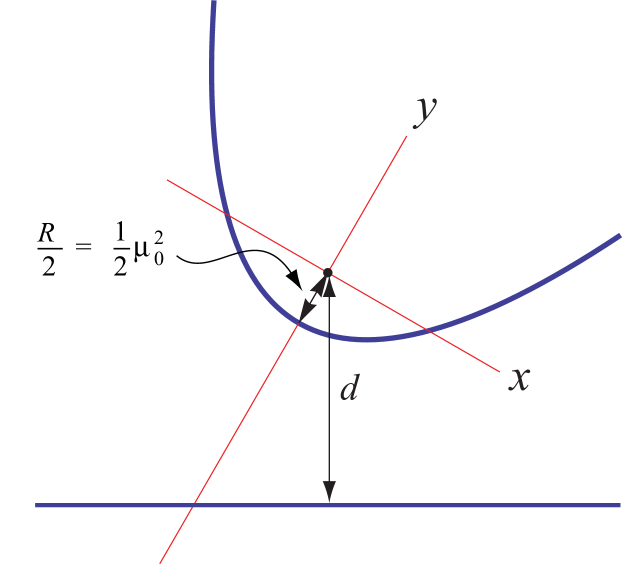
The surface of a parabolic cylinder in Cartesian coordinates is described by for all , as shown in Fig. 1, where is the radius of curvature at the tip. In parabolic cylinder coordinates MF , defined through , , , the surface is simply for . One advantage of the latter coordinate system is that the Helmholtz equation
| (1) |
which we consider for imaginary wavenumber , admits separable solutions. Since sending and returns us to the same point, we restrict our attention to while considering all values of . Then plays the role of the “radial” coordinate in scattering theory and we have regular and outgoing wave solutions
| (2) | |||||
| (3) |
where is the parabolic cylinder function, and and similarly for . Enforcing the reflection symmetry and for the regular solutions restricts the separation constant to integer values. The corresponding outgoing solutions do not obey this restriction and thus can only be used away from ; as is typical for outgoing solutions, they are irregular at . For imaginary wavenumber, the regular (outgoing) solutions grow (decay) exponentially in and both and are real. We can then express the free scalar Green’s function as MF
| (4) |
where () is the coordinate with the smaller (larger) value of . We will also use the Green’s function in coordinates appropriate to scattering from a plane perpendicular to the -axis,
| (5) | |||||
| (6) |
where . We can connect the parabolic and Cartesian Green’s functions using the expansion of a plane wave in regular parabolic solutions MF
| (7) |
where . This expression converges in regions where . A plane wave with can instead be expanded in terms of solutions with negative integer values of MF , and the Green’s function can also be expressed in terms of these functions analogously to Eq. (4). Restricting to is sufficient for our calculation, however, because we can already construct the Green’s functions from these solutions alone; in the formalism of Refs. spheres ; universal , all possible quantum fluctuations are captured through the Green’s function. Equating Eqs. (4) and (6) and then using (7), we obtain the expansion of the outgoing parabolic solution in plane waves,
| (8) |
which is valid for .
The regular and outgoing waves provide two independent solutions to the second-order differential equation. We take a linear combination of these solutions to obtain the scattering solution outside the parabolic cylinder. Fixing the coefficients by imposing Dirichlet boundary conditions at , we obtain
| (9) |
while for Neumann boundary conditions we have
| (10) |
These solutions to the Helmholtz equation can be used to compute the Casimir forces between a parabolic cylinder and other simple objects, for example an infinite plate, as depicted in Fig. 1. If both objects are perfect mirrors, translational symmetry along the -axis enables us to decompose the electromagnetic field into two scalar fields, with Dirichlet and Neumann boundary conditions respectively. Each scalar field can then be treated independently, with the sum of their contributions giving the full electromagnetic result. The quantization of each scalar field is achieved by integrating the exponentiated action over all configurations of the field GK . Constraining the fields to obey the boundary conditions on each surface leads to an alternative description involving fluctuating “charges” and on the surfaces spheres ; universal . Appropriate multipoles of these charges are
| (11) | |||||
The action can be decomposed in terms of these multipoles as , with
| (12) | |||||
Here corresponds to the action for the charges on the plane, with scattering amplitudes for Neumann and Dirichlet modes respectively. The corresponding action for charges on the parabolic cylinder can be related to its scattering amplitudes universal ; from Eqs. (9) and (10) we obtain
| (14) | |||||
| (15) |
The position and orientation of the parabolic cylinder relative to the plane enter only through the translation matrix , which appears in the interaction term . From Eq. (8), we obtain
| (16) |
where is the angle of inclination of the parabolic cylinder and is the distance from the focus of the parabola to the plane, as shown in Fig. 1.
Integrating over these charge fluctuations gives the Casimir energy per unit length as
Numerical computations are performed by truncating the determinant at index . For the numbers quoted below, we have computed for up to and then extrapolated the result for , and in the figures we have generally used . We note that the integrals over and can be expressed as a single integral in polar coordinates, and for the integral is symmetric and the translation matrix elements vanish for odd. Since the plane we are considering is a perfect mirror, is independent of and we can further simplify the calculation for using the integral
| (18) |
where is the Bateman -function Bateman , which is zero if is a negative even integer. Here is the confluent hypergeometric function of the second kind.
As a first demonstration, we report on the dependence of the energy on the separation for . At small separations () the PFA, given by
| (19) |
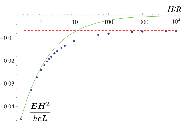
should be valid. The numerical results in Fig. 2 confirm this expectation with a ratio of actual to PFA energy of at (for ). We note that since the main contribution to PFA is from the proximal parts of the two surfaces, the PFA result in Eq. (19) also applies to a circular cylinder with the same radius .
A more interesting limit is obtained when , corresponding to a semi-infinite plate. Then the PFA result is zero, as are results based on perturbative approximation for the dilute limit Milton . The scattering amplitudes in Eq. (15) simplify and can be combined together as , where even corresponds to Dirichlet and odd corresponds to Neumann. Using this result, our expression for the energy for and simplifies to
| (20) | |||||
| (21) |
where is obtained by numerical integration. This geometry was studied using the world-line method for a scalar field with Dirichlet boundary conditions in Ref. Gies . The world-line approach requires a large-scale numerical computation, and it is not known how to extend this method to Neumann boundary conditions (or any case other than a scalar with Dirichlet boundary conditions). In our calculation, the Dirichlet component of the electromagnetic field makes a contribution to our result, in reasonable agreement with the value of in Ref. Gies .
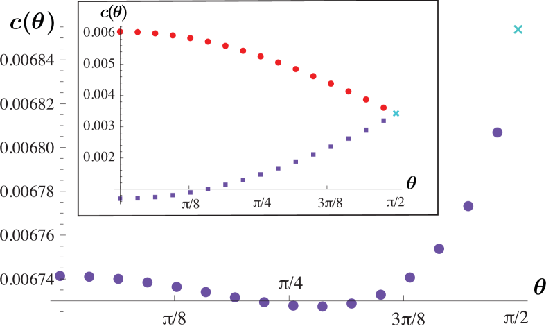
Reference Gies also considers a tilted semi-infinite plate, which corresponds to the limit of our formula for general . From dimensional analysis, the Casimir energy at again takes the now -dependent form
| (22) |
where for . Following Ref. Gies , we plot in Fig. 3. A particularly interesting limit is , when the two plates are parallel. In this case, the leading contribution to the Casimir energy should be proportional to the area of the half-plane according to the parallel plate formula, with , plus a subleading correction due to the edge. Multiplying by removes the divergence in as . As in Ref. Gies , we assume , although we cannot rule out the possibility of additional non-analytic forms, such as logarithmic or other singularities. With this assumption, we can estimate the edge correction from the data in Fig. 3. From the inset in Fig. 3, we estimate the Dirichlet and Neumann contributions to this result to be (in agreement with Gies within our error estimates) and respectively. Because higher partial waves become more important as , reflecting the divergence in in this limit, we have used larger values of for near .
It is straightforward to extend these results to nonzero temperature . We simply replace the integral by the sum over Matsubara frequencies , where the prime indicates that the mode is counted with a weight of universal . In the limit of infinite temperature, only the mode contributes and we obtain for the energy , with . The Dirichlet contribution to our result is , again in agreement with Gies .
Employing the scattering formalism, we can also calculate the Casimir energy for the case where another object whose scattering amplitudes are available, such as an ordinary cylinder or a second parabolic cylinder, is positioned outside the parabolic cylinder. Centering the other object at the origin and letting the parabolic cylinder open downward, with its focus displaced to , we obtain the necessary translation matrix elements by writing Eq. (8) for , where , , , and then expanding the plane wave on the right-hand side in the basis appropriate to the other object. Again we can allow the parabolic cylinder to tilt by replacing by in this expression. These results can be extended to multiple objects, as in Ref. JamalAlejandro . Another interesting possibility would be to apply the interior Casimir formalism of Ref. interior an object inside a parabolic cylinder, potentially extending the results of Ref. Ford ; Lombardo .
The reduction of the parabolic cylinder to a semi-infinite plate enables us to consider a variety of edge geometries. A thin metal disk perpendicular to a nearby metal surface would experience a Casimir force described by an extension of Eq. (20). Figure 2 shows that the PFA breaks down for a thin plate perpendicular to a plane; the PFA approximation to the energy vanishes as the thickness goes to zero, while the correct result instead has a different power law dependence on the separation. Based on the full result for perpendicular planes, however, we can formulate an “edge PFA” that yields the energy by integrating from Eq. (20) along the edge of the disk. Letting be the disk radius, in this approximation we have , which is valid if the thickness of the disk is small compared to its separation from the plane. (For comparison, note that the ordinary PFA for a metal sphere of radius and a plate is proportional to .)
A disk may be more experimentally tractable than a plane, since its edge does not need to be maintained parallel to the plate. One possibility would be a metal film, evaporated onto a substrate that either has low permittivity or can be etched away beneath the edge of the deposited film. Micromechanical torsion oscillators, which have already been used for Casimir experiments Decca07 , seem readily adaptable for testing Eq. (22). Because the overall strength of the Casimir effect is weaker for a disk than for a sphere, observing Casimir forces in this geometry will require greater sensitivities or shorter separation distances than the sphere-plane case. As the separation gets smaller, however, the dominant contributions arise from higher-frequency fluctuations, and deviations from the perfect conductor limit can become important. While the effects of finite conductivity could be captured by an extension of our method, the calculation becomes significantly more difficult in this case because the matrix of scattering amplitudes is no longer diagonal.
To estimate the range of important fluctuation frequencies, we consider and . In this case, the integrand in Eq. (20) is strongly peaked around . As a result, by including only values of up to , we still capture of the full result (and by going up to we include 99%). This truncation corresponds to a minimum fluctuation wavelength . For the perfect conductor approximation to hold, must be large compared to the metal’s plasma wavelength , so that these fluctuations are well described by assuming perfect reflectivity. We also need the thickness of the disk to be small enough compared to that the deviation from the proximity force calculation is evident (see Fig. 2), but large enough compared to the metal’s skin depth that the perfect conductor approximation is valid. For a typical metal film, and at the relevant wavelengths. For a disk of radius , the present experimental frontier of sensitivity corresponds to a separation distance , which then falls within the expected range of validity of our calculation according to these criteria. The force could also be enhanced by connecting several identical but well-separated disks. In that case, the same force could be measured at a larger separation distance, where our calculation is more accurate.
We thank U. Mohideen for helpful discussions. This work was supported by the National Science Foundation (NSF) through grants PHY05-55338 and PHY08-55426 (NG), DMR-08-03315 (SJR and MK), Defense Advanced Research Projects Agency (DARPA) contract No. S-000354 (SJR, MK, and TE), by the Deutsche Forschungsgemeinschaft (DFG) through grant EM70/3 (TE), and by the U. S. Department of Energy (DOE) under cooperative research agreement #DF-FC02-94ER40818 (RLJ).
References
- (1) H. B. G. Casimir, Proc. K. Ned. Akad. Wet. 51, 793 (1948).
- (2) S. K. Lamoreaux, Phys. Rev. Lett. 78, 5 (1997); U. Mohideen and A. Roy, Phys. Rev. Lett. 81, 4549 (1998); G. Bressi, G. Carugno, R. Onofrio, and G. Ruoso, Phys. Rev. Lett. 88, 041804 (2002); H. B. Chan, V. A. Aksyuk, R. N. Kleiman, D. J. Bishop, and F. Capasso, Science 291, 1941 (2001).
- (3) F. Capasso, J. N. Munday, D. Iannuzzi and H. B. Chan, IEEE J. Sel. Top. Quant. 13, 400 (2007).
- (4) M. T. Homer Reid, A. W. Rodriguez, J. White, and S. G. Johnson, Phys. Rev. Lett. 103, 040401 (2009).
- (5) T. Emig, N. Graham, R. L. Jaffe, and M. Kardar, Phys. Rev. Lett. 99, 170403 (2007); Phys. Rev. D 77, 025005 (2008).
- (6) S. J. Rahi, T. Emig, N. Graham, R. L. Jaffe and M. Kardar, Phys. Rev. D 80, 085021 (2009).
- (7) T. Emig, J. Stat. Mech. P04007 (2008).
- (8) S. J. Rahi, T. Emig, R. L. Jaffe, and M. Kardar, Phys. Rev. A 78, 012104 (2008).
- (9) P. Morse and H. Feshbach, Methods of Mathematical Physics (McGraw-Hill, 1953). See also E. H. Newman, IEEE Trans. on Ant. and Prop. 38, 541 (1990); D. Epstein, New York Univ. Inst. of Math. Sci., Div. of Electromagnetic Research, Rept. No. BR-19 (1956).
- (10) T. Emig, A. Hanke, R. Golestanian, and M. Kardar, Phys. Rev. Lett. 87, 260402 (2001).
- (11) H. Bateman, Trans. Amer. Math. Soc. 33, 817 (1931).
- (12) K. A. Milton, P. Parashar and J. Wagner, Phys. Rev. Lett. 101, 160402 (2008).
- (13) H. Gies and K. Klingmuller, Phys. Rev. Lett. 97, 220405 (2006); A. Weber and H. Gies, arXiv:0906.2313 [hep-th].
- (14) S. J. Rahi, A. W. Rodriguez, T. Emig, R. L. Jaffe, S. G. Johnson, and M. Kardar, Phys. Rev. A 77, 030101(R) (2008).
- (15) S. Zaheer, S. J. Rahi, T. Emig, and R. L. Jaffe, arXiv:0908.3270 [quant-ph].
- (16) L. H. Ford and N. F. Svaiter, Phys. Rev. A 62, 062105 (2000); Phys. Rev. A 66, 062106 (2002).
- (17) F. C. Lombardo, F. D. Mazzitelli, M. Vazquez and P. I. Villar, Phys. Rev. D 80, 065018 (2009).
- (18) R. S. Decca, D. López, E. Fischbach, G. L. Klimchitskaya, D. E. Krause, and V. M. Mostepanenko, Phys. Rev. D 75, 077101 (2007).