Tutorial on ABC rejection and ABC SMC for parameter estimation and model selection
In this tutorial we schematically illustrate four algorithms:
We suggest to read this tutorial from the beginning. We start with a detailed explanation of the ABC rejection algorithm, which later helps to understand ABC SMC as it is based on the same concepts. Also, both model selection algorithms are closely related to parameter estimation algorithms and it is therefore helpful to understand those first.
This tutorial forms a part of the supplementary material of the paper ”Simulation-based model selection for dynamical systems in systems and population biology, Bioinformatics, 26 (1), 104-110, 2010” (T. Toni, M. P. H. Stumpf).
ABC rejection
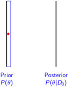
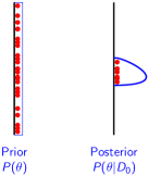
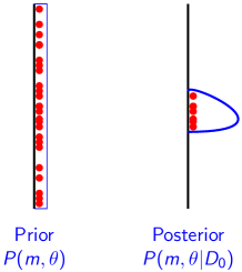
(a) We define a prior distribution and we would like to approximate the posterior distribution . We start by sampling a parameter from the prior distribution. We call this sampled parameter a particle.
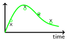
(b) We simulate a data set according to some simulation framework . In our examples we use different simulation frameworks. If we simulate a deterministic dynamical model, we add some noise at the time points of interest. If we simulate a stochastic dynamical model, we do not add any additional noise to the trajectories. We compare the simulated data set (circles) to the experimental data (crosses) using a distance function, , and tolerance ; if , we accept . The tolerance is the desired level of agreement between and .
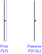
(c) The particle is accepted because and are sufficiently close.
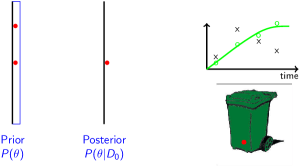
(d) We sample another parameter from the prior distribution and simulate a corresponding dataset . In this case and are very different and we reject the particle (we ”throw it away”).
(e) We repeat the whole procedure until N particles have been accepted. They represent a sample from , which approximates the posterior distribution. If is sufficiently small then the distribution will be a good approximation for the “true” posterior distribution, .
(f) Many particles were rejected in the procedure, for which we have spent a lot of computational effort for simulation. ABC rejection is therefore computationally inefficient. We can use ABC SMC to reduce the computational cost.
ABC SMC (Toni et al., 2009)
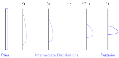
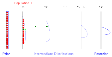
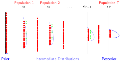
(a) As in ABC rejection, we define a prior distribution and we would like to approximate a posterior distribution . In ABC SMC we do this sequentially by constructing intermediate distributions, which converge to the posterior distribution. We define a tolerance schedule .
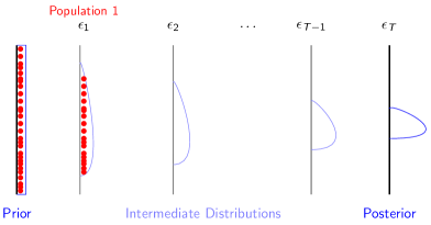
(b) We sample particles from a prior distribution until particles have been accepted (have reached the distance smaller than ). For all accepted particles we calculate weights (see [4] for formulas and derivation). We call the sample of all accepted particles ”Population 1”.
(c) We then sample a particle from population 1 and perturb it to obtain a perturbed particle , where K is a perturbation kernel (for example a Gaussian random walk). We then simulate a dataset and accept the particle if . We repeat this until we have accepted particles in population 2. We calculate weights for all accepted particles.
(d) We repeat the same procedure for the following populations, until we have accepted particles of the last population and calculated their weights. Population is a sample of particles that approximates the posterior distribution.
ABC SMC is computationally much more efficient than ABC rejection (see [4] for comparison).
ABC rejection for model selection
ABC SMC for model selection
![[Uncaptioned image]](/html/0910.4472/assets/x14.png)
![[Uncaptioned image]](/html/0910.4472/assets/x15.png)
![[Uncaptioned image]](/html/0910.4472/assets/x16.png)
![[Uncaptioned image]](/html/0910.4472/assets/x17.png)
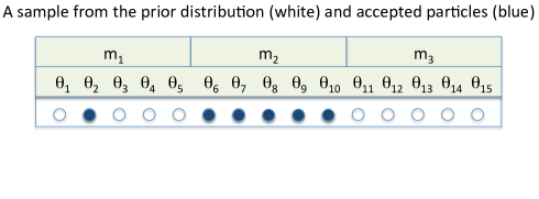
(a) Particles are sampled from the prior until particles have been accepted (in this example for illustration purposes, in practice should be larger), that is the distance is smaller than . The weights are calculated for all accepted particles and normalized.
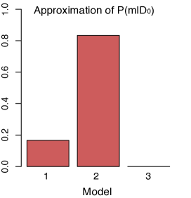
(b) To obtain the marginal probability of , we sum over all the weights corresponding to the model of interest: . The histogram of the marginal population is presented.
(c) This figure shows how we propose and accept a particle of population , . We sample a model from population with probability . For example, we might have sampled . We then perturb the model using a model perturbation kernel to obtain , for example . After we have obtained the model , we sample a parameter belonging to model from population and perturb it to obtain . We simulate a dataset for a particle and accept () or reject the particle. If a particle is accepted, we calculate its weight .
(d) When particles of population have been accepted, we normalize the weights and marginalize them in order to obtain the marginal intermediate population of the model . We continue until population , which is the approximation of the joint posterior distribution . The quantities of interest are the intermediate and the last marginal population of the model. In this example there are three populations, .
References
- [1] Beaumont MA, Zhang W and Balding DJ. Approximate Bayesian computation in population genetics. Genetics, 162(4):2025–2035, 2002.
- [2] Marjoram P, Molitor J, Plagnol V and Tavare S. Markov chain Monte Carlo without likelihoods. Proc Natl Acad Sci USA, 100(26):15324–8, 2003.
- [3] Sisson SA, Fan Y and Tanaka MM. Sequential Monte Carlo without likelihoods. Proc Natl Acad Sci USA, 104(6):1760–5, 2007.
- [4] Toni T, Welch D, Strelkowa N, Ipsen A and Stumpf MPH. Approximate Bayesian computation scheme for parameter inference and model selection in dynamical systems. J. R. Soc. Interface, 6:187–202, 2009.
- [5] Beaumont MA, Cornuet JM, Marin JM and Robert CP. Adaptive approximate Bayesian computation. Biometrika, 96(4):983–990, 2009.
- [6] Grelaud A, Robert CP, Marin JM, Rodolphe F and Taly JF. ABC likelihood-free methods for model choice in Gibbs random fields. Bayesian Analysis, 4(2):317–336, 2009.
- [7] Toni T and Stumpf MPH. Simulation-based model selection for dynamical systems in systems and population biology. Bioinformatics, 26(1):104–10, 2010.