Theory of the time-resolved Kerr rotation on trapped holes
Abstract
We formulate a model of the time-resolved Kerr rotation experiment on an ensemble of independent holes in a semiconductor nanostructure (e.g., confined in a quantum dot or trapped in a quantum well) in a tilted magnetic field. We use a generic Markovian description of the hole and trion dephasing and focus on the interpretation of the time-resolved signal in terms of the microscopic evolution of the spin polarization. We show that the signal in an off-plane field contains components that reveal both the spin relaxation rate and the spin coherence dephasing rate. We derive analytical formulas for the hole spin polarization, which may be used to extract the two relevant rates by fitting to the measurement data.
pacs:
78.67.De, 78.67.Hc, 78.47.jcI Introduction
In recent years, considerable experimental progress has been achieved in the optical control and readout of spin states of electrons and holes in semiconductor nanostructures shabaev03 ; dutt05 ; greilich06c ; kennedy06 ; atature07 ; greilich07 ; press08 ; gerardot08 . Extended life times of spin states in quantum dots (QDs) paillard01 and quantum wells (QWs) kikkawa97 seem very promising for applications in spintronics, e.g. in the form of spin memory kikkawa97 ; kroutvar04 , or in semiconductor spin-based quantum computing loss98 ; hawrylak05 . Particular expectations are related to hole spins, since the reduced hyperfine interaction in this case makes the hole spin decoherence even slower heiss07 ; brunner09 .
In order to design feasible spin-based devices, one obviously has to understand the properties of spins in confined semiconductor systems. The most essential parameters that must be known in order to predict the evolution of a spin in a real structure are the Landé -tensor, which defines the unitary evolution of a spin in a magnetic field, and the relaxation (dephasing) times, accounting for the impact of the environment. As the Zeeman shifts can be rather small and, therefore, hard to resolve spectrally, many experiments rely on time-resolved methods bar-ad91 ; damen91 ; marie99 ; palinginis04 . Among those, time-resolved Faraday tribollet03 ; meier07 ; yugova07 ; atature07 or Kerr malinowski00 ; zhukov07 ; syperek07 ; zhukov09 ; kugler09 rotation measurements have proven to be very useful. In these experiments, one studies the rotation of the polarization plane of transmitted or reflected radiation (probe pulse) due to spin polarization excited by a circularly polarized pump pulse. In this way, the decay of spin polarization and the spin precession around the quantization axis can be observed as a function of delay time between the pulses.
The theoretical challenge in the description of confined hole spin properties is essentially three-fold. First, one has to model the nanostructure in order to find the effective -factor for holes in a two- or zero-dimensional confinement. This is usually done using methods marie99 ; zhao94a ; zhao94b and the results are in reasonable agreement with measurements. Second, one needs to describe the spin dephasing and relaxation processes. Phonon-mediated processes are often invoked for QDs woods04 ; bulaev05a , although other channels are also taken into account sanjose06 . In QWs, phonons are expected to dominate for trapped holes, while scattering due to compositional disorder is invoked for delocalized ones ikonic01 . Another reason for dephasing may be system inhomogeneity, in particular -factor fluctuations semenov02 .
In the present paper, we deal with the third aspect of the problem, namely, the microscopic origin of the measured signal and, more importantly, the relation between the magnetic (spin) orientation, which is supposed to be studied, and the optical field, which is experimentally accessible. We analyze also in what way the optical response (in particular, Kerr rotation) of the system depends on the parameters characterizing the system evolution. In the case of a time-resolved experiment with pulsed excitation, the physical interpretation of the detected optical response becomes non-trivial and constitutes a subject of study by itself zhang09 ; yugova09 . This kind of theoretical discussion has been presented for excitons in a QW ostreich95 and, on a phenomenological level, for an n-doped QW system zhukov07 . Very recently, a complete analysis of the Kerr and Faraday response for ensembles of n-doped QDs in an in-plane magnetic field was presented yugova09 . Here, we focus on trapped hole states in QWs and on holes confined in QDs. We discuss the microscopic origin of the time-resolved Kerr rotation (TRKR) signal in a pump-probe experiment on a p-doped sample in tilted magnetic field. We perform a complete analysis in the density matrix formalism and describe hole spin dephasing on a general level, assuming only its Markovian character. Our description is applicable to various decoherence processes that have a well-defined Markov limit wchich is applicable under given conditions. Examples of such processes include phonon-assisted transitions or Coulomb scattering. We discuss how the “longitudinal” and “transverse” dephasing rates (defined with respect to the tilted quantization axis) manifest themselves in the detected TRKR signal.
As a result of our study, we point out that the optical signal follows the spin polarization in the limit of strong dephasing of optical coherences. The same holds true in the case of long-lived optical coherences if the phase relation between the pulses can be considered random or, for an extended system, if the experimental geometry assures that the coherent part of the signal is emitted in a different direction. We show that the dephasing of the hole spin precession beats is governed by two rates involving a combination of the two relaxation rates. In a homogeneous system, this may allow one to extract both rates from a single experiment. In addition, we study the effect of inhomogeneity of -factors on the observed TRKR signal.
The paper is organized as follows. In Sec. II, we describe the system and the experiment to be modelled. The next Sec. III contains the microscopic derivation of the optical TRKR signal. In Sec. IV, we study the spin dynamics using a general model of Markovian decoherence, including also inhomogeneous dephasing. The relation between the optical signal and the spin polarization is discussed in Sec. V. In Sec. VI, we present the results of our simulations and discuss the dependence of the TRKR signal on the off-plane tilt angle of the magnetic field and on the relative strength of different contributions to dephasing (longitudinal, transverse, inhomogeneous). These results are discussed in the next Sec. VII. The appendix contains the derivation of the general Lindblad equation describing Markovian decoherence in the hole-trion spin system.
II The system
We consider the optical response of a system composed of trapped (localized) holes which may be considered independent (non-interacting). This situation may correspond to a p-doped quantum well in which holes are localized by some kind of trapping potentials, e.g., interface fluctuations or nearby defects. The theory applies also to ensembles of quantum dots in a remotely p-doped structure. In thermal equilibrium, each trapping center is assumed to accommodate one hole. The area density of such trapped holes is . Only heavy hole states are considered, since the heavy-light hole splitting is usually large in confined systems. The fundamental optical transition at each trapping center consists in an excitation of an electron-hole pair which, together with the resident hole, forms a bound trion. It is assumed that the temperature is low and the driving pulses are spectrally narrow enough to restrict the description to the lowest hole and trion states. The system is placed in a magnetic field oriented at an angle with respect to the growth axis. The quantum well or layer of QDs is covered by a capping layer of thickness .
A single trapped hole-trion system is described by the Hamiltonian
| (1) |
where is the Bohr magneton, is the hole Landé tensor, is the Landé factor of the trion (i.e., essentially, of the electron), which we assume isotropic, and are the vectors of Pauli matrices corresponding to the hole and trion spin, respectively (the hole is treated as a pseudo-spin-1/2 system). Here and in the following, we describe the system in a reference frame rotating with the zero-field hole-trion transition frequency .
The spin states of each hole or trion can be described in terms of the “spin up” and “spin-down” states, that is, the basis states with definite projections on the growth axis (normal to the QW or to the plane of QDs), (for a hole) and (for a trion). For the magnetically isotropic trion, we define the two Zeeman eigenstates
In the case of the hole, the quantization axis does not necessarily coincide with the field orientation. The hole spin eigenstates can be written as
where is a certain angle depending on the structure of the hole Landé tensor. In our simulations, the latter will be assumed isotropic in the structure plane, so that
| (2) |
where and are the in-plane and axial components of . The Zeeman energy splitting for the hole is then , Note, however, that the actual structure of the Landé tensor enters the theory only via the the angle and the Zeeman energy which can easily be found also for structures with a more complicated form of the Landé tensor kusraev99 .
A laser tuned to the trion line excites the system by two pulses (pump-probe configuration). The pulses propagate nearly perpendicular to the structure plane (a small deviation of the probe beam from the perpendicular axis is needed to separate the contributions to the third order response, as discussed in Sec. V). The first pulse arrives at and is circularly polarized (). The second, linearly () polarized one arrives at . The amplitudes of the electric field in the two pulses (outside the semiconductor) are , . The electric field couples to the interband transitions via a dipole moment . The pulse shape is described by a function , which is of the order of unity. The pulse length will be denoted by . The reflection amplitude at the semiconductor-vacuum interface is , where is the refractive index of the capping layer. The relevant Hamiltonian in the rotating wave approximation is then
| (3) | |||||
where are the effective amplitudes of the two pulses inside the material. For the pulse shapes we will assume Gaussians, .
In addition to the evolution governed by the Hamiltonian , the system undergoes dissipative dynamics due to the interaction with its environment. As long as this decoherence can be described in the Markov limit (which is reasonable in view of the relatively long time scales involved), its effect on the hole spin can be described by the universal Lindblad superoperator (see Appendix A). In this limit, the open system evolution is described by three dephasing rates: describe the longitudinal decoherence, that is, spin relaxation between the Zeeman eigenstates for a given field orientation, while accounts for additional pure dephasing processes. The two spin-flip rates are related by
which guarantees the detailed balance condition at equilibrium. Here is the transition rate for a “down-flip” (from the upper to the lower Zeeman state), and is the rate for an “up-flip”. Note that, apart from this relation, in a specific model of hole-reservoir interaction, the rates will depend on the Zeeman splitting and temperature via the spectral density of the relevant reservoir [see Eq. (28)]. However, in our general discussion, we treat one of them (or their sum) as a parameter of the model.
The Lindblad dissipator describing the hole decoherence has the form
| (4) | |||||
where
An analogous dissipator describes the spin dephasing of the trion. However, since the trion spin coherence time is much longer than its lifetime, the decay of spin coherence will be governed by the latter and the trion spin dephasing can be neglected. Note that the spin dephasing in the Markov limit is necessarily described in the eigen basis defined by the field orientation, which differs from the “spin-up” and “spin-down” basis defined by the structure symmetry and by the optical selection rules.
The last part of the model is the radiative decay of the trion, which is accounted for by the Lindblad superoperator
| (5) | |||||
where is the radiative decay rate, is the additional pure dephasing rate, and the transition operators are
Note that the distinction between the trion recombination and pure dephasing is essential here not only because of the presence of various pure dephasing mechanisms in real systems krummheuer02 ; borri05 ; muljarov04 ; machnikowski06e but, much more importantly, because of the different effect these processes have on the spin-dependent optical response: both of them contribute to the decay of the optical polarization but pure dephasing, contrary to recombination, does not affect the trion spin occupations. In an ensemble of emitters, the dephasing of trion coherences can be in fact dominated by inhomogeneous effects (distribution of the trion transition frequencies). This would result in a different form of the coherence decay. However, from the point of view of the present study, this difference is of minor importance and only the characteristic time of the coherence decay is essential. Therefore, we simplify the discussion by neglecting this kind of inhomogeneity and using only the pure dephasing rate to characterize the optical dephasing.
III The TRKR response
In this Section, we define the measured TRKR signal and clarify its relation to the microscopic variables (elements of the density matrix) defining the state of the carriers in a nanostructure at the moment when the probe pulse arrives. We show how the phenomenology of Kerr rotation emerges in the homodyne detection process from the interference of the macroscopic optical field reflected from the system surface with the radiation due to the interband optical polarization in the nanostructure. Finally, we relate the latter to the spin polarization.
The experimentally measured effect is a rotation of the polarization plane of the probe beam reflected from the sample. The total field is projected onto the two axes , oriented at with respect to the polarization of the probe beam. The rotation of the polarization axis is given by the difference of intensity between the corresponding two components of the field yugova09 ; zhukov07 ,
| (6) |
where and denote the (complex) amplitudes of the circularly right- and left- polarized components of the total field and denotes time averaging over the period of the electromagnetic field.
On the microscopic level, the observed reflected field is a sum of the beam reflected at the surface of the capping layer (this process will be treated on the usual, macroscopic level) and the field emitted by the nanostructure. Thus, the two circular polarization components of the total field incident at the detector are
| (7) |
where is the field reflected from the surface of the capping layer and is the field emitted by the carries trapped in the nanostructures. For pulsed excitation, slow evolution of the field amplitudes has to be taken into account. The field reflected at the surface simply follows the pulse envelope and the amplitudes of its and components at the sample surface are both equal to
| (8) |
The optical signal emitted from the structure originates from the interband polarization. If denotes the density matrix representing the system state then each trapped hole-trion superposition contributes a component of the dipole moment and a component . This results in the polarization current
(and analogous for ) and the amplitudes of the corresponding two components of the radiation emitted from the structure (at the sample surface) are
| (9) |
where is the phase shift (with respect to the field ) due to propagation through the capping layer.
Note that if the two components have equal phases (as is indeed the case, see below) then the radiation emitted from the nanostructure is, in general, elliptical but its polarization axis is not rotated. Moreover, the intensity of this signal is weak. What one really measures in the homodyne detection scheme is, however, the signal coherently superposed on the much stronger field reflected from the surface of the sample. Substituting Eqs. (8) and (9) into Eq. (7) and then into Eq. (6) and retaining only terms of the first order in the nanostructure response one finds the TRKR signal
| (10) | |||||
In the above discussion, we have assumed that all the hole-trion systems evolve under the same conditions. The effect of inhomogeneity will be treated in Sec. IV.2. Eq. (10) describes the measured signal in terms of the quantum state of a nanostructure. This equation can be used to find the system response without any further simplifying assumptions based on a numerical simulation of the open system evolution.
The next step is to derive the relation between the elements of the density matrix and the spin polarization before the arrival of the probe pulse. This relation can be expressed in an analytical form yugova09 under the assumption that the probe pulse is much shorter than any relevant time scale of the system dynamics (consistent with the idea that it is supposed to probe the instantaneous state of the system). One has to assume also that the dephasing times of interband coherences are longer than the pulse duration.
In order to relate the Kerr response to the density matrix formalism we note that the system state , which gives rise to the measured polarization, is prepared by the probe pulse from the state just before this pulse, , where denotes the time instant just before the arrival of the probe pulse. Under conditions stated above, we can completely neglect the system evolution during the pulse. Then, the system density matrix is transformed according to , with the unitary operator
where
With this time evolution operator one finds for the interband matrix elements (for )
| (11) | |||||
Let us first assume that the delay time between the pump and the probe pulse is much longer than the interband dephasing time. (We will come back to the case when this is not fulfilled in Sec. V). In this case, the interband matrix elements at time are negligible and we only have the contributions proportional to , i.e., the terms involving the occupation differences between trion and hole states. Substituting this into Eq. (10) and using the expression (8) for the reflected field we find for the TRKR signal
| (12) | |||||
where
| (13a) | |||||
| (13b) | |||||
are trion and hole spin polarizations, respectively.
We neglect here the delay between the field envelopes due to propagation through the capping layer, which is of the order of 1 fs, that is, much shorter than the picosecond pulse duration. The signal described by Eq. (12) is proportional to the difference of hole and trion spin polarizations just before the probe pulse. In this way, the TRKR measurement gives access to the evolution of the spin polarizations in the system.
For a pulsed excitation, depends on time. We define the time-integrated (TI) TRKR signal as
| (14) |
This quantity is a function of the time delay between the pump and probe pulses. Since the homodyne response is proportional to the envelope of the probe pulse, the integration in the above equation is done over the duration of the probe pulse.
We note that
where
is the area of the probe pulse. Hence, the integrated detection signal is (see also Ref. yugova09, )
| (15) |
In the weak pulse limit, the spin polarizations are proportional to the intensity of the pump pulse, hence the signal is also proportional to this intensity. Moreover, it follows directly from Eq. (15) that in this limit the response is also proportional to the intensity of the probe pulse.
The quantity sets the natural energy scale for the emitted radiation and is equal to the energy the system would emit per unit area if each hole-trion system generated one photon. Thus, , which is the quantity to be plotted based on the results of simulations in Secs. V and VI, corresponds to the average number of photons per one hole-trion emitter and one repetition of the experiment.
IV Hole and trion spin decoherence
In this section we present a detailed analysis of the spin dynamics based on an analytical solution of the equation of motion for the density matrix in an idealized situation of coherent optical driving and fast dephasing of optical coherences. The validity of these assumptions and the relation between the quantities calculated here and the actual signal are discussed in Sec. V. We begin with a discussion of dephasing of a single system. Then we study the effect of inhomogeneity of -factors across the ensemble.
IV.1 Homogeneous dephasing
The set of dynamical variables describing the evolution of the system consists of the trion and hole populations
the trion and hole spin polarizations defined in Eqs. (13a) and (13b), as well as trion and hole spin coherences,
Initially, all trion variables are zero. The spin of the trapped hole is in the thermal equilibrium state, which, in the basis of the hole spin eigenstates, is characterized by a spin polarization
where is the density matrix for the system state at equilibrium. This corresponds to the following initial values for the dynamical variables of the holes:
In the present discussion, we assume that the pulse durations are much shorter than any characteristic time scale of the spin dynamics and their action may be approximately treated as instantaneous. This means that the excitation is coherent (the case of dephasing times comparable with pulse durations is discussed in Sec. V). We assume also that it is resonant (effects of detuning for the case of -doped structures and exact Voigt geometry have been studied in Ref. yugova09, ). Then, the effect of the pump pulse is to perform the rotation , where
and
is the pulse area. The pulse generates the trion population and depletes the hole population accordingly,
generates the hole and trion polarization,
and reduces the hole spin coherence which exists at thermal equilibrium in a tilted magnetic field
The other dynamical variables remain zero.
The subsequent dynamics of the system is generated by the Zeeman Hamiltonian and by the dissipators and ,
| (16) |
For the occupation, this yields a single decay equation with the obvious solution
When the trion spin dephasing is neglected the trion variables evolve according to a closed set of three equations,
where is the trion Larmor frequency. The solution for the trion spin polarization is easily found to be
| (17) |
For the hole variables, the equation of motion (16) leads to the system of equations with and acting as source terms,
where , , and
(the equilibrium values are subtracted). By the Laplace transform technique, one finds the solution for the hole spin polarization in the form
| (18) |
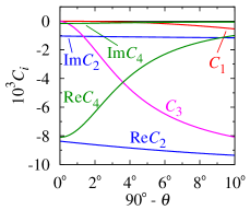
The exponents can be found exactly in a simple form, while the expressions for the amplitudes are rather lengthy, therefore we use the fact that the hole dephasing rates are much smaller than all the other rates and frequencies and give the formulas for in the leading order, that is, neglecting terms . The result is
The values of the amplitudes as a function of the orientation of the magnetic field for the parameters assumed in this paper (Tab. 1) are plotted in Fig. 1.
| Electron g factor | |
|---|---|
| Hole g factor | |
| – axial | |
| – in plane | |
| Trion recombination time | ps |
| Refractive index | |
| Pulse duration (pump & probe) | ps |
| Pulse amplitude | |
| – pump | meV |
| – probe | meV |
| Temperature | K |
| Magnetic field | T |
According to Eqs. (17) and (18), there are three kinds of contributions to the total spin polarization . The constant one, , corresponds to the equilibrium spin polarization. Exponentially decaying contributions, given by the first term in Eq. (17) and by the 1st and 3rd term in Eq. (18), originate from the decay of the spin population with respect to the respective quantization axes. Since we assumed that the trion spin lifetime is limited by the recombination time, the trion spin population decays with the recombination rate . The hole population decays with the spin relaxation rate . Since only spin polarization along the growth axis is relevant in the optical measurement, these contributions vanish when the spin quantization axis is perpendicular to the structure symmetry axis, that is, and for the hole and trion contributions, respectively. It should be noted that due to the strong anisotropy of the hole factor, the out-of-plane component of the hole spin is large already in a slightly tilted magnetic field. Therefore, the occupations of the Zeeman levels and their thermalization affect the optical response already in slightly tilted fields. The second term in Eq. (17) and the 2nd and 4th terms in Eq. (18) reflect the spin precession around the quantization axis. This precession affects the optically detected spin polarization only if the quantization axis is tilted with respect to the structure axis, that is, and .
IV.2 Inhomogeneous effects
If the measured signal originates form an ensemble of emitters, it becomes dephased due to variation of system parameters across the ensemble. In our case, non-uniformity of -factors makes the individual spins precess with various rates, which destroys the overall spin polarization.
We assume that the number of systems in the ensemble is sufficient to describe the distribution of -factors by a continuous distribution function. We neglect possible variation of the quantization axis. It is convenient to describe the inhomogeneity in terms of the trion and hole precession frequencies and , for which we assume Gaussian distributions
| (19) |
where , now become the central frequencies of the corresponding distributions. We assume that , so that a variation of the amplitudes in Eq. (18) can be neglected. Then, upon averaging with the distribution functions (19), the trion and hole spin polarizations [Eqs. (17) and (18)] become
| (20) | |||||
| (21) |
where the amplitudes are the same as in Eq. (18), for , , and . As usual, the exponential decay of a single system is replaced by a Gaussian one if the dispersion of frequencies is larger than the homogeneous dephasing rates.
V Spin polarization and TRKR response
The discussion presented in the previous sections was based on some simplifying assumptions. On the one hand, in our discussion of the TRKR response in Sec. III, we concentrated on delay times longer than the interband dephasing time. Therefore we did not discuss the contributions to the interband polarization resulting from the interband coherences created by the pump pulse. In quantum wells, such interband coherences vanish very quickly but in self-assembled quantum dots their lifetime may be limited only by the recombination time, which is of the order of a nanosecond langbein04 ; bayer02 . On the other hand, the derivation of the analytical formulas in Sec. IV, as well as of the relation between the spin polarization and the TRKR signal, is based on the assumption of coherent excitation. This, in turn, requires the coherence time to be long enough and the coherence assumption breaks if dephasing of the optical coherences is fast. In this section, we will deal with these issues.
In order to model the full optical response of the system we will numerically solve the evolution equation
| (22) |
calculate the optical signal according to Eq. (10), and integrate the result according to Eq. (14). Some of the parameters will be kept constant for all the results presented in this paper. The values of these fixed parameters (roughly correspopnding to an AlGaAs QW system similar to that studied in Ref. syperek07, ) are collected in Tab. 1. The trion Larmor frequency is ps-1. The pulse amplitudes chosen here correspond to the pulse areas and for the pump and probe pulse, respectively. These values assure that the optical excitation is well in the linear regime, so that varying the pulse areas leads only to uniform rescaling of the signal intensity proportionally to the pulse intensities, that is, to and .
First, we will discuss the additional contributions in the case of delay times shorter or of the same order as the interband dephasing time. In this case, also the interband terms at time in Eq. (11) contribute to the total interband matrix elements at time and thus to the emitted radiation. However, we notice that the phase of the second pulse enters differently in the three terms. Keeping in mind that the interband coherences created by the first pulse carry a phase factor (in the case of ) and (in the case of ), the total phases are for the first term, for the second term, and for the third term. Hence, only the second term holds a fixed phase relation with the reflected beam and can produce a non-vanishing homodyne signal if the relative phase between the pulses is random. Moreover, the two exciting laser pulses are usually applied to the sample at slightly different directions and . Then, for an extended system (ensemble of emitters), also the emitted radiation originating from the three contributions has different directions. The first one is emitted in the direction of the reflected pump pulse, the second one in the direction of the reflected probe pulse and the third one in the background-free reflected four-wave mixing direction . Thus we find that the interband coherences resulting from the pump pulse excitation indeed give rise to emitted signals, but they do not contribute to the TRKR signal [Eq. (10)]. The only exception would be the case of temporally overlapping pump and probe pulses, where the actions of pump and probe pulses cannot be treated separately, and the case of perfectly aligned, phase-locked pulses where the interference between the interband coherence from the first pulse and the second pulse gives rise to strong coherent control oscillations. Both cases, however, are not relevant for the purpose of this paper.
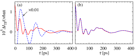
The numerical solution for the system evolution according to Eq. (22) does not involve any simplifying assumptions, apart from the resonant excitation condition. However, in this model, the geometrical relations between various directions in which the signals are emitted are not taken into account. Moreover, in a single simulation run, the relative phase between the pulses is fixed. Therefore, the calculated optical response contains both the TRKR signal and the coherent components. A comparison of the simulated signal to the spin polarization in this case, shown in Fig. 2(a), reveals that the former not only differs by orders of magnitude but also is uncorrelated to the latter. This is the case even for delay times a few times longer than the trion relaxation time since the coherent contribution belongs to a lower order of the optical response and is many orders of magnitude stronger in the weak excitation limit. The coherent artefacts can be eliminated from the simulation result by simply averaging the results obtained with opposite signs of the probe amplitude. If this is done, the simulated signal agrees with the analytical formulas, as expected [see Fig. 2(b)]. This confirms that the approximations made in the analytical solution do not noticeably affect the result.
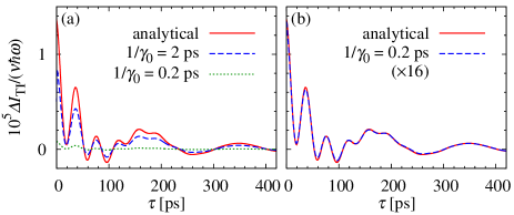
In the opposite case of strong interband dephasing, the analytical formulas are no longer valid. In Fig. 3(a) we compare the analytical result (red solid line) with the simulated signal for two values of the dephasing rate which describes additional pure dephasing of the optical coherence (beyond that associated with the radiative decay the rate of which, is fixed throughout the paper). As the dephasing time becomes comparable with the pulse duration, the signal is quenched due to the reduced efficiency of optical pumping and probing. We note, however, that this quenching is uniform, that is, it does not modify the shape of the pulse. This is clear from Fig. 3(b), where the simulated response for ps-1 has been multiplied by a factor of 16. Upon this rescaling, the simulated signal matches the analytically calculated one almost exactly.
Thus, we have established the relation between the evolution of spin polarization in the system and the form of the TRKR response. It turns out that both the simulated (or measured) signal and the analytical formula can yield consistent, correct information on the spin evolution. One has to eliminate the coherent polarization contributions from the calculated optical response in the slow dephasing case and the analytical formulas uniformly overestimate the signal in the case of fast optical dephasing.
VI Results
In this Section, we discuss the evolution of the spin polarization, based on the analytical solution to the equations of motion derived in Sec. IV. In all the simulations presented below, we set (hence, the term “pure dephasing” will always refer to the pure dephasing of spin states, described by the parameter ).
In Fig. 4(a), we show the evolution of the spin polarization for a certain set of parameters. The signal appears to be dominated by two oscillating components. As discussed in Sec. IV.1, the short-period one corresponds to the trion precession with the frequency . This contribution is damped with the rate due to the finite trion life time. The other oscillating contribution originates from the hole precession and is damped with the total hole spin dephasing rate , reflecting the decay of the hole spin coherence (transverse dephasing). Two other contributions, which are less evident in the plot, have a non-oscillating character and reflect the spin relaxation leading to thermalization between the Zeeman eigenstates (longitudinal decoherence). The presence of these parts of the signal becomes easily visible in the form of a central line in the Fourier transform of the TRKR response, shown in Fig. 4(b). We plot here also the individual contributions following from Eqs. (17) and (18).
The two most interesting aspects of the TRKR response are the dependence of the signal on the tilt angle between the magnetic field and structure plane and the effect of various dephasing types (spin relaxation, pure dephasing, inhomogeneous dephasing). In the following subsections, we start our analysis with the angle dependence and later proceed to the role of various dephasing contributions.
VI.1 Tilt angle dependence
Due to the strong anisotropy of the hole factor, the TRKR signal shows a very strong dependence on the angle at which the magnetic field is tilted off the system plane. The quantization axis of the hole spin is far from the plane even for small tilting angles. Therefore, the form of the signal changes strongly when is varied in the range of a few degrees from the in-plane orientation.
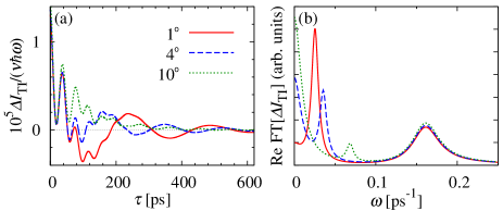
In Fig. 5(a) we show the TI-TRKR response for three different tilt angles between the magnetic field and the structure plane. In these calculations, we keep the same value of for all angles even though the Zeeman splitting changes, which is to some extent artificial. A correct dependence would follow from the detailed modeling of a specific decoherence channel, which is beyond the scope of the present general description. In all the cases shown in Fig. 5(a), one can clearly see a similar contribution from the trion Larmor precession. However, the hole contributions are different. The amplitude of the oscillations decreases as the field is tilted more off the plane. At , the hole contribution is dominated by a monotonous decay superposed on the trion oscillations. The reason for this is clear: For the tilt, the hole precesses around an almost in-plane quantization axis (oriented at about off-plane). Such a precession leads to a strong variation of the perpendicular component of the spin, while the thermalization of the spin occupations is associated mostly with the optically irrelevant decay of the in-plane component. On the contrary, according to Eq. (2), at the hole spin quantization axis is close to perpendicular (). The precession then takes place mostly in the plane, while the spin population decay affects the perpendicular spin polarization and is visible in the experiment.
This qualitative difference in the system evolution is visible even more clearly in Fig. 5(b), where we plot the real part of the Fourier transform of the TI-TRKR signals shown in Fig. 5(a). Three characteristic features are visible in this spectrum. Starting from the right, the broad one at ps-1 corresponds to the trion precession. The orientation of the magnetic field does not affect the position of this feature because the trion (electron) factor is isotropic. Moreover, for the narrow range of tilt angles considered here, the effect on the amplitude of the trion oscillations is very small. Therefore, this feature is almost insensitive to the orientation of the field in the considered range. The second feature moves from ps-1 at to ps-1 at and looses its amplitude. It corresponds to the hole precession. The frequency shift is obviously due to the growing contribution of the large axial component of the hole factor as the field is tilted off the plane. The decrease in amplitude corresponds to the fast reorientation of the hole spin quantization axis, which leads to reduced contribution of the hole precession to the optical signal. The third feature is the central line, corresponding to the exponential decay of the hole spin population. As the magnetic field is oriented more off-plane, the contribution of this process to the spin polarization grows and this feature becomes stronger.
VI.2 Dephasing
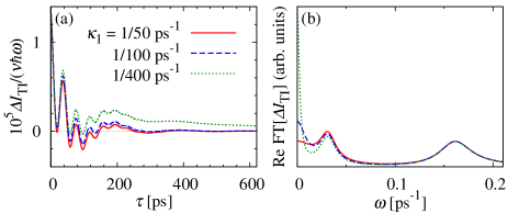
Another interesting feature observed in the simulation is a different dependence of the decay time of two hole-related components on the two hole decoherence rates and . This is visible in Fig. 6, where we fix the precession damping rate and change the relative contributions from the spin relaxation () and the additional pure dephasing (). In the time-resolved picture [Fig. 6(a)], the differences are not particularly characteristic, except for the long exponential tail which develops as the spin relaxation becomes very slow. Much more pronounced differences can be noticed in the Fourier transform [Fig. 6(b)]. As the parameter modification affects only the hole dynamics, the trion feature remains unchanged. Moreover, since we fixed the total dephasing time of the hole precession, the feature at the hole Larmor frequency, , changes very little (only due to the change in the tails of the neighboring zero-frequency feature). On the contrary, the central line changes very strongly. As the lifetime of the spin population becomes longer, this line gets narrower, with the line area remaining constant. It seems, therefore, that the spectral components of the TRKR signal in a tilted magnetic field carry useful information on the relative strength of different contributions to spin dephasing.
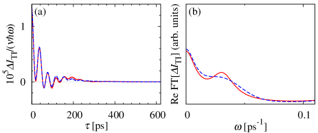
Another source of damping of the observed spin precession oscillations in the case of an ensemble measurement is the inhomogeneity of Larmor frequencies due to a variation of factors of the individual emitters in the ensemble. Obviously, only the precession-related contributions are sensitive to the inhomogeneity effects. Indeed, as follows from Eqs. (20) and (21) inhomogeneity affects the oscillating contributions, while the exponentially decaying ones remain unaffected. Since the main concern in the present work is the hole spin evolution, we will restrict the discussion to the case of . In Fig. 7, we show the evolution of the TRKR signal and the corresponding spectrum for a fixed value of the hole spin relaxation rate with the dephasing contribution dominated by the homogeneous pure dephasing (red solid lines) and by factor inhomogeneity (blue dashed lines). The parameters and are chosen such that the full width at half maximum of the damping envelope (in the time domain) is the same in the two cases. Again, there is only a minor change in the time-resolved signal [Fig. 7(a)]. However, the shape of the spectral feature corresponding to the hole spin precession changes from Lorentzian to Gaussian. This change may be characteristic enough to discriminate the homogeneous vs. inhomogeneous dephasing in a real measurement data.
VII Discussion and conclusion
We have developed a complete theory of the time-resolved Kerr rotation experiment for a system of trapped holes in tilted magnetic fields. The theory is applicable to quantum dots or weak trapping centers in quantum wells. In our approach, we adopted a general description of hole spin relaxation and dephasing in the Markov limit, based on the Lindblad equation for the open system dynamics. Spin dephasing is a rather slow process so that the Markov approximation should work well for this problem and our approach can be expected to cover a wide range of physical effects in a way which is independent of the exact microscopic mechanisms. One should note, however, that there are dephasing mechanisms that do not admit a Markov approximation of this kind. The most important example of this class is a spin-environment coupling via Heisenberg-like (spin-spin) interaction Hamiltonian.
Our analysis shows that the hole spin dephasing consists actually of two processes the relative contribution of which depends on the tilt angle between the magnetic field and the structure plane, with an important role played by the strong anisotropy of the hole factor. These two processes are relaxation between the Zeeman states (occupation thermalization), which dominates the optical response when the quantization axis is close to perpendicular to the plane (aligned with the structure axis), and dephasing of coherences between the spin states, which contributes mostly when the quantization axis is close to the plane. It should be kept in mind that the hole spin quantization axis is always much closer to perpendicular than the magnetic field orientation.
As both these dephasing contributions are marked in the optical signal for a slightly tilted field (a few degree) a single set of experimental data conveys, in principle, the full information on the spin dephasing. Extracting this information is not straightforward at least for three reasons. First, the Larmor frequencies are not much higher than dephasing rates and the spectral features related to these two dynamical contributions overlap rather strongly. Second, the coefficients of Eq. (18) are complex and the features are not purely Lorentzian. Third, in the case of an ensemble experiment, inhomogeneous dephasing can dominate the intrinsic one. On the other hand, Eqs. (17) and (18) provide analytical formulas for the spin polarization. As we have shown in Sec. III, this spin polarization is identical with the measured signal (up to uniform rescaling). Then, the formulas provided by our theory can be used to fit the experimental data with just a few parameters, which might allow one to extract all the relevant decoherence rates. Moreover, in the present paper, we have used parameter values which correspond to a quantum well system, where the dephasing is rather strong. In quantum dots, where spin coherence times are much longer, the signal should show much more pronounced and separated features, which can make the analysis much easier. Finally, as shown in Fig. 1, the imaginary parts of the amplitudes are relatively small, so even a rough line width estimate based on the Fourier spectrum of the time-resolved signal could yield reasonable information on the decoherence rates.
Acknowledgements.
The authors are grateful to M. Syperek for discussions. This work was supported by Grant No. N N202 1336 33 of the Polish MNiSW and by a Research Group Linkage Project of the Alexandr von Humboldt Foundation.Appendix A The Lindblad equation for the spin dephasing
In this Appendix, we derive the general Lindblad equation which governs the dissipative evolution of the density matrix of a trapped hole in the Markov limit (an analogous equation can be written for the trion spin).
Any observable related to the two-level spin system can be written as a combination of Pauli matrices acting on the Hilbert space of hole spin states and written in the basis of Zeeman eigenstates for a given orientation of the magnetic field. Therefore, we can write the general Hamiltonian for the system–reservoir interaction in the form
| (23) |
where are certain operators on the Hilbert space of the reservoir and .
One starts with the exact equation of motion for the reduced density matrix of the hole spin in the interaction picture
| (24) |
where is the density matrix of the total system, denotes partial trace with respect to the reservoir degrees of freedom, and is the initial time of the evolution.
Let us denote the reservoir memory time by . The Markov approximation is based on three assumptionsbreuer02 : (1) the time of interest is much longer than ; (2) the change of the system state (in the interaction picture) is small over the time ; (3) the relaxation of the reservoir to its thermal equilibrium is fast compared to the rate with which it is excited by the system evolution, so that the total density matrix of the system can be written in a product form, with the reservoir at equilibrium. Eq. (24) can be then approximated as
| (25) | |||||
where is the thermal equilibrium density matrix of the reservoir.
In the interaction picture, we denote the reservoir operators by and write the hole spin Pauli matrices as , where and . We define the reservoir spectral densities
| (26) |
where . With this definitions, transforming Eq. (23) to the interaction picture and substituting into Eq. (25) we get
In the next step, we use the identity
where denotes the principal value. Moreover, we note that the terms with oscillate quickly in time and do not contribute considerably to the evolution of the density matrix. We can thus write
| (27) | |||||
where
if and only if , and denotes the commutator.
The second part of the right-hand side of Eq. (27), containing the commutator, is a correction to the unitary evolution due to environment-induced level shifts. These effects are very weak and amount only to a small renormalization of the -factor. We will, therefore, disregard this term. Of interest to us is the first term, describing the dissipative impact of the environment. It is clear that, irrespective of the nature of the reservoir, the dephasing in the Markov limit, in a given experimental situation, is completely described by three rates,
| (28) |
However, using Eq. (26), it can be shown that , where is the Boltzmann constant and is the temperature. Hence, the number of dephasing parameters reduces to two. These two dephasing rates are related to the longitudinal and transverse dephasing times and (with respect to the quantization axis) by the usual formulas
References
- (1) A. Shabaev, A. L. Efros, D. Gammon, and I. A. Merkulov, Phys. Rev. B 68, 201305(R) (2003).
- (2) M. V. G. Gurudev Dutt, J. Cheng, B. Li, X. Xu, X. Li, P. R. Berman, D. G. Steel, A. S. Bracker, D. Gammon, S. E. Economou, R.-B. Liu, and L. J. Sham, Phys. Rev. Lett. 94, 227403 (2005).
- (3) A. Greilich, R. Oulton, E. A. Zhukov, I. A. Yugova, D. R. Yakovlev, M. Bayer, A. Shabaev, A. L. Efros, I. A. Merkulov, V. Stavarache, D. Reuter, and A. Wieck, Phys. Rev. Lett. 96, 227401 (2006).
- (4) T. A. Kennedy, A. Shabaev, M. Scheibner, A. L. Efros, A. S. Bracker, and D. Gammon, Phys. Rev. B 73, 045307 (2006).
- (5) M. Atatüre, J. Dreiser, A. Badolato, and A. Imamoglu, Nat. Phys. 3, 101 (2007).
- (6) A. Greilich, M. Wiemann, F. G. G. Hernandez, D. R. Yakovlev, I. A. Yugova, M. Bayer, A. Shabaev, A. L. Efros, D. Reuter, and A. D. Wieck, Phys. Rev. B 75, 233301 (2007).
- (7) D. Press, T. D. Ladd, B. Zhang, and Y. Yamamoto, Nature 456, 218 (2008).
- (8) B. D. Gerardot, D. Brunner, P. A. Dalgarno, P. Öhberg, S. Seidl, M. Kroner, K. Karrai, N. G. Stoltz, P. M. Petroff, and R. J. Warburton, Nature 451, 441 (2008).
- (9) M. Paillard, X. Marie, P. Renucci, T. Amand, A. Jbeli, and J. M. Gerard, Phys. Rev. Lett. 86, 1634 (2001).
- (10) J. M. Kikkawa, I. P. Smorchkova, N. Samarth, and D. D. Awschalom, Science 277, 1284 (1997).
- (11) M. Kroutvar, Y. Ducommun, D. Heiss, M. Bichler, D. Schuh, G. Abstreiter, and J. J. Finley, Nature 432, 81 (2004).
- (12) D. Loss and D. P. DiVincenzo, Phys. Rev. A 57, 120 (1998).
- (13) P. Hawrylak and M. Korkusiński, Solid State Commun. 136, 508 (2005).
- (14) D. Heiss, S. Schaeck, H. Huebl, M. Bichler, G. Abstreiter, J. J. Finley, D. V. Bulaev, and D. Loss, Phys. Rev. B 76, 241306(R) (2007).
- (15) D. Brunner, B. D. Gerardot, P. A. Dalgarno, G. Wuest, K. Karrai, N. G. Stoltz, P. M. Petroff, and R. J. Warburton, Science 325, 70 (2009).
- (16) S. Bar-Ad and I. Bar-Joseph, Phys. Rev. Lett. 66, 2491 (1991).
- (17) T. C. Damen, L. Vina, J. E. Cunningham, J. Shah, and L. J. Sham, Phys. Rev. Lett. 67, 3432 (1991).
- (18) X. Marie, T. Amand, P. Le Jeune, M. Paillard, P. Renucci, L. E. Golub, V. D. Dymnikov, and E. L. Ivchenko, Phys. Rev. B 60, 5811 (1999).
- (19) P. Palinginis and H. L. Wang, Phys. Rev. Lett. 92, 037402 (2004).
- (20) L. Meier, G. Salis, I. Shorubalko, E. Gini, S. Schön, and K. Ensslin, Nat. Phys. 3, 650 (2007).
- (21) I. A. Yugova, A. Greilich, E. A. Zhukov, D. R. Yakovlev, M. Bayer, D. Reuter, and A. D. Wieck, Phys. Rev. B 75, 195325 (2007).
- (22) J. Tribollet, F. Bernardot, M. Menant, G. Karczewski, C. Testelin, and M. Chamarro, Phys. Rev. B 68, 235316 (2003).
- (23) A. Malinowski and R. T. Harley, Phys. Rev. B 62, 2051 (2000).
- (24) E. A. Zhukov, D. R. Yakovlev, M. Bayer, M. M. Glazov, E. L. Ivchenko, G. Karczewski, T. Wojtowicz, and J. Kossut, Phys. Rev. B 76, 205310 (2007).
- (25) M. Syperek, D. R. Yakovlev, A. Greilich, J. Misiewicz, M. Bayer, D. Reuter, , and A. D. Wieck, Phys. Rev. Lett. 99, 187401 (2007).
- (26) E. A. Zhukov, D. R. Yakovlev, M. Gerbracht, G. V. Mikhailov, G. Karczewski, T. Wojtowicz, J. Kossut, and M. Bayer, Phys. Rev. B 79, 155318 (2009).
- (27) M. Kugler, T. Andlauer, T. Korn, A. Wagner, S. Fehringer, R. Schulz, M. Kubová, C. Gerl, D. Schuh, W. Wegscheider, P. Vogl, and C. Schüller, Phys. Rev. B 80, 035325 (2009).
- (28) Q. X. Zhao, P. O. Holtz, A. Pasquarello, B. Monemar, A. C. Ferreira, M. Sundaram, J. L. Merz, and A. C. Gossard, Phys. Rev. B 49, 10794 (1994).
- (29) Q. X. Zhao, P. O. Holtz, A. Pasquarello, B. Monemar, and M. Willander, Phys. Rev. B 50, 2393 (1994).
- (30) L. M. Woods, T. L. Reinecke, and R. Kotlyar, Phys. Rev. B 69, 125330 (2004).
- (31) D. V. Bulaev and D. Loss, Phys. Rev. Lett. 95, 076805 (2005).
- (32) P. San-Jose, G. Zarand, A. Shnirman, and G. Schön, Phys. Rev. Lett. 97, 076803 (2006).
- (33) Z. Ikonić, P. Harrison, and R. W. Kelsall, Phys. Rev. B 64, 245311 (2001).
- (34) Y. G. Semenov, K. N. Borysenko, and K. W. Kim, Phys. Rev. B 66, 113302 (2002).
- (35) G. P. Zhang, W. Hübner, G. Lefkidis, Y. Bai, and T. F. George, Nature Physics 5, 499 (2009).
- (36) I. A. Yugova, M. M. Glazov, E. L. Ivchenko, and A. L. Efros, Phys. Rev. B 80, 104436 (2009).
- (37) T. Ostreich, K. Schonhammer, and L. J. Sham, Phys. Rev. Lett. 75, 2554 (1995).
- (38) Y. G. Kusrayev, A. V. Koudinov, I. G. Aksyanov, B. P. Zakharchenya, T. Wojtowicz, G. Karczewski, and J. Kossut, Phys. Rev. Lett. 82, 3176 (1999).
- (39) P. Borri, W. Langbein, U. Woggon, V. Stavarache, D. Reuter, and A. D. Wieck, Phys. Rev. B 71, 115328 (2005).
- (40) E. A. Muljarov and R. Zimmermann, Phys. Rev. Lett. 93, 237401 (2004).
- (41) P. Machnikowski, Phys. Stat. Sol. (b) 243, 2247 (2006).
- (42) B. Krummheuer, V. M. Axt, and T. Kuhn, Phys. Rev. B 65, 195313 (2002).
- (43) M. J. Snelling, E. Blackwood, C. J. McDonagh, R. T. Harley, and C. T. B. Foxon, Phys. Rev. B 45, 3922 (1992).
- (44) W. Langbein, P. Borri, U. Woggon, V. Stavarache, D. Reuter, and A. D. Wieck, Phys. Rev. B 70, 033301 (2004).
- (45) M. Bayer and A. Forchel, Phys. Rev. B 65, 041308(R) (2002).
- (46) H.-P. Breuer and F. Petruccione, The Theory of Open Quantum Systems (Oxford University Press, Oxford, 2002).