The universe is accelerating. Do we need a new mass scale?

Abstract

We try to address quantitatively the question whether a new mass is needed to fit current supernovae data. For this purpose, we consider an infra-red modification of gravity that does not contain any new mass scale but systematic subleading corrections proportional to the curvature. The modifications are of the same type as the one recently derived by enforcing the “Ultra Strong Equivalence Principle” (USEP) upon a Friedmann-Lemaître-Robertson-Walker universe in the presence of a scalar field. The distance between two comoving observers is altered by these corrections and the observations at high redshift affected at any time during the cosmic evolution. While the specific values of the parameters predicted by USEP are ruled out, there are regions of parameter space that fit SnIa data very well. This allows an interesting possibility to explain the apparent cosmic acceleration today without introducing either a dark energy component or a new mass scale.

I Introduction

During the last decade, several observational probes SNIa ; CMB ; BAO have confirmed that our universe is undergoing a phase of accelerated expansion. Beyond the details of specific models, one of the most remarkable aspects of such a discovery is the seemingly unavoidable presence of a new tiny mass scale in the theory that describes our world.

In the framework of General Relativity (GR), a negative pressure component (“dark energy” review ) can account for the cosmic acceleration. During the cosmological expansion, such a component has to become dominant when the average energy density $\rho(t)$ drops to about its present value $\rho_{0}$ ($t$ is the proper time). Thus, dark energy Lagrangians typically contain a mass parameter of the order of $M\sim\rho_{0}^{1/4}\sim 10^{-3}{\rm eV}$, that triggers the epoch when dark energy starts to dominate. Models of massive/modified gravity highlight the problem from a different perspective. If the graviton is effectively massive, the modified dynamics of gravity at large distances can provide a mechanism for “self-acceleration” dgp and/or of filtering for the cosmological constant’s zero mode justin . In that case the new mass brought into the theory is the mass of the graviton, $m_{g}$, typically of order the Hubble constant $H_{0}$, i.e. $m_{g}\sim H_{0}\sim(\rho_{0}/M_{\rm Pl}^{2})^{1/2}\sim 10^{-33}{\rm eV}$. In $f(R)$ theories of gravity, where the Lagrangian density $f$ is a function of the Ricci scalar $R$, the late-time acceleration is realized, again, by introducing a curvature scale $R_{c}$ of the order of $H_{0}^{2}$ fRviable (see also Refs. fRviable2 ). Note that, although based on different mechanisms, all models follow an analogous pattern: there is a tuned scale “hidden” in the theory which becomes effective, “by coincidence”, when the appropriate cosmological quantity (the average density $\rho(t)$ or the Hubble parameter $H(t)$) drops to about its value.

But is the acceleration of the universe intrinsically implying the presence of a new mass scale? If we allow the possibility of departures from GR at large distances there is a logical alternative. High redshift observations have the unique property of relating objects (e.g., the observer and the supernova) that are placed from each other at a relative distance of the order of the average inverse curvature (roughly, the Hubble length $\sim H_{0}^{-1}$). Therefore, modifying GR in the infrared (IR) at a length scale set by the curvature – rather than fixed a priori by a parameter – will systematically affect any cosmological observation at high redshift, regardless of when such an observation takes place and without the need of any external mass scale. In other words, we might not need a new mass scale because we already have (a dynamical) one, the Hubble parameter $H(t)$; the only “coincidence” that we might be experiencing is that of observing objects that are placed from us as far as the Hubble radius.

The point of view sketched above is somewhat compelling, it addresses directly the fine tuning and coincidence problems, but seems to require a serious revision of the current low energy framework for gravity. Any gravitational operator that becomes effective in the infrared, on dimensional grounds, has to bring in the Lagrangian a mass parameter. Moreover, GR itself is already a geometrical deformation of flat space at distances of the order of the curvature. What seems to be required is a further curvature-dependent subleading effect that systematically modifies the geometrical description of GR at large distances.

Recently, a proposal along those lines has been made by one of the present authors. The modification upon the standard framework is forced by imposing an “Ultra Strong” version of the Equivalence Principle (USEP, see Refs. Piazza1 ; fedo for more details). USEP suggests that the usual geometric description of spacetime as a metric Riemannian manifold might hold only approximately, at small distances. Such a conjectured “IR-completion” of gravity, in its full generality, represents a major theoretical challenge. However, it can be tentatively explored with a Taylor expansion around GR, by applying USEP to a specific GR solution (see Appendix A). For a spectator scalar field in a spatially flat Friedmann-Lemaître-Robertson-Walker (FLRW) universe, the first-order correction to GR is calculable, and few cosmological consequences are derivable fedo .

Consider, as the zeroth-order (GR-) approximation, a homogeneous, spatially flat FLRW universe with scale factor $a(t)$. It is known that in such a solution the physical distance $d(t)$ between a pair of comoving observers grows proportionally to $a(t)$; otherwise stated, the comoving distance $\lambda\equiv d(t)/a(t)$ is a constant. The first-order correction found in Ref. fedo modifies such an expansion law by a subleading distance-dependent contribution. As a result, the distance $d(t)$ between two comoving observers grows as $a(t)$ only when small compared to the Hubble length $H^{-1}$ but gets relevant corrections otherwise. Thus, the scale factor $a(t)$ defines the expansion everywhere but only in the local limit, and effectively detaches from the expansion on the largest scales.

The corrected expansion is most easily seen in terms of the above defined comoving distance $\lambda$, which is constant only in the small distance limit. Its derivative with respect to observers’ proper time $t$ reads fedo

$$\dot{\lambda}=\lambda^{3}\frac{(H^{2}a^{2})^{\cdot}}{4}\,+{\rm higher\ orders},$$ (1)

and is clearly negligible on sub-Hubble scales. For completeness, a basic derivation of Eq. (1) is sketched in Appendix A. The comoving trajectory $r(t)$ of a light ray also receives corrections because the modified global expansion (1) has to be considered on top of the usual contribution ${\rm d}r={\rm d}t/a$. In a matter-dominated universe, where the Hubble parameter at the redshift $z=1/a-1$ is given by $H(z)=H_{0}(1+z)^{3/2}$, we have

$$\frac{{\rm d}(H_{0}r)}{{\rm d}z}=\frac{1}{(1+z)^{3/2}}+\frac{(H_{0}r)^{3}}{4}\,,$$ (2)

which has to be solved with initial conditions $r(0)=0$.

The above modification, including the factor of $1/4$, is forced by requiring that USEP applies for a scalar field in a spatially flat FLRW universe fedo . The correction increases the luminosity distance

$$d_{L}(z)=(1+z)r(z)\,,$$ (3)

and therefore it effectively goes in the direction of a universe with positive acceleration. However, as the present analysis shows as a by-product, the correction given in the last term of Eq. (2) is too small (of too high order in the redshift) to explain SnIa data.

Equation (2) is an example of a IR-geometrical deformation that does not contain any mass scale but only $H$-dependent subleading terms. In this paper, by studying a generalized version of (2), we attempt to address quantitatively the question whether SnIa data can be explained without introducing any new mass scale. We include terms of lower order in the redshift that are needed to efficiently reproduce SnIa observations. Equation (1) is generalized as follows:

$$\dot{\lambda} = A_{1}\,\lambda H+A_{2}\,\lambda^{2}H^{2}a+\dots$$ (4)

$$+B_{1}\,\lambda^{2}(Ha)^{\cdot}+B_{2}\,\lambda^{3}(H^{2}a^{2})^{\cdot}+\dots\,.$$

Note that the above structure of corrections includes (1) as a special case. In practice, the terms in the above expansion rearrange when we calculate the luminosity distance. Therefore, for a matter-dominated universe, a quite general structure of subleading terms is given by

$$\frac{{\rm d}(H_{0}r)}{{\rm d}z}=\frac{1}{(1+z)^{3/2}}F\left(H_{0}r(1+z)^{1/2}\right),$$ (5)

where $F(x)$ is a generic function with $F(0)=1$:

$$F(x)=1+\alpha x+\beta x^{2}+\gamma x^{3}+\,\dots\,.$$ (6)

By comparison with (4) we have $\alpha=-A_{1},\beta=B_{1}/2-A_{2},\gamma=B_{2}\,.$ Note that Eq. (2) corresponds to $\alpha=\beta=0$ and $\gamma=1/4$, while in GR all coefficients are set to zero.

II Effective description

It is possible to obtain analytic solutions of (5) in some restricted cases (e.g., $\gamma=0$, see Appendix B). However, it is perhaps more useful to study the effective behavior of (5) at low $z$. In order to make an easy comparison with known parameterizations of dark energy, we can easily express our first two parameters, $\alpha$ and $\beta$, in terms of an effective density parameter $\Omega_{\rm DE}^{\rm eff}$ and a constant effective equation of state $w_{\rm eff}$ of dark energy, in the presence of non-relativistic matter. Such effective parameters luca are thus defined by

$$r(z)=\int_{0}^{z}\frac{1}{H_{\rm eff}(x)}\,{\rm d}x\,,$$ (7)

where

$$H_{\rm eff}(z)\equiv H_{0}\sqrt{(1-\Omega_{\rm DE}^{\rm eff})(1+z)^{3}+\Omega_{\rm DE}^{\rm eff}(1+z)^{3(1+w_{\rm eff})}}.$$ (8)

By expanding Eq. (7) at small redshift we find

$$H_{0}r = z-\frac{3z^{2}}{4}\left(1+\Omega_{\rm DE}^{\rm eff}w_{\rm eff}\right)$$ (9)

$$+\frac{z^{3}}{8}\left[5+8w_{\rm eff}\Omega_{\rm DE}^{\rm eff}+3w_{\rm eff}^{2}\Omega_{\rm DE}(3\Omega_{\rm DE}-2)\right]$$

$$+\,\dots\,.$$

On the other hand, the solution of (5) can be expanded as

$$H_{0}r = z-\frac{3z^{2}}{4}\left(1-\frac{2}{3}\alpha\right)$$ (10)

$$+\frac{z^{3}}{24}\left(15-14\alpha+4\alpha^{2}+8\beta\right)+\,\dots\,.$$

By comparing (9) and (10) we can relate the two sets of parameters:

$$\alpha = -\frac{3}{2}w_{{\rm eff}}\Omega_{\rm DE}^{\rm eff},$$

$$\beta = \frac{3}{8}w_{{\rm eff}}\left[1+6w_{{\rm eff}}\left(\Omega_{\rm DE}^{\rm eff}-1\right)\right]\Omega_{\rm DE}^{\rm eff}\,.$$ (11)

For the $\Lambda$CDM model ($w_{\rm eff}=-1$) with $\Omega_{\rm DE}^{\rm eff}=0.7$ it follows that $\alpha=1.05$, $\beta=-0.74$. Of course the above expansions are valid only for $z\ll 1$, so it is expected that the likelihood analysis including high-redshift data can give different constraints on the model parameters (as we will see later).

The most important correction that leads to a larger comoving distance relative to the Einstein de Sitter universe originates from the $\alpha$ term in Eqs. (5)-(6), i.e., the term $A_{1}\lambda H$ in Eq. (4). Note that, for $z\ll 1$, the correction $\gamma$ becomes important only for the terms higher than order $z^{3}$ in Eq. (10). Hence, we expect that Eq. (2) alone will not be sufficient to reproduce SnIa data efficiently, at least at low redshift.

III The SnIa data analysis

In this section we shall present a method to place observational constraints on the IR corrections (5)-(6) from SnIa data. We will use the SnIa dataset of Hicken et al. Hicken:2009dk consisting in total of 397 SnIa out of which 100 come from the new CfA3 sample and the rest from Kowalski et al. Kowalski:2008ez . These observations provide the apparent magnitude $m_{\rm th}(z)$ of the SnIa at peak brightness after implementing the correction for galactic extinction, the K-correction and the light curve width-luminosity correction. The resulting apparent magnitude $m_{\rm th}(z)$ is related to the luminosity distance $d_{L}(z)=(1+z)r(z)$ through

$$m_{\rm th}(z)={\bar{M}}(M,H_{0})+5\,{\rm log}_{10}(d_{L}(z))\,,$$ (12)

where ${\bar{M}}$ is the magnitude zero point offset and depends on the absolute magnitude $M$ and on the present Hubble parameter $H_{0}$ as

$${\bar{M}}=M+5\,{\rm log}_{10}\left(\frac{H_{0}^{-1}}{{\rm Mpc}}\right)+25=M-5\,{\rm log}_{10}h+42.38.$$ (13)

Here the absolute magnitude $M$ is assumed to be constant after the above mentioned corrections have been implemented in $m_{\rm th}(z)$.

The SnIa datapoints are given, after the corrections have been implemented, in terms of the distance modulus

$$\mu_{\rm obs}(z_{i})\equiv m_{\rm obs}(z_{i})-M\,.$$ (14)

The theoretical model parameters are determined by minimizing the quantity

$$\chi^{2}_{\rm SnIa}=\sum_{i=1}^{N}\frac{[\mu_{\rm obs}(z_{i})-\mu_{\rm th}(z_{i})]^{2}}{\sigma_{\mu\;i}^{2}}\,,$$ (15)

where $N=397$, and $\sigma_{\mu\;i}^{2}$ are the errors due to flux uncertainties, intrinsic dispersion of SnIa absolute magnitude and peculiar velocity dispersion. These errors are assumed to be Gaussian and uncorrelated. The theoretical distance modulus is defined as

$$\mu_{\rm th}(z_{i})\equiv m_{\rm th}(z_{i})-M=5\,{\rm log}_{10}(d_{L}(z))+\mu_{0}\,,$$ (16)

where $\mu_{0}=42.38-5\,{\rm log}_{10}h$ and $\mu_{\rm obs}$ is given by Eq. (14). The steps we have followed for the minimization of Eq. (15) in terms of its parameters are described in detail in Refs. Nesseris:2004wj ; Nesseris:2005ur ; Nesseris:2006er .

We will also use the two information criteria known as AIC (Akaike Information Criterion) and BIC (Bayesian Information Criterion), see Ref. Liddle:2004nh and references there in. The AIC is defined as

$${\rm AIC}=-2\ln\mathcal{L}_{\rm max}+2k\,,$$ (17)

where the likelihood is defined as $\mathcal{L}\propto e^{-\chi^{2}/2}$, the term $-2\ln\mathcal{L}_{\rm max}$ corresponds to the minimum $\chi^{2}$ and $k$ is the number of parameters of the model. The BIC is defined similarly as

$${\rm BIC}=-2\ln\mathcal{L}_{\rm max}+k\ln\,N\,,$$ (18)

where $N$ is the number of datapoints in the set under consideration. According to these criteria a model with the smaller AIC/BIC is considered to be the best and specifically, for the BIC a difference of 2 is considered as positive evidence, while 6 or more as strong evidence in favor of the model with the smaller value. Similarly, for the AIC a difference in the range $0-2$ means that the two models have about the same support from the data as the best one, for a difference in the range $2-4$ this support is considerably less for the model with the larger AIC, while for a difference $>10$ the model with the larger AIC practically irrelevant Liddle:2004nh ; Biesiada:2007um .

Figure 1: Left: The distance modulus for the best fit $\Lambda$CDM model (dashed line) and the SCDM model + IR correction of Eq. (5) with the 3 parameter case (solid black line) and the 2 parameter case with $\gamma=0$ (dotted line). Right: The residuals relative to $\Lambda$CDM for the model with the IR correction of Eq. (5) with the 3 parameter case (solid black line) and the 2 parameter case with $\gamma=0$ (dotted line). The dashed line corresponds to zero.

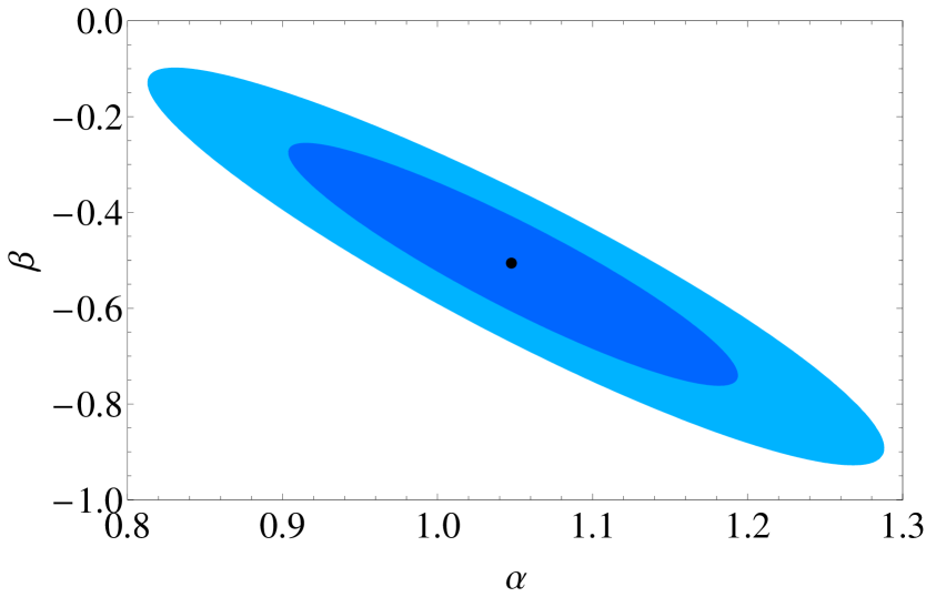
Figure 2: The 1$\sigma$ and 2$\sigma$ contours in the $(\alpha,\beta)$ plane for the 2 parameter model with $\gamma=0$. The black dot ($\alpha=1.05$, $\beta=-0.51$) corresponds to the best fit.

IV Results

We solve Eq. (5)-(6) numerically to find $r(z)$ for the matter-dominated model (SCDM). Then the model is tested against the SnIa data by using Eqs. (3), (15), and (16). Since the parameter $\gamma$ does not appear up to third order in the expansion of Eq. (10), we will also consider the case where $\gamma=0$.

In Fig. 1 (left) we present the best fit distance modulus versus the redshift $z$ for the best fit $\Lambda$CDM model (dashed line), with the present matter density parameter $\Omega_{\rm 0m}=0.289^{+0.023}_{-0.022}$) and the SCDM model + IR correction of Eq. (10) with all 3 parameters (solid black line) and the 2 parameter case with $\gamma=0$ (dotted line). For the two parameter case we find that $\alpha=1.05^{+0.15}_{-0.14}$ and $\beta=-0.51^{+0.23}_{-0.23}$ for a $\chi^{2}=464.031$ or a $\chi^{2}$ per degree of freedom $\sim 1.17$, whereas the best fit $\Lambda$CDM has a $\chi^{2}$ per degree of freedom $\sim 1.18$.

In Fig. 1 (right) we plot the residuals of our best fit relative to the $\Lambda$CDM model, i.e. the difference of $\mu_{\rm bestfit}(z)-\mu_{\Lambda{\rm CDM}}(z)$, for the model with the IR correction of Eq. (5) with all 3 parameters (solid black line) and the 2 parameter case and $\gamma=0$ (dotted line). In Fig. 2 we show the 1$\sigma$ and 2$\sigma$ contours for the parameters $\alpha$ and $\beta$ of Eq. (5) with $\gamma=0$. The black dot indicates the best-fit.

We should note that the two parameter model fits very well the data even if the exact numbers $\alpha=1$, $\beta=-1/2$ and $\gamma=0$ are used. In this case we find that $\chi^{2}=465.462$ and a $\chi^{2}$ per degree of freedom $\sim 1.18$, which is the same as the best fit $\Lambda$CDM model. The reason for this success of the model can be seen from the first of Eq. (II). The standard cosmological model predicts values of $w_{\rm eff}\simeq-1$ and $\Omega_{\rm DE}^{\rm eff}\simeq 0.7$, which gives $\alpha\simeq 1$. The value of $\beta\simeq-0.7$ derived from the second of Eqs. (II) is slightly different from its best fit $\beta\simeq-0.5$ because of the limitation of the expansion (10) valid only in the low redshift regime.

The original model of Ref. fedo , i.e. Eq. (2), corresponds to $\alpha=\beta=0$, $\gamma=1/4$. In this case, however, the agreement is not very good as the $\chi^{2}$ per degree of freedom is $\sim 2.21$ with the difference from the $\Lambda$CDM model being about $20\sigma$. This discrepancy can be explained by the fact that the IR correction does not kick in early enough to allow for good compatibility with the data, while in low redshifts the SCDM behavior of the model dominates. This latter property comes from the fact that the $\gamma$-dependent term appears only at the order of $z^{4}$ in Eq. (10).

If we consider all three parameters $\alpha$, $\beta$ and $\gamma$ to be free, then the best fit parameters are $\alpha=0.61$, $\beta=1.29$ and $\gamma=-1.51$ for a $\chi^{2}=459.424$ or a $\chi^{2}$ per degree of freedom $\sim 1.17$. As it can be seen in Fig. 1 (solid black line), the corresponding luminosity distance shows a more significant departure from $\Lambda$CDM at high redshift.

Finally, it is interesting to consider the case where we fix the parameters $\alpha$ and $\beta$ to the exact numbers $\alpha=1$, $\beta=-1/2$ and allow $\gamma$ to vary. In this case we expect that by changing $\gamma$ we will be able to improve $\chi^{2}$ and still be able to compare with $\Lambda$CDM as there will be only one free parameter in the model. The result is $\chi^{2}=465.082$ for $\gamma=0.052$, which is slightly worse ($\delta\chi^{2}\sim 1$) than the three parameter case, but it is slightly better ($\delta\chi^{2}\sim 0.5$) than $\Lambda$CDM ($\chi^{2}=465.513$ for $\Omega_{\rm 0m}=0.289$).

Table 1: Comparison of the one, two and three parameter models to $\Lambda$CDM. Note that the differences for the AIC and BIC are in both cases with regard to the model with the minimum value for the corresponding criterion. For the definition of the AIC and BIC, see Eqs. (17) and (18).

Model	AIC	$\Delta$AIC	BIC	$\Delta$BIC
$\Lambda$CDM	$467.513$	$2.089$	$471.497$	$0.000$
1 parameter	$467.082$	$1.658$	$471.066$	$-0.431$
2 parameters	$468.031$	$2.607$	$475.999$	$4.502$
3 parameters	$465.424$	$0.000$	$477.376$	$5.879$

In Table 1 we present the results of the two information criteria, the AIC and the BIC. According to the AIC the three parameter model is the best, with the $\Lambda$CDM having considerably less support, as the difference between the two is slightly larger than 2. On the contrary, using the BIC we find that the $\Lambda$CDM is now the best and also having positive evidence against the other models. In all cases, the two parameter model fairs moderately with both the AIC and the BIC.

V Conclusions

We have considered IR modifications of gravity that do not imply the presence of a new mass scale in the theory and we have studied their compatibility with the SnIa data. Our first result is that the mechanism derived in Ref. fedo (see also Appendix A), Eq. (1), is not enough, by itself, to describe the observed amount of acceleration. The absence of free parameters in equation (1) (the model in fedo has one parameter less than $\Lambda$CDM) does not make up for the very poor fit of the data. However, a more general structure of corrections (4) can lead to a sensibly larger luminosity distance than in the Einstein de Sitter universe. In particular, when $\gamma=0$ in Eq. (5)-(6), we have found that the model fits the data very well for the values close to the exact numbers $\alpha=1$ and $\beta=-1/2$. It is interesting to consider such sharp numerical values, not because of abstract numerology, but because a mechanism analogous to that described in Appendix A very naturally produces coefficients which are integers or simple fractions.

At present it is not clear if the corrections that one finds by applying USEP to a field automatically apply to, or are inherited by, other types of fields. The suggested luminosity distance may eventually turn out to be produced by considering other fields than the scalar field considered in fedo or by means of other theoretical insights. We also considered the full three parameters model (5)-(6), whose best fit considerably improves the $\chi^{2}$ and is found to be favored over $\Lambda$CDM by the AIC but not by the BIC criterion.

It should be noted that the parameters that we are fitting are not coupling constants, and do not appear in a Lagrangian. Rather, they are intended as the terms of a series expansion that approximate the new “IR-completed” theory starting from GR. As mentioned in the introduction, the proposed deformation is present at any time during the cosmological evolution; it affects any cosmological observation at high redshift, regardless of when such an observation takes place, and therefore addresses the “coincidence problem” in the most direct way.

We note that our model requires a rather low value of the Hubble constant, $H_{0}\sim 50$ km/s/Mpc, compared to the constraint from the Hubble Key Project with the determination of $H_{0}=72\pm 8$ km/s/Mpc Freedman . This comes from the fact that the Hubble parameter evolves as $H(z)\simeq H_{0}(1+z)^{3/2}$ even for $z\lesssim{\cal O}(1)$ due to the absence of a dark energy component. However, methods of the determination of $H_{0}$ that are largely independent of distance scales of the Large Magellanic Cloud Cepheid typically give low values of $H_{0}$ Sarkar . For example, Reese et al. Reese showed that Sunyaev-Zel’dovich distances to 41 clusters provide the constraint $H_{0}=54^{+4}_{-3}$ km/s/Mpc in the Einstein de Sitter universe. Thus the information of $H_{0}$ alone is not yet sufficient to rule out our model.

It would be interesting to see the effect of the proposed IR correction on the angular diameter distance to the last scattering surface and estimate the modification to the temperature anisotropies in Cosmic Microwave Background (CMB). CMB data will be certainly useful to place further constraints on our model and to complete the picture at higher redshift.

Appendix A USEP and the derivation of Eq. (1)

While referring to fedo for details and motivations, it is worth summarizing here the basic steps that lead to Eq. (1), based on the “ultra strong equivalence principle” (USEP). The USEP is a statement about the bare energy momentum tensor of the quantized fields on a general background, namely:

USEP: For each matter field or sector sufficiently decoupled from all other matter fields, there exists a state, the “vacuum”, for which the expectation value of the (bare) energy momentum tensor reads the same as in flat space, regardless of the configuration of the gravitational field.

Our starting point is a free scalar field with the action

$$S=\frac{1}{2}\int{\rm d}^{4}x\sqrt{-g}\left(\partial\phi^{2}-m^{2}\phi^{2}\right)\,,$$ (19)

in a spatially flat FLRW metric:

$${\rm d}s^{2}={\rm d}t^{2}-a^{2}(t){\rm d}\vec{x}^{2}\,.$$ (20)

The equations of motions of the field and the $00$ component of its energy momentum tensor read, respectively,

$$\ddot{\phi}(t,\vec{x})+3H\dot{\phi}(t,\vec{x})-\frac{\partial_{i}^{2}}{a(t)^{2}}\phi(t,\vec{x})+m^{2}\phi(t,\vec{x})=0,$$ (21)

$$T^{0}_{0}(t,\vec{x})=\frac{1}{2}\left[{\dot{\phi}}^{2}+\frac{1}{a^{2}}(\partial_{j}\phi)^{2}+m^{2}\phi^{2}\right].$$ (22)

In order to apply USEP we now review the standard calculation of the energy momentum VEV in such a spacetime and compare it to the flat space result.

Upon standard quantization in the Heisenberg picture the field is expanded in creators and annihilators:

$$\phi(t,\vec{x})=\int{\rm d}n^{3}\left[\psi_{n}(t)e^{i\vec{n}\cdot\vec{x}}A_{\vec{n}}+\psi^{*}_{n}(t)e^{-i\vec{n}\cdot\vec{x}}A^{\dagger}_{\vec{n}}\right]\,,$$ (23)

where $\vec{n}$ is the comoving momentum label in the FLRW space; $\vec{n}$ is a conserved quantity, related to the proper physical momentum $\vec{p}$ by $\vec{p}=\vec{n}/a(t)$. From the canonical commutation relations $[\phi(\vec{x}),\pi(\vec{x}\,^{\prime})]=i(2\pi)^{3}\delta^{3}(\vec{x}-\vec{x}\,^{\prime})$, the commutation relations among the global Fourier operators are easily derivable,

$$[A_{\vec{n}},A^{\dagger}_{\vec{n}^{\prime}}]=\delta^{3}(\vec{n}-\vec{n}\,^{\prime})\,.$$ (24)

It is customary to choose $A_{\vec{n}}$ as the operator that always annihilates the vacuum. The chosen vacuum state is therefore implicitly characterized by the choice of the mode functions $\psi_{n}(t)$, that, by (23) and (21), satisfy

$$\ddot{\psi}_{n}+3H\dot{\psi}_{n}+\omega_{n}^{2}\psi_{n}=0,$$ (25)

where $\omega_{n}=\sqrt{n^{2}/a^{2}+m^{2}}$.

The solutions of (25) corresponding to the adiabatic vacuum birrell ; fullings can be found by a formal WKB expansion. After quantization, the energy momentum tensor of the field (22) becomes an operator whose expectation value on the adiabatic vacuum reads fullings ; fedo

$$\langle T_{0}^{0}(t,\vec{x})\rangle=\frac{1}{4\pi^{2}a^{3}}\int_{0}^{\infty}n^{2}\left[\omega_{n}+\frac{H^{2}a}{2n}+{\cal O}(n^{-3})\right]\,{\rm d}n\,.$$ (26)

The above should be compared to the flat space result

$$\langle T_{0}^{0}(t,\vec{x})\rangle_{\rm flat}=\frac{1}{4\pi^{2}a^{3}}\int_{0}^{\infty}n^{2}\omega_{n}\,{\rm d}n\,.$$ (27)

It is known that there is a strict connection between the geometric properties of a manifold and the spectrum of the differential operators heat or the algebra of functions connes therein defined; such abstract characterizations have occasionally been used for generalizing common geometrical concepts and the description of spacetime itself connes ; sw . However, so far, attempts in this direction have always been applied to the UV and intended to modify spacetime at the smallest scales. Here we would like to modify the IR-spectral properties of the FLRW metric (and therefore its geometry) in order to enforce USEP. The proposed deformation is argued to correspond to a breakdown of the metric Riemannian structure at distances comparable to $H^{-1}$.

So the idea is to modify the physics in the infra-red but strictly maintain the equations and the relations valid locally such as the field equations (21) and the form of the energy momentum tensor (22). We choose a point in FLRW ($\vec{x}=0$) and make a formal Taylor expansion of which GR is the zeroth order. In the spirit of a general spectral deformation, we conjecture a mismatch between the “metric-manifold” Fourier labels $\vec{n}$ and the physical momenta $\vec{k}$ that locally define the infinitesimal translations and the derivatives of the local fields. In other words, we now write the field in $\vec{x}\simeq 0$ as

$$\phi(t,\vec{x}\approx 0)=\int{\rm d}n^{3}\left[\psi_{k}(t)e^{i\vec{k}\cdot\vec{x}}A_{\vec{n}}+\psi^{*}_{k}(t)e^{-i\vec{k}\cdot\vec{x}}A^{\dagger}_{\vec{n}}\right]\,,$$ (28)

where

$$\vec{k}=\vec{n}\left(1-\frac{H^{2}a^{2}}{2n^{2}}+{\rm higher\ order}\right)\,.$$ (29)

Note that, when derivatives of the field are taken in $\vec{x}=0$, a factor of $k$, instead of $n$, drops. The form of above relation, which is one of the main results of fedo , is dictated by the request that the quadratically divergent time dependent piece of (26) disappears. In other words, that is the first order correction in order to impose USEP upon this particular GR solution. The corrected mode equation is in fact obtained by substituting (28) into (21), which is assumed to be strictly valid because it applies locally. To the modified mode equation, $\ddot{\psi}_{k}(t)+3H\dot{\psi}_{k}(t)+\omega^{2}_{k}\psi_{k}(t)=0$, the same WKB expansion can be applied and the quadratic divergence in (26) is reabsorbed just by re-expressing $\langle 0|\,T_{0}^{0}|0\rangle$ in terms of the appropriate “flat measure” time-independent Fourier coordinates $n$:

$$\langle T_{0}^{0}(t,\vec{x}\approx 0)\rangle\!\! = \!\!\frac{1}{4\pi^{2}a^{3}}\int_{0}^{\infty}n^{2}\left[\omega_{k}+\frac{H^{2}a}{2k}+{\cal O}(n^{-3})\right]\,{\rm d}n$$

$$= \frac{1}{4\pi^{2}a^{3}}\int_{0}^{\infty}n^{2}\left[\omega_{n}+{\cal O}(n^{-3})\right]\,{\rm d}n\,.$$

In order to define local quantities away from the origin we exploit the assumption of spatial homogeneity and use the translation operator

$$T(\vec{\lambda})=\exp\left({-i\vec{\lambda}\cdot\int d^{3}n\,\vec{k}(\vec{n})\,A^{\dagger}_{\vec{n}}A_{\vec{n}}}\right)\,,$$ (30)

that we obtain by simple exponentiation of the (modified!) momentum operator. The parameter $\lambda$ is the comoving distance. The field away from $\vec{x}=0$ is thus defined as $\phi(t,\vec{\lambda})\equiv T_{i}(\lambda)\,\phi(t,0)\,T_{i}^{-1}(\lambda)$ and reads

$$\phi(t,\vec{\lambda})=\int{\rm d}^{3}n\,\left[\psi_{k}(t)e^{i\vec{k}\cdot\vec{\lambda}}A_{\vec{n}}+\psi^{*}_{k}(t)e^{-i\vec{k}\cdot\vec{\lambda}}A^{\dagger}_{\vec{n}}\right].$$ (31)

From the above expression it is straightforward to calculate the modified commutator between the canonical momentum $\pi(0)=a^{3}{\dot{\phi}}(0)$ and the field at comoving distance $\vec{\lambda}$,

$$[\pi(0),\phi(\vec{\lambda})]=-i\left(\delta^{3}(\vec{\lambda})+\frac{1}{8\pi}\frac{H^{2}a^{2}}{\lambda}\right).$$ (32)

Note that there is a potential ambiguity in defining the time derivative of a displaced operator. By deriving (31) we get

$$\pi(\vec{\lambda})\!\! = \!\!a^{3}\int{\rm d}^{3}n\,\left[\dot{\psi}_{k}(t)e^{i\vec{k}\cdot\vec{\lambda}}A_{\vec{n}}+\dot{\psi}^{*}_{k}(t)e^{-i\vec{k}\cdot\vec{\lambda}}A^{\dagger}_{\vec{n}}\right]$$

$$+ ia^{3}\int{\rm d}^{3}n\,(\vec{k}\cdot\vec{\lambda})\dot{}\ \left[\psi_{k}\ e^{i\vec{k}\cdot\vec{\lambda}}A_{\vec{n}}-\psi^{*}_{k}\ e^{-i\vec{k}\cdot\vec{\lambda}}A^{\dagger}_{\vec{n}}\right].$$

The second line in the above equation is there because $k$ is time dependent. However, if we just apply the translation to $\pi(0)$, instead of deriving $\phi(\vec{\lambda})$, those terms would not be there. Therefore, for consistency, we need to make them ineffective at the required order of approximation. This can be done by imposing that $[\phi(0),\pi(\vec{\lambda})]=-[\pi(0),\phi(\vec{\lambda})]$. Because of the second line the last equation, the commutator between $\phi(0)$ and $\pi(\lambda)$ gives

$$[\phi(0),\pi(\vec{\lambda})] = -[\pi(0),\phi(\vec{\lambda})]$$

$$-2i\frac{a^{3}}{(2\pi)^{3}}\int{\rm d}^{3}n\,e^{-i\vec{k}\cdot\vec{\lambda}}\left|\psi_{n}\right|^{2}(\vec{k}\cdot\vec{\lambda})\dot{}\,,$$

the last term being the spurious contribution. In order to get rid of it, we have to make the comoving physical distance $\vec{\lambda}$ also time dependent. This effectively means that, after an infinitesimal time step ${\rm d}t$, we have to reconsider the field translated, from $\vec{x}\approx 0$, not by the same comoving distance $\lambda$, but by a slightly different amount.

At high momenta/small distances, since $|\psi_{k}|^{2}\sim 1/n$, the integral in the second term of (A) reads

$$\int{\rm d}^{3}n\,e^{-i\vec{n}\cdot\vec{\lambda}}\,\frac{1}{n}\left[\dot{\vec{\lambda}}\cdot\vec{n}\left(1-\frac{H^{2}a^{2}}{2n^{2}}\right)-\vec{\lambda}\cdot\vec{n}\frac{(H^{2}a^{2})\dot{}}{2n^{2}}\right]\,.$$

We make the ansatz $\dot{\vec{\lambda}}=b\lambda^{2}(H^{2}a^{2})\dot{}\,\vec{\lambda}$, where $b$ is a number to be determined. We get

$$\int{\rm d}^{3}n\,e^{-i\vec{k}\cdot\vec{\lambda}}\left|\psi_{n}\right|^{2}(\vec{k}\cdot\vec{\lambda})\dot{}\$$

$$\simeq \ i(H^{2}a^{2})\dot{}\ \frac{d}{d\alpha}\int d^{3}n\,\left.\left(\frac{b\lambda^{2}}{n}-\frac{1}{2n^{3}}\right)e^{-i\alpha\,\vec{n}\cdot\vec{\lambda}}\right|_{\alpha=1}.$$

The last integral can be regularized by setting $n^{-3}\rightarrow n^{-3+\epsilon}$ and taking the $\epsilon\rightarrow 0$ limit only after deriving with respect to $\alpha$. The result is null for $b=1/4$, which fixes the time dependence of $\lambda$:

$$\dot{\lambda}=\lambda^{3}\frac{(H^{2}a^{2})\dot{}}{4}.$$ (34)

Appendix B Exact solutions

Here we present some analytical solutions for the differential equation (5). If $\gamma=0$ we obtain the following analytic solution:

$$H_{0}r(z)=\frac{4/\sqrt{1+z}}{-1-2\alpha+\sqrt{\delta}+2\sqrt{\delta}/[(1+z)^{\sqrt{\delta}/2}-1]}\,,$$ (35)

where $\delta=(1+2\alpha)^{2}-16\beta$.

When $\gamma\neq 0$, finding the solution is much more difficult and can only be given in an implicit form. For example, let us consider the correction in Eq. (2), i.e. $\alpha=\beta=0$ and $\gamma=1/4$. Setting $R(z)\equiv r(z)\sqrt{1+z}$, we get a differential equation for the function $R(z)$:

$$\frac{{\rm d}R(z)}{{\rm d}z}=\frac{1}{1+z}+\frac{R(z)}{2(1+z)}+\frac{R(z)^{3}}{4(1+z)}\,,$$ (36)

with initial conditions $R(0)=0$ and $({\rm d}R/{\rm d}z)(0)=1$. By direct differentiation it can be shown that the solution to Eq. (36) is given in an implicit form by:

$$z = -1+\left(\frac{R(z)}{x_{1}}-1\right)^{\frac{4}{2+3x_{1}^{2}}}\left(\frac{R(z)}{x_{2}}-1\right)^{\frac{4}{2+3x_{2}^{2}}}$$ (37)

$$\,\,\,\,\,\,\,\,\,\times\left(\frac{R(z)}{x_{3}}-1\right)^{\frac{4}{2+3x_{3}^{2}}}\,,$$

where the parameters $x_{1},x_{2},x_{3}$ are the roots of the polynomial equation:

$$4+2x_{i}+x_{i}^{3}=0\,.$$ (38)

When all three parameters $\alpha$, $\beta$, and $\gamma$ are not zero, then we can still find an implicit solution for $r(z)$ but in this case it is very complicated, so we will not reproduce it here.

References

- (1) A. G. Riess et al., Astron. J. 116, 1009 (1998); Astron. J. 117, 707 (1999); S. Perlmutter et al., Astrophys. J. 517, 565 (1999).
- (2) D. N. Spergel et al., Astrophys. J. Suppl. 148, 175 (2003); Astrophys. J. Suppl. 170, 377 (2007); E. Komatsu et al., Astrophys. J. Suppl. 180, 330 (2009).
- (3) D. J. Eisenstein et al. [SDSS Collaboration], Astrophys. J. 633, 560 (2005); W. J. Percival et al., Mon. Not. Roy. Astron. Soc. 381, 1053 (2007).
- (4) V. Sahni and A. A. Starobinsky, Int. J. Mod. Phys. D 9, 373 (2000); S. M. Carroll, Living Rev. Rel. 4, 1 (2001); T. Padmanabhan, Phys. Rept. 380, 235 (2003); P. J. E. Peebles and B. Ratra, Rev. Mod. Phys. 75, 559 (2003); E. J. Copeland, M. Sami and S. Tsujikawa, Int. J. Mod. Phys. D 15, 1753 (2006); L. Perivolaropoulos, AIP Conf. Proc. 848, 698 (2006); L. Amendola and S. Tsujikawa, Dark energy–Theory and Observations, Cambridge University press (2010), in press.
- (5) B. Ratra and J. Peebles, Phys. Rev D 37, 321 (1988).
- (6) P. J. Steinhardt, L. M. Wang and I. Zlatev, Phys. Rev. D 59, 123504 (1999).
- (7) G. R. Dvali, G. Gabadadze and M. Porrati, Phys. Lett. B 485, 208 (2000); C. Deffayet, G. R. Dvali and G. Gabadadze, Phys. Rev. D 65, 044023 (2002).
- (8) N. Arkani-Hamed, S. Dimopoulos, G. Dvali and G. Gabadadze, arXiv:hep-th/0209227; G. Dvali, S. Hofmann and J. Khoury, Phys. Rev. D 76, 084006 (2007); C. de Rham, S. Hofmann, and A. J. Tolley, JCAP 0802, 011 (2008).
- (9) G. Dvali and J. Khoury, private communications.
- (10) W. Hu and I. Sawicki, Phys. Rev. D 76, 064004 (2007); A. A. Starobinsky, JETP Lett. 86, 157 (2007); S. A. Appleby and R. A. Battye, Phys. Lett. B 654, 7 (2007); S. Tsujikawa, Phys. Rev. D 77, 023507 (2008).
- (11) L. Amendola, R. Gannouji, D. Polarski and S. Tsujikawa, Phys. Rev. D 75, 083504 (2007); B. Li and J. D. Barrow, Phys. Rev. D 75, 084010 (2007); L. Amendola and S. Tsujikawa, Phys. Lett. B 660, 125 (2008).
- (12) K. Tomita, Mon. Not. Roy. Astron. Soc. 326, 287 (2001); M. N. Celerier, Astron. Astrophys. 353, 63 (2000); H. Iguchi, T. Nakamura and K. i. Nakao, Prog. Theor. Phys. 108, 809 (2002).
- (13) S. Rasanen, JCAP 0402, 003 (2004); E. W. Kolb, S. Matarrese, A. Notari and A. Riotto, Phys. Rev. D 71, 023524 (2005); M. Gasperini, G. Marozzi and G. Veneziano, JCAP 0903, 011 (2009).
- (14) F. Piazza, Int. J. Mod. Phys. D 18, 2181 (2009) [arXiv:0904.4299 [hep-th]]; see also F. Piazza, arXiv:0910.4677 [gr-qc].
- (15) F. Piazza, New J. Phys. 11, 113050 (2009) [arXiv:0907.0765 [hep-th]].
- (16) L. Amendola, M. Gasperini and F. Piazza, JCAP 0409, 014 (2004); Phys. Rev. D 74, 127302 (2006).
- (17) M. Hicken et al., Astrophys. J. 700, 1097 (2009).
- (18) M. Kowalski et al., Astrophys. J. 686, 749 (2008).
- (19) S. Nesseris and L. Perivolaropoulos, JCAP 0701, 018 (2007).
- (20) S. Nesseris and L. Perivolaropoulos, Phys. Rev. D 72, 123519 (2005).
- (21) S. Nesseris and L. Perivolaropoulos, Phys. Rev. D 70, 043531 (2004).
- (22) A. R. Liddle, Mon. Not. Roy. Astron. Soc. 351, L49 (2004).
- (23) M. Biesiada, JCAP 0702, 003 (2007).
- (24) F. R. Urban and A. R. Zhitnitsky, arXiv:0909.2684 [astro-ph.CO]; F. R. Urban and A. R. Zhitnitsky, Phys. Rev. D 80, 063001 (2009).
- (25) W. L. Freedman et al. [HST Collaboration], Astrophys. J. 553, 47 (2001).
- (26) A. Blanchard, M. Douspis, M. Rowan-Robinson and S. Sarkar, Astron. Astrophys. 412, 35 (2003).
- (27) E. D. Reese, J. E. Carlstrom, M. Joy, J. J. Mohr, L. Grego and W. L. Holzapfel, Astrophys. J. 581, 53 (2002).
- (28) N. D. Birrell and P. C. W. Davies, “Quantum Fields In Curved Space,” Cambridge University Press, 340p (1982).
- (29) Y. B. Zeldovich and A. A. Starobinsky, Sov. Phys. JETP 34, 1159 (1972) [Zh. Eksp. Teor. Fiz. 61, 2161 (1971)]; L. Parker and S. A. Fulling, Phys. Rev. D 9, 341 (1974); S. A. Fulling and L. Parker, Annals Phys. 87, 176 (1974).
- (30) D. V. Vassilevich, Phys. Rept. 388, 279 (2003).
- (31) A. Connes, “Noncommutative geometry,” Academic Press, San Diego, CA (1994).
- (32) N. Seiberg and E. Witten, JHEP 9909, 032 (1999).