Magnetic field decay of three interlocked flux rings with zero linking number

Abstract

The resistive decay of chains of three interlocked magnetic flux rings is considered. Depending on the relative orientation of the magnetic field in the three rings, the late-time decay can be either fast or slow. Thus, the qualitative degree of tangledness is less important than the actual value of the linking number or, equivalently, the net magnetic helicity. Our results do not suggest that invariants of higher order than that of the magnetic helicity need to be considered to characterize the decay of the field.

I Introduction

Magnetic helicity plays an important role in plasma physics Tay74 ; JC84 ; BF84 , solar physics Low96 ; RK94 ; RK96 , cosmology BEO96 ; FC00 ; CHB05 , and dynamo theory PFL76 ; BS05 . This is connected with the fact that magnetic helicity is a conserved quantity in ideal magnetohydrodynamics Wol58 . The conservation law of magnetic helicity is ultimately responsible for inverse cascade behavior that can be relevant for spreading primordial magnetic field over large length scales. It is also likely the reason why the magnetic fields of many astrophysical bodies have length scales that are larger than those of the turbulent motions responsible for driving these fields. In the presence of finite magnetic diffusivity, the magnetic helicity can only change on a resistive time scale. Of course, astrophysical bodies are open, so magnetic helicity can change by magnetic helicity fluxes out of or into the domain of interest. However, such cases will not be considered in the present paper.

In a closed or periodic domain without external energy supply, the decay of a magnetic field depends critically on the value of the magnetic helicity. This is best seen by considering spectra of magnetic energy and magnetic helicity. The magnetic energy spectrum $M(k)$ is normalized such that

$$\int M(k)\,dk=\langle\mathchoice{\mbox{\boldmath$\displaystyle B$}}{\mbox{\boldmath$\textstyle B$}}{\mbox{\boldmath$\scriptstyle B$}}{\mbox{\boldmath$\scriptscriptstyle B$}}{}^{2}\rangle/2\mu_{0},$$ (1)

where $\textstyle B$ is the magnetic field, $\mu_{0}$ is the magnetic permeability, and $k$ is the wave number (ranging from 0 to $\infty$). The magnetic helicity spectrum $H(k)$ is normalized such that

$$\int H(k)\,dk=\langle\mathchoice{\mbox{\boldmath$\displaystyle A$}}{\mbox{\boldmath$\textstyle A$}}{\mbox{\boldmath$\scriptstyle A$}}{\mbox{\boldmath$\scriptscriptstyle A$}}{}\cdot\mathchoice{\mbox{\boldmath$\displaystyle B$}}{\mbox{\boldmath$\textstyle B$}}{\mbox{\boldmath$\scriptstyle B$}}{\mbox{\boldmath$\scriptscriptstyle B$}}{}\rangle,$$ (2)

where $\textstyle A$ is the magnetic vector potential with $\mathchoice{\mbox{\boldmath$\displaystyle B$}}{\mbox{\boldmath$\textstyle B$}}{\mbox{\boldmath$\scriptstyle B$}}{\mbox{\boldmath$\scriptscriptstyle B$}}{}=\mathchoice{\mbox{\boldmath$\displaystyle\nabla$}}{\mbox{\boldmath$\textstyle\nabla$}}{\mbox{\boldmath$\scriptstyle\nabla$}}{\mbox{\boldmath$\scriptscriptstyle\nabla$}}{}\times\mathchoice{\mbox{\boldmath$\displaystyle A$}}{\mbox{\boldmath$\textstyle A$}}{\mbox{\boldmath$\scriptstyle A$}}{\mbox{\boldmath$\scriptscriptstyle A$}}{}$. In a closed or periodic domain, $H(k)$ is gauge-invariant, i.e. it does not change after adding a gradient term to $\textstyle A$. For finite magnetic helicity, the magnetic energy spectrum is bound from below Wol58 such that

$$M(k)\geq k|H(k)|/2\mu_{0}.$$ (3)

This relation is also known as the realizability condition Mof69 . Thus, the decay of a magnetic field is subject to a corresponding decay of its associated magnetic helicity. Given that in a closed or periodic domain the magnetic helicity changes only on resistive time scales Ber84 , the decay of magnetic energy is slowed down correspondingly. More detailed statements can be made about the decay of turbulent magnetic fields, where the energy decays in a power-law fashion proportional to $t^{-\sigma}$. In the absence of magnetic helicity, $\langle\mathchoice{\mbox{\boldmath$\displaystyle A$}}{\mbox{\boldmath$\textstyle A$}}{\mbox{\boldmath$\scriptstyle A$}}{\mbox{\boldmath$\scriptscriptstyle A$}}{}\cdot\mathchoice{\mbox{\boldmath$\displaystyle B$}}{\mbox{\boldmath$\textstyle B$}}{\mbox{\boldmath$\scriptstyle B$}}{\mbox{\boldmath$\scriptscriptstyle B$}}{}\rangle=0$, we have a relatively rapid decay with $\sigma\approx 1.3$ MacLow , while with $\langle\mathchoice{\mbox{\boldmath$\displaystyle A$}}{\mbox{\boldmath$\textstyle A$}}{\mbox{\boldmath$\scriptstyle A$}}{\mbox{\boldmath$\scriptscriptstyle A$}}{}\cdot\mathchoice{\mbox{\boldmath$\displaystyle B$}}{\mbox{\boldmath$\textstyle B$}}{\mbox{\boldmath$\scriptstyle B$}}{\mbox{\boldmath$\scriptscriptstyle B$}}{}\rangle\neq 0$, the decay is slower with $\sigma$ between 1/2 CHB05 and 2/3 BM99 .

The fact that the decay is slowed down in the helical case is easily explained in terms of the topological interpretation of magnetic helicity. It is well known that the magnetic helicity can be expressed in terms of the linking number $n$ of discrete magnetic flux ropes via Mof69

$$\int\mathchoice{\mbox{\boldmath$\displaystyle A$}}{\mbox{\boldmath$\textstyle A$}}{\mbox{\boldmath$\scriptstyle A$}}{\mbox{\boldmath$\scriptscriptstyle A$}}{}\cdot\mathchoice{\mbox{\boldmath$\displaystyle B$}}{\mbox{\boldmath$\textstyle B$}}{\mbox{\boldmath$\scriptstyle B$}}{\mbox{\boldmath$\scriptscriptstyle B$}}{}\,{\rm d}{}V=2n\Phi_{1}\Phi_{2},$$ (4)

where

$$\Phi_{i}=\int_{S_{i}}\mathchoice{\mbox{\boldmath$\displaystyle B$}}{\mbox{\boldmath$\textstyle B$}}{\mbox{\boldmath$\scriptstyle B$}}{\mbox{\boldmath$\scriptscriptstyle B$}}{}\cdot{\rm d}{}\mathchoice{\mbox{\boldmath$\displaystyle S$}}{\mbox{\boldmath$\textstyle S$}}{\mbox{\boldmath$\scriptstyle S$}}{\mbox{\boldmath$\scriptscriptstyle S$}}{}\quad\mbox{(for $i=1$ and 2)}$$ (5)

are the magnetic fluxes of the two ropes with cross-sectional areas $S_{1}$ and $S_{2}$. The slowing down of the decay is then plausibly explained by the fact that a decay of magnetic energy is connected with a decay of magnetic helicity via the realizability condition (3). Thus, a decay of magnetic helicity can be achieved either by a decay of the magnetic flux or by magnetic reconnection. Magnetic flux can decay through annihilation with oppositely oriented flux. Reconnection on the other hand reflects a change in the topological connectivity, as demonstrated in detail in Ref. (PriestRecon2000, , p.28).

The situation becomes more interesting when we consider a flux configuration that is interlocked, but with zero linking number. This can be realized quite easily by considering a configuration of two interlocked flux rings where a third flux ring is connected with one of the other two rings such that the total linking number becomes either 0 or 2, depending on the relative orientation of the additional ring, as is illustrated in Fig. 1. Topologically, the configuration with linking numbers of 0 and 2 are the same except that the orientation of the field lines in the upper ring is reversed. Nevertheless, the simple topological interpretation becomes problematic in the case of zero linking number, because then also the magnetic helicity is zero, so the bound of $M$ from below disappears, and $M$ can now in principle freely decay to zero. One might expect that the topology should then still be preserved, and that the linking number as defined above, which is a quadratic invariant, should be replaced with a higher order invariant RA94 ; HM02 ; Kom09 . It is also possible that in a topologically interlocked configuration with zero linking number the magnetic helicity spectrum $H(k)$ is still finite and that bound (3) may still be meaningful. In order to address these questions we perform numerical simulations of the resistive magnetohydrodynamic equations using simple interlocked flux configurations as initial conditions. We also perform a control run with a non-interlocked configuration and zero helicity in order to compare the magnetic energy decay with the interlocked case.

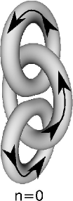
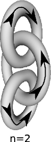
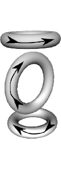
Figure 1: Visualization of the triple ring configuration at the initial time. Arrows indicate the direction of the field lines in the rings, corresponding to a configuration with $n=0$ (left) and $n=2$ (center). On the right the non-interlocked configuration with $n=0$ is shown.

Magnetic helicity evolution is independent of the equation of state and applies hence to both compressible and incompressible cases. In agreement with earlier work KB99 we assume an isothermal gas, where pressure is proportional to density and the sound speed is constant. However, in all cases the bulk motions stay subsonic, so for all practical purposes our calculations can be considered nearly incompressible, which would be an alternative assumption that is commonly made GM00 .

II Model

We perform simulations of the resistive magnetohydrodynamic equations for a compressible isothermal gas where the pressure is given by $p=\rho c_{\rm s}^{2}$, with $\rho$ being the density and $c_{\rm s}$ being the isothermal sound speed. We solve the equations for $\textstyle A$, the velocity $\textstyle U$, and the logarithmic density $\ln\rho$ in the form

$${\partial\mathchoice{\mbox{\boldmath$\displaystyle A$}}{\mbox{\boldmath$\textstyle A$}}{\mbox{\boldmath$\scriptstyle A$}}{\mbox{\boldmath$\scriptscriptstyle A$}}{}\over\partial t}=\mathchoice{\mbox{\boldmath$\displaystyle U$}}{\mbox{\boldmath$\textstyle U$}}{\mbox{\boldmath$\scriptstyle U$}}{\mbox{\boldmath$\scriptscriptstyle U$}}{}\times\mathchoice{\mbox{\boldmath$\displaystyle B$}}{\mbox{\boldmath$\textstyle B$}}{\mbox{\boldmath$\scriptstyle B$}}{\mbox{\boldmath$\scriptscriptstyle B$}}{}+\eta\nabla^{2}\mathchoice{\mbox{\boldmath$\displaystyle A$}}{\mbox{\boldmath$\textstyle A$}}{\mbox{\boldmath$\scriptstyle A$}}{\mbox{\boldmath$\scriptscriptstyle A$}}{},$$ (6)

$${{\rm D}{}\mathchoice{\mbox{\boldmath$\displaystyle U$}}{\mbox{\boldmath$\textstyle U$}}{\mbox{\boldmath$\scriptstyle U$}}{\mbox{\boldmath$\scriptscriptstyle U$}}{}\over{\rm D}{}t}=-c_{\rm s}^{2}\mathchoice{\mbox{\boldmath$\displaystyle\nabla$}}{\mbox{\boldmath$\textstyle\nabla$}}{\mbox{\boldmath$\scriptstyle\nabla$}}{\mbox{\boldmath$\scriptscriptstyle\nabla$}}{}\ln\rho+\mathchoice{\mbox{\boldmath$\displaystyle J$}}{\mbox{\boldmath$\textstyle J$}}{\mbox{\boldmath$\scriptstyle J$}}{\mbox{\boldmath$\scriptscriptstyle J$}}{}\times\mathchoice{\mbox{\boldmath$\displaystyle B$}}{\mbox{\boldmath$\textstyle B$}}{\mbox{\boldmath$\scriptstyle B$}}{\mbox{\boldmath$\scriptscriptstyle B$}}{}/\rho+\mathchoice{\mbox{\boldmath$\displaystyle F$}}{\mbox{\boldmath$\textstyle F$}}{\mbox{\boldmath$\scriptstyle F$}}{\mbox{\boldmath$\scriptscriptstyle F$}}{}_{\rm visc},$$ (7)

$${{\rm D}{}\ln\rho\over{\rm D}{}t}=-\mathchoice{\mbox{\boldmath$\displaystyle\nabla$}}{\mbox{\boldmath$\textstyle\nabla$}}{\mbox{\boldmath$\scriptstyle\nabla$}}{\mbox{\boldmath$\scriptscriptstyle\nabla$}}{}\cdot\mathchoice{\mbox{\boldmath$\displaystyle U$}}{\mbox{\boldmath$\textstyle U$}}{\mbox{\boldmath$\scriptstyle U$}}{\mbox{\boldmath$\scriptscriptstyle U$}}{},$$ (8)

where $\mathchoice{\mbox{\boldmath$\displaystyle F$}}{\mbox{\boldmath$\textstyle F$}}{\mbox{\boldmath$\scriptstyle F$}}{\mbox{\boldmath$\scriptscriptstyle F$}}{}_{\rm visc}=\rho^{-1}\mathchoice{\mbox{\boldmath$\displaystyle\nabla$}}{\mbox{\boldmath$\textstyle\nabla$}}{\mbox{\boldmath$\scriptstyle\nabla$}}{\mbox{\boldmath$\scriptscriptstyle\nabla$}}{}\cdot 2\nu\rho\bm{\mathsf{S}}$ is the viscous force, $\bm{\mathsf{S}}$ is the traceless rate of strain tensor, with components ${\sf S}_{ij}={\textstyle{1\over 2}}(U_{i,j}+U_{j,i})-{\textstyle{1\over 3}}\delta_{ij}\mathchoice{\mbox{\boldmath$\displaystyle\nabla$}}{\mbox{\boldmath$\textstyle\nabla$}}{\mbox{\boldmath$\scriptstyle\nabla$}}{\mbox{\boldmath$\scriptscriptstyle\nabla$}}{}\cdot\mathchoice{\mbox{\boldmath$\displaystyle U$}}{\mbox{\boldmath$\textstyle U$}}{\mbox{\boldmath$\scriptstyle U$}}{\mbox{\boldmath$\scriptscriptstyle U$}}{}$, $\mathchoice{\mbox{\boldmath$\displaystyle J$}}{\mbox{\boldmath$\textstyle J$}}{\mbox{\boldmath$\scriptstyle J$}}{\mbox{\boldmath$\scriptscriptstyle J$}}{}=\mathchoice{\mbox{\boldmath$\displaystyle\nabla$}}{\mbox{\boldmath$\textstyle\nabla$}}{\mbox{\boldmath$\scriptstyle\nabla$}}{\mbox{\boldmath$\scriptscriptstyle\nabla$}}{}\times\mathchoice{\mbox{\boldmath$\displaystyle B$}}{\mbox{\boldmath$\textstyle B$}}{\mbox{\boldmath$\scriptstyle B$}}{\mbox{\boldmath$\scriptscriptstyle B$}}{}/\mu_{0}$ is the current density, $\nu$ is the kinematic viscosity, and $\eta$ is the magnetic diffusivity.

The initial magnetic field is given by a suitable arrangement of magnetic flux ropes, as already illustrated in Fig. 1. These ropes have a smooth Gaussian cross-sectional profile that can easily be implemented in terms of the magnetic vector potential. We use the Pencil Code (http://pencil-code.googlecode.com), where this initial condition for $\textstyle A$ is already prepared, except that now we adopt a configuration consisting of three interlocked flux rings (Fig. 1) where the linking number can be chosen to be either 0 or 2, depending only on the field orientation in the last (or the first) of the three rings. Here, the two outer rings have radii $R_{\rm o}$, while the inner ring is slightly bigger and has the radius $R_{\rm i}=1.2R_{\rm o}$, but with the same flux. We use $R_{\rm o}$ as our unit of length. The sound travel time is given by $T_{\rm s}=R_{\rm o}/c_{\rm s}$.

In the initial state we have $\mathchoice{\mbox{\boldmath$\displaystyle U$}}{\mbox{\boldmath$\textstyle U$}}{\mbox{\boldmath$\scriptstyle U$}}{\mbox{\boldmath$\scriptscriptstyle U$}}{}=\bm{0}$ and $\rho=\rho_{0}=1$. Our initial flux, $\Phi=\int\mathchoice{\mbox{\boldmath$\displaystyle B$}}{\mbox{\boldmath$\textstyle B$}}{\mbox{\boldmath$\scriptstyle B$}}{\mbox{\boldmath$\scriptscriptstyle B$}}{}\cdot{\rm d}{}\mathchoice{\mbox{\boldmath$\displaystyle S$}}{\mbox{\boldmath$\textstyle S$}}{\mbox{\boldmath$\scriptstyle S$}}{\mbox{\boldmath$\scriptscriptstyle S$}}{}$, is the same for all tubes with $\Phi=0.1\,c_{\rm s}R_{\rm o}^{2}\sqrt{\mu_{0}\rho_{0}}$. This is small enough for compressibility effects to be unimportant, so the subsequent time evolution is not strongly affected by this choice. For this reason, the Alfvén time, $T_{\rm A}=\sqrt{\mu_{0}\rho_{0}}R_{\rm o}^{3}/\Phi$, will be used as our time unit. In all our cases we have $T_{\rm A}=10T_{\rm s}$ and denote the dimensionless time as $\tau=t/T_{\rm A}$. In all cases we assume that the magnetic Prandtl number, $\nu/\eta$, is unity, and we choose $\nu=\eta=10^{-4}R_{\rm o}c_{\rm s}=10^{-3}R_{\rm o}^{2}/T_{\rm A}$. We use $256^{3}$ mesh points.

We have chosen a fully compressible code, because it is readily available to us. Alternatively, as discussed at the end of § I, one could have chosen an incompressible code by ignoring the continuity equation and computing the pressure such that $\mathchoice{\mbox{\boldmath$\displaystyle\nabla$}}{\mbox{\boldmath$\textstyle\nabla$}}{\mbox{\boldmath$\scriptstyle\nabla$}}{\mbox{\boldmath$\scriptscriptstyle\nabla$}}{}\cdot\mathchoice{\mbox{\boldmath$\displaystyle U$}}{\mbox{\boldmath$\textstyle U$}}{\mbox{\boldmath$\scriptstyle U$}}{\mbox{\boldmath$\scriptscriptstyle U$}}{}=0$ at all times. Such an operation breaks the locality of the physics and is computationally more intensive, because it requires global communication.

III Results

Let us first discuss the visual appearance of the three interlocked flux rings at different times. In Fig. 2 we compare the three rings for the zero and finite magnetic helicity cases at the initial time and at $\tau=0.5$. Note that each ring shrinks as a result of the tension force. This effect is strongest in the core of each ring, causing the rings to show a characteristic indentation that was also seen in earlier inviscid and non-resistive simulations of two interlocked flux rings KB99 .

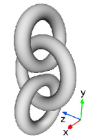
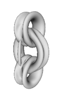
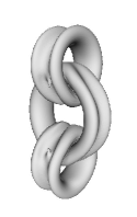
Figure 2: Visualization of the triple ring configuration at $\tau=0$ (left), as well as at $\tau=0.5$ with zero linking number (center) and finite linking number (right). The three images are in the same scale. The change in the direction of the field in the upper ring gives rise to a corresponding change in the value of the magnetic helicity. In the center we can see the emergence of a new flux ring encompassing the two outer rings. Such a ring is not seen on the right.

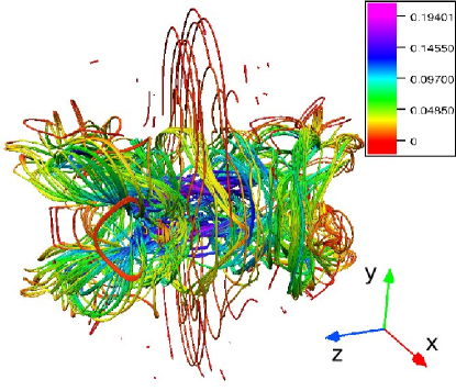
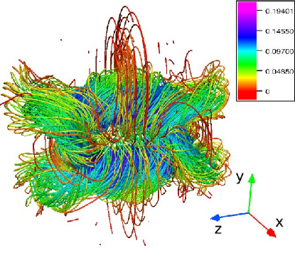
Figure 3: (Color online) Magnetic flux tubes at time $\tau=4$ for the case of zero linking number (upper picture) and finite linking number (lower picture). The colors represent the magnitude of the magnetic field, where the scale goes from red (lowest) over green to blue (highest).

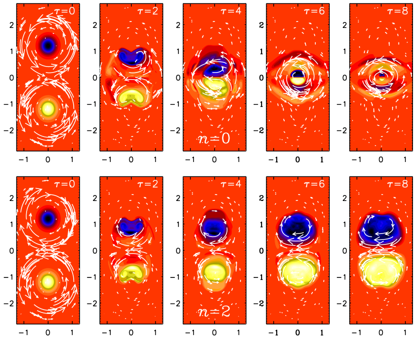
Figure 4: (Color online) Cross-sections in the $xy$ plane of the magnetic field with zero linking number (upper row) and finite linking number (lower row). The $z$ component (pointing out of the plane) is shown together with vectors of the field in the plane. Light (yellow) shades indicate positive values and dark (blue) shades indicate negative values. Intermediate (red) shades indicate zero value.

At early times, visualizations of the field show little difference, but at time $\tau=0.5$ some differences emerge in that the configuration with zero linking number develops an outer ring encompassing the two rings that are connected via the inner ring; see Fig. 2. This outer ring is absent in the configuration with finite linking number.

The change in topology becomes somewhat clearer if we plot the magnetic field lines (see Fig. 3). For the $n=2$ configuration, at time $\tau=4$ one can still see a structure of three interlocked rings, while for the $n=0$ case no clear structure can be recognized. Note that the magnitude of the magnetic field has diminished more strongly for $n=0$ than for $n=2$. This is in accordance with our initial expectations.

The differences between the two configurations become harder to interpret at later times. Therefore we compare in Fig. 4 cross-sections of the magnetic field for the two cases. The $xy$ cross-sections show clearly the development of the new outer ring in the zero linking number configuration. From this figure it is also evident that the zero linking number case suffers more rapid decay because of the now anti-aligned magnetic fields (in the upper panel $B_{x}$ is of opposite sign about the plane $y=0$ while it is negative in the lower panel).

The evolution of magnetic energy is shown in Fig. 5 for the cases with zero and finite linking numbers. Even at the time $\tau\approx 0.6$, when the rings have just come into mutual contact, there is no clear difference in the decay for the two cases. Indeed, until the time $\tau\approx 2$ the magnetic energy evolves still similarly in the two cases, but then there is a pronounced difference where the energy in the zero linking number case shows a rapid decline (approximately like $t^{-3/2}$), while in the case with finite linking number it declines much more slowly (approximately like $t^{-1/3}$). However, power law behavior is only expected under turbulent conditions and not for the relatively structured field configurations considered here. The energy decay in the zero linking number case is roughly the same as in a case of three flux rings that are not interlocked. The result of a corresponding control run is shown as a dotted line in Fig. 5. At intermediate times, $0.5<\tau<5$, the magnetic energy of the control run has diminished somewhat faster than in the interlocked case with $n=0$. It is possible that this is connected with the interlocked nature of the flux rings in one of the cases. Alternatively, this might reflect the presence of rather different dynamics in the non-interlocked case, which seems to be strongly controlled by oscillations on the Alfvén time scale. Nevertheless, at later times the decay laws are roughly the same for non-interlocked and interlocked non-helical cases.

Figure 5: Decay of magnetic energy (normalized to the initial value) for linking numbers 2 (solid line) and 0 (dashed line). The dotted line gives the decay for a control run with non-interlocked rings. The dash-dotted lines indicate $t^{1/3}$ and $t^{3/2}$ scalings for comparison. The inset shows the evolution of the maximum field strength in units of the thermal equipartition value, $B_{\rm th}=c_{\rm s}(\rho_{0}\mu_{0})^{1/2}$.

The time when the rings come into mutual contact is marked by a maximum in the kinetic energy at $\tau\approx 0.6$. This can be seen from Fig. 6, where we compare kinetic and magnetic energies separately for the cases with finite and zero linking numbers. Note also that in the zero-linking number case magnetic and kinetic energies are nearly equal and decay in the same fashion.

Figure 6: Comparison of the evolution of kinetic and magnetic energies in the cases with finite and with vanishing linking numbers. Note that in both cases the maximum kinetic energy is reached at the time $\tau\approx 0.6$. The two cases begin to depart from each other after $\tau\approx 2$. In the non-helical case the magnetic energy shows a sharp drop and reaches equipartition with the kinetic energy, while in the helical case the magnetic energy stays always above the equipartition value.

Next we consider the evolution of magnetic helicity in Fig. 7. Until the time $\tau\approx 0.6$ the value of the magnetic helicity has hardly changed at all. After that time there is a gradual decline, but it is slower than the decline of magnetic energy. Indeed, the ratio $\langle\mathchoice{\mbox{\boldmath$\displaystyle A$}}{\mbox{\boldmath$\textstyle A$}}{\mbox{\boldmath$\scriptstyle A$}}{\mbox{\boldmath$\scriptscriptstyle A$}}{}\cdot\mathchoice{\mbox{\boldmath$\displaystyle B$}}{\mbox{\boldmath$\textstyle B$}}{\mbox{\boldmath$\scriptstyle B$}}{\mbox{\boldmath$\scriptscriptstyle B$}}{}\rangle/\langle\mathchoice{\mbox{\boldmath$\displaystyle B$}}{\mbox{\boldmath$\textstyle B$}}{\mbox{\boldmath$\scriptstyle B$}}{\mbox{\boldmath$\scriptscriptstyle B$}}{}^{2}\rangle$, which corresponds to a length scale, shows a gradual increase from $0.1R_{\rm o}$ to nearly $0.6R_{\rm o}$ at the end of the simulation. This reflects the fact that the field has become smoother and more space-filling with time.

Figure 7: Evolution of magnetic helicity in the case with finite linking number. In the upper panel, $\langle\mathchoice{\mbox{\boldmath$\displaystyle A$}}{\mbox{\boldmath$\textstyle A$}}{\mbox{\boldmath$\scriptstyle A$}}{\mbox{\boldmath$\scriptscriptstyle A$}}{}\cdot\mathchoice{\mbox{\boldmath$\displaystyle B$}}{\mbox{\boldmath$\textstyle B$}}{\mbox{\boldmath$\scriptstyle B$}}{\mbox{\boldmath$\scriptscriptstyle B$}}{}\rangle$ is normalized to its initial value (indicated by subscript 0) while in the lower panel it is normalized to the magnetic energy divided by $R_{\rm o}$.

Given that the magnetic helicity decays only rather slowly, one must expect that the fluxes $\Phi_{i}$ of the three rings also only change very little. Except for simple configurations where flux tubes are embedded in field-free regions, it is in general difficult to measure the actual fluxes, as defined in Eq. (5). On the other hand, especially in observational solar physics, one often uses the so-called unsigned flux Zwa85 ; SH94 , which is defined as

$$P_{\rm 2D}=\int_{S}|\mathchoice{\mbox{\boldmath$\displaystyle B$}}{\mbox{\boldmath$\textstyle B$}}{\mbox{\boldmath$\scriptstyle B$}}{\mbox{\boldmath$\scriptscriptstyle B$}}{}|\,dS.$$ (9)

For a ring of flux $\Phi$ that intersects the surface in the middle at right angles the net flux cancels to zero, but the unsigned flux gets contributions from both intersection, so $P_{\rm 2D}=2|\Phi|$. In three-dimensional simulations it is convenient to determine

$$P=\int_{V}|\mathchoice{\mbox{\boldmath$\displaystyle B$}}{\mbox{\boldmath$\textstyle B$}}{\mbox{\boldmath$\scriptstyle B$}}{\mbox{\boldmath$\scriptscriptstyle B$}}{}|\,dV.$$ (10)

For several rings, all with radius $R$, we have

$$P=2\pi R\sum_{i=1}^{N}|\Phi_{i}|=\pi NRP_{\rm 2D},$$ (11)

where $N$ is the number of rings. In Fig. 8 we compare the evolution of $P$ (normalized to the initial value $P_{0}$) for the cases with $n=0$ and $n=2$. It turns out that after $\tau=1$ the value of $p$ is nearly constant for $n=2$, but not for $n=0$.

Figure 8: Decay of the unsigned magnetic flux $P$ (normalized to the initial value $P_{0}$) for the cases with $n=0$ and $n=2$. The dotted line gives the decay for a control run with non-interlocked rings.

Let us now return to the earlier question of whether a flux configuration with zero linking number can have finite spectral magnetic helicity, i.e. whether $H(k)$ is finite but of opposite sign at different values of $k$. The spectra $M(k)$ and $H(k)$ are shown in Fig. 9 for the two cases at time $\tau=5$. This figure shows that in the configuration with zero linking number $H(k)$ is essentially zero for all values of $k$. This is not the case and, in hindsight, is hardly expected; see Fig. 9 for the spectra of $M(k)$ and $k|H(k)|/2\mu_{0}$ in the two cases at $\tau=5$. What might have been expected is a segregation of helicity not in the wave-number space, but in the physical space for positive and negative values of $y$. It is then possible that magnetic helicity has been destroyed by locally generated magnetic helicity fluxes between the two domains in $y>0$ and $y<0$. However, this is not pursued further in this paper.

Figure 9: Comparison of spectra of magnetic energy and magnetic helicity in the case with zero linking number (upper panel) and finite linking number (lower panel) at $\tau=5$. Stretches with negative values of $H(k)$ are shown as dotted lines.

In order to understand in more detail the way the energy is dissipated, we plot in Fig. 10 the evolution of the time derivative of the magnetic energy $E_{\rm M}={1\over 2\mu_{0}}\int\mathchoice{\mbox{\boldmath$\displaystyle B$}}{\mbox{\boldmath$\textstyle B$}}{\mbox{\boldmath$\scriptstyle B$}}{\mbox{\boldmath$\scriptscriptstyle B$}}{}^{2}\,dV$ (upper panel) and the kinetic energy $E_{\rm K}={\textstyle{1\over 2}}\int\rho\mathchoice{\mbox{\boldmath$\displaystyle U$}}{\mbox{\boldmath$\textstyle U$}}{\mbox{\boldmath$\scriptstyle U$}}{\mbox{\boldmath$\scriptscriptstyle U$}}{}^{2}\,dV$ (lower panel). In the lower panel we also show the rate of work done by the Lorentz force, $W_{\rm L}=\int\mathchoice{\mbox{\boldmath$\displaystyle U$}}{\mbox{\boldmath$\textstyle U$}}{\mbox{\boldmath$\scriptstyle U$}}{\mbox{\boldmath$\scriptscriptstyle U$}}{}\cdot(\mathchoice{\mbox{\boldmath$\displaystyle J$}}{\mbox{\boldmath$\textstyle J$}}{\mbox{\boldmath$\scriptstyle J$}}{\mbox{\boldmath$\scriptscriptstyle J$}}{}\times\mathchoice{\mbox{\boldmath$\displaystyle B$}}{\mbox{\boldmath$\textstyle B$}}{\mbox{\boldmath$\scriptstyle B$}}{\mbox{\boldmath$\scriptscriptstyle B$}}{})\,dV$, and in the upper panel we show the rate of work done against the Lorentz force, $-W_{\rm L}$. All values are normalized by $E_{\rm M0}/T_{\rm s}$, where $E_{\rm M0}$ is the value of $E_{\rm M}$ at $\tau=0$.

The rates of magnetic and kinetic energy dissipation, $\epsilon_{\rm M}$ and $\epsilon_{\rm K}$, respectively, can be read off as the difference between the two curves in each of the two panels in Fig. 10. Indeed, we have

$$-W_{\rm L}-dE_{\rm M}/dt=\epsilon_{\rm M},$$ (12)

$$W_{\rm L}+W_{\rm C}-dE_{\rm K}/dt=\epsilon_{\rm K},$$ (13)

where the compressional work term $W_{\rm C}=\int p\mathchoice{\mbox{\boldmath$\displaystyle\nabla$}}{\mbox{\boldmath$\textstyle\nabla$}}{\mbox{\boldmath$\scriptstyle\nabla$}}{\mbox{\boldmath$\scriptscriptstyle\nabla$}}{}\cdot\mathchoice{\mbox{\boldmath$\displaystyle U$}}{\mbox{\boldmath$\textstyle U$}}{\mbox{\boldmath$\scriptstyle U$}}{\mbox{\boldmath$\scriptscriptstyle U$}}{}\,{\rm d}{}V$ is found to be negligible in all cases. Looking at Fig. 10 we can say that at early times ($0<\tau<0.7$) the magnetic field contributes to driving fluid motions ($W_{\rm L}>0$) while at later times some of the magnetic energy is replenished by kinetic energy ($W_{\rm L}<0$), but since magnetic energy dissipation still dominates, the magnetic energy is still decaying ($dE_{\rm M}/dt<0)$. The maximum dissipation occurs around the time $\tau=0.7$. The magnetic energy dissipation is then about twice as large as the kinetic energy dissipation. We note that the ratio between magnetic and kinetic energy dissipations should also depend on the value of the magnetic Prandtl number, $\mbox{\rm Pr}_{\rm M}=\nu/\eta$, which we have chosen here to be unity. In this connection it may be interesting to recall that one finds similar ratios of $\epsilon_{\rm K}$ and $\epsilon_{\rm M}$ both for helical and non-helical turbulence HBD03 . At smaller values of $\mbox{\rm Pr}_{\rm M}$ the ratio of $\epsilon_{\rm K}$ to $\epsilon_{\rm K}+\epsilon_{\rm M}$ diminishes like $\mbox{\rm Pr}_{\rm M}^{-1/2}$ for helical turbulence B09 . In the present case the difference between $n=0$ and 2 is, again, small. Only at later times there is a small difference in $W_{\rm L}$, as is shown in the inset of Fig. 10. It turns out that, for $n=2$, $W_{\rm L}$ is positive while for $n=0$ its value fluctuates around zero. This suggests that the $n=2$ configuration is able to sustain fluid motions for longer times than the $n=0$ configuration. This is perhaps somewhat unexpected, because the helical configuration ($n=2$) should be more nearly force free than the non-helical configuration. However, this apparent puzzle is simply explained by the fact that the $n=2$ configuration has not yet decayed as much as the $n=0$ configuration has.

Figure 10: Evolution of the rate of work done against the Lorentz force, $-W_{\rm L}$, together with ${\rm d}{}E_{\rm M}/{\rm d}{}t$ (upper panel), as well as the rate of work done by the Lorentz force, $+W_{\rm L}$, together with ${\rm d}{}E_{\rm K}/{\rm d}{}t$ (lower panel), all normalized in units of $E_{\rm M}/T_{\rm s}$, for the case with finite linking number. The inset shows $-W_{\rm L}$ at late times for the case with $n=0$ (solid line) and $n=2$ (dashed line).

IV Conclusions

The present work has shown that the rate of magnetic energy dissipation is strongly constrained by the presence of magnetic helicity and not by the qualitative degree of knottedness. In our example of three interlocked flux rings we considered two flux chains, where the topology is the same except that the relative orientation of the magnetic field is reversed in one case. This means that the linking number switches from 2 to 0, just depending on the sign of the field in one of the rings. The resulting decay rates are dramatically different in the two cases, and the decay is strongly constrained in the case with finite magnetic helicity.

The present investigations reinforce the importance of considering magnetic helicity in studies of reconnection. Reconnection is a subject that was originally considered in two-dimensional studies of X-point reconnection Par57 ; Bis86 . Three-dimensional reconnection was mainly considered in the last 20 years. An important aspect is the production of current sheets in the course of field line braiding Ber93 . Such current sheets are an important contributor to coronal heating GN96 . The crucial role of magnetic helicity has also been recognized in several papers Hu97 ; Liu07 . However, it remained unclear whether the decay of interlocked flux configurations with zero helicity might be affected by the degree of tangledness. Our present work suggests that a significant amount of dissipation should only be expected from tangled magnetic fields that have zero or small magnetic helicity, while tangled regions with finite magnetic helicity should survive longer and are expected to dissipate less efficiently.

- (1) J. B. Taylor, Phys. Rev. Lett. 33, 1139 (1974).
- (2) T. H. Jensen and M. S. Chu, Phys. Fluids 27, 2881 (1984).
- (3) M. Berger and G. B. Field, J. Fluid Mech. 147, 133 (1984).
- (4) D. M. Rust and A. Kumar, Sol. Phys. 155, 69 (1994).
- (5) D. M. Rust and A. Kumar, Astrophys. J. 464, L199 (1996).
- (6) B. C. Low, Sol. Phys. 167, 217 (1996).
- (7) A. Brandenburg, K. Enqvist, and P. Olesen, Phys. Rev. D 54, 1291 (1996).
- (8) G. B. Field and S. M. Carroll, Phys. Rev. D 62, 103008 (2000).
- (9) M. Christensson, M. Hindmarsh, and A. Brandenburg, Astron. Nachr. 326, 393 (2005).
- (10) A. Pouquet, U. Frisch, and J. Léorat, J. Fluid Mech. 77, 321 (1976).
- (11) A. Brandenburg and K. Subramanian, Phys. Rep. 417, 1 (2005).
- (12) L. Woltjer, Proc. Natl. Acad. Sci. U.S.A. 44, 489 (1958).
- (13) H. K. Moffatt, J. Fluid Mech. 35, 117 (1969).
- (14) M. Berger, Geophys. Astrophys. Fluid Dyn. 30, 79 (1984).
- (15) M.-M. Mac Low, R. S. Klessen, and A. Burkert, Phys. Rev. Lett. 80, 2754 (1998).
- (16) D. Biskamp and W.-C. Müller, Phys. Rev. Lett. 83, 2195 (1999).
- (17) E. Priest and T. Forbes, Magnetic Reconnection, Cambridge University Press, 2000
- (18) A. Ruzmaikin and P. Akhmetiev, Phys. Plasmas 1, 331 (1994).
- (19) G. Hornig and C. Mayer, J. Phys. A 35, 3945 (2002).
- (20) R. Komendarczyk, Commun. Math. Phys. 292, 431 (2009).
- (21) R. M. Kerr and A. Brandenburg, Phys. Rev. Lett. 83, 1155 (1999).
- (22) R. Grauer and C. Marliani, Phys. Rev. Lett. 84, 4850 (2000).
- (23) Zwaan, C., Sol. Phys. 100, 397 (1985).
- (24) C. J. Schrijver and K. L. Harvey, Sol. Phys. 150, 1 (1994).
- (25) N. E. L. Haugen, A. Brandenburg, and W. Dobler, Astrophys. J. 597, L141 (2003).
- (26) A. Brandenburg, Astrophys. J. 697, 1206 (2009).
- (27) E. N. Parker, J. Geophys. Res. 62, 509 (1957).
- (28) D. Biskamp, Phys. Fluids 29, 1520 (1986).
- (29) M. A. Berger, Phys. Rev. Lett. 70, 705 (1993).
- (30) K. Galsgaard and Å. Nordlund, J. Geophys. Res. 101, 13445 (1996).
- (31) Y. Q. Hu, L. D. Xia, X. Li, J. X. Wang, and G. X. Ai, Sol. Phys. 170, 283 (1997).
- (32) Y. Liu, H. Kurokawa, C. Liu, D. H. Brooks, J. Dun, T. T. Ishii, and H. Zhang, Sol. Phys. 240, 253 (2007).