Searching a bitstream in linear time
for the longest substring of any given density

Abstract

Given an arbitrary bitstream, we consider the problem of finding the longest substring whose ratio of ones to zeroes equals a given value. The central result of this paper is an algorithm that solves this problem in linear time. The method involves (i) reformulating the problem as a constrained walk through a sparse matrix, and then (ii) developing a data structure for this sparse matrix that allows us to perform each step of the walk in amortised constant time. We also give a linear time algorithm to find the longest substring whose ratio of ones to zeroes is bounded below by a given value. Both problems have practical relevance to cryptography and bioinformatics.

1 Introduction

Consider a bitstream of length $n$, that is, a sequence of bits $x_{1},x_{2},\ldots,x_{n}$ where each $x_{i}$ is $0$ or $1$. We define the density of this bitstream to be the proportion of bits that are equal to one (equivalently, $\sum x_{i}/n$). The density always lies in the range $[0,1]$: a stream of zeroes has density $0$, a stream of ones has density $1$, and a stream of random bits should have density close to $\frac{1}{2}$.

In this paper we are interested in the densities of substrings within a bitstream. By a substring, we mean a continuous sequence of bits $x_{a},x_{a+1},\ldots,x_{b-1},x_{b}$, beginning at some arbitrary position $a$ and ending at some arbitrary position $b$. The length of a substring is the number of bits that it contains (that is, $b-a+1$), and the density of the substring is likewise the proportion of ones that it contains (that is, $\sum_{i=a}^{b}x_{i}/(b-a+1)$).

In particular, we are interested in the following two problems:

Problem 1.1 (Fixed density problem).

Suppose we are given a bitstream $S$ of length $n$ and a fixed ratio $\theta\in[0,1]$. What is the longest substring of $S$ whose density is equal to $\theta$?

Problem 1.2 (Bounded density problem).

Suppose we are given a bitstream $S$ of length $n$ and a fixed ratio $\theta\in[0,1]$. What is the longest substring of $S$ whose density is at least $\theta$?

For example, suppose we are given the bitstream $S=010110101100$ of length $n=12$. Then the longest substring with density equal to $\theta=0.6$ has length ten ($0\underline{\mathbf{1011010110}}0$), and the longest substring with density at least $\theta=0.7$ has length seven ($010\underline{\mathbf{1101011}}00$). Note that each problem might have many solutions or no solution at all.

Both of these problems have important applications for cryptography. Many cryptographic systems are dependent on pseudo-random number generators (PRNGs), and any unwanted predictability or structure in a PRNG becomes a potential attack point for the underlying cryptosystem. For this reason PRNGs are typically subjected to a stringent series of randomness tests, such as those described in [13] or [15].

Boztaş et al. have recently designed a new series of randomness tests based on the densities of substrings [3]. To construct these tests, they use the Erdős-Rényi law of large numbers [1, 7] to compute the limiting distributions for solutions to the fixed density problem, the bounded density problem and related problems. They then compare observed values against these limiting distributions, and they have identified a possible weakness in the Dragon stream cipher [4] as a result.

Locating substrings with various density properties also has important applications in bioinformatics. A sequence of DNA consists of a long string of nucleotides marked G, C, T or A, and subsequences with high proportions of G and C are called GC-rich regions. GC-richness is correlated with factors such as gene density [18], gene length [6], recombination rates [8], codon usage [17], and the increasing complexity of organisms [2, 11].

To identify GC-rich regions we convert a DNA sequence into a bitstream, where each G or C becomes a one bit, and each T or A becomes a zero bit. We then search for high-density substrings in this bitstream, using techniques such as those discussed here.

Further applications of density problems in the field of bioinformatics are discussed by Goldwasser et al. [9] and Lin et al. [14]. In addition, Greenberg [10] signals potential applications in the field of image processing.

The focus of this paper is on finding fast algorithms to solve Problems 1.1 and 1.2. Both problems allow simple brute-force algorithms that run in $O(n^{2})$ time. For the fixed density problem, Boztaş et al. improve on this with their SkipMisMatch algorithm [3], which remains $O(n^{2})$ in the worst case but has an improved average-case time complexity of $O(n\log n)$. We outline their contribution in Section 2.

Our first contribution in this paper is a series of simple algorithms that solve both the fixed and bounded density problems in $O(n\log n)$ time, even in the worst case. These algorithms are easy to implement and effective in practice, and are based upon a central geometric observation. We cover these log-linear algorithms in Section 3.

In Section 4 we follow with our main result, which is an algorithm that solves the fixed density problem in $O(n)$ time, again in the worst case. Based on one of the previous log-linear algorithms, this algorithm introduces a specialised data structure that allows us to process each bit of the bitstream in amortised constant time. Broadly speaking, we:

• express our bitstream as a sequence of steps through a sparse matrix, where each step requires a localised search and possible insertion into this matrix;

• design a specialised data structure that “compresses” this sparse matrix, so that each localised search and insertion can be performed in amortised constant time.

The amortised analysis is based on aggregation—in essence we count the “interesting” steps of the algorithm by associating them with distinct elements of the bitstream, thereby showing the number of such steps to be $O(n)$. Details of the proof are given in Section 4.3.

Our final contribution is in Section 5, where we give an $O(n)$ time algorithm for the bounded density problem. In contrast to the fixed density problem, this final algorithm is quite simple, involving just a handful of linear scans.

To conclude, we measure the practical performance of our algorithms in Section 6. It is reassuring to find that our linear algorithms are worth the extra difficulty, consistently outperforming the other algorithms for large bitstream lengths $n$.

In related work, several authors have considered problems of finding maximal density substrings in a bitstream subject to a variety of constraints. See in particular work by Lin et al. [14], who place a lower bound on the length of the substring; Goldwasser et al. [9], who improve the prior solution and also place both lower and upper bounds; and Greenberg [10], who studies a variant relating to compressed bitstreams.

Hsieh et al. [12] study a series of more general problems, where the bitstream is replaced by a sequence of real numbers, and the density of a substring becomes the average of the corresponding subsequence. In addition to developing algorithms, they show that several such problems—including the fixed density problem—have a lower bound of $\Omega(n\log n)$ time. Our linear algorithm effectively breaks through this lower bound in the case where the input sequence consists entirely of zeroes and ones.

Throughout this paper we measure time complexity in “number of operations”, where we treat basic arithmetical operations such as $+$ and $\times$ as constant-time.

2 Quadratic Algorithms: Boztaş et al.

In this section we outline the prior work of Boztaş et al., including a simple $O(n^{2})$ brute force algorithm as well as their SkipMisMatch algorithm, which remains $O(n^{2})$ in the worst case but becomes $O(n\log n)$ in the average case.

Assumption 2.1.

Throughout this paper we assume that the ratio $\theta$ is given as a rational $\theta=\alpha/\beta$, where $\alpha$ and $\beta$ are integers in the range $0\leq\alpha\leq\beta\leq n$, and where $\gcd(\alpha,\beta)=1$.

This assumption is not restrictive in any way. If $\theta$ cannot be expressed as above then the fixed density problem has no solution, and for the bounded density problem we can harmlessly replace $\theta$ with a nearby rational that satisfies our requirements.

A naïve brute force solution runs in $O(n^{3})$ time: for each possible start point and end point, walk through the substring and count the ones. However, there are several different tricks that can easily convert this into $O(n^{2})$ by replacing “walk through the substring” with a constant time operation. One such trick is to use a rank table.

Definition 2.2 (Rank Table).

A rank table is an array $r_{0},r_{1},\ldots,r_{n}$, where each entry $r_{k}$ counts the number of ones in the substring $x_{1},\ldots,x_{k}$.

In other words, $r_{k}=\sum_{i=1}^{k}x_{i}$. It is clear that the complete rank table can be precomputed in $O(n)$ time, and that it supports constant time queries of the form “how many ones appear in the substring $x_{a},\ldots,x_{b}$?” by simply computing $r_{b}-r_{a-1}$.

For the fixed density problem, the SkipMisMatch algorithm further optimises this $O(n^{2})$ brute force method by making the following observations:

1. We are searching for the longest substring of density $\theta$. We can therefore reorganise our search to work from the longest substring down to the shortest, allowing us to terminate as soon as we find any substring of density $\theta$.

2. If we find such a substring, its length must be a multiple of $\beta$ (where $\theta=\alpha/\beta$ as above). We can therefore restrict our search to substrings of such lengths.

3. When searching for substrings of length $k\beta$, we need to find precisely $k\alpha$ ones to give a density of $\theta$. If at some point we find $k\alpha\pm\epsilon$ ones, we must step forward at least $\epsilon$ positions in our bitstream before we can “undo the error” and potentially find the $k\alpha$ ones that we seek.

procedure SkipMisMatch($x_{1},\ldots,x_{n},\ \theta=\alpha/\beta$)     Build a rank table $r_{0},r_{1},\ldots,r_{n}$     for $k\leftarrow\lfloor\frac{n}{\beta}\rfloor$ downto $1$ do $\triangleright$ Search for substrings of length $k\beta$          $(a,b)\leftarrow(1,k\beta)$ $\triangleright$ Initial start and end for our substring          while $b\leq n$ do              $\epsilon\leftarrow|k\alpha-(r_{b}-r_{a-1})|$ $\triangleright$ Compute the “error” for this substring              if $\epsilon=0$ then                  Output $(a,b)$ and terminate              else                  $(a,b)\leftarrow(a+\epsilon,b+\epsilon)$ $\triangleright$ We can safely skip forward $\epsilon$ positions                                Output “no such substring” and terminate

Figure 1: The SkipMisMatch algorithm for the fixed density problem

Bundling these observations together, we obtain the SkipMisMatch algorithm as illustrated in Figure 1. The worst-case complexity is clearly still $O(n^{2})$, but for a random bitstream the expected performance can be significantly better. In particular, Boztaş et al. prove the following result as a part of [3, Lemma 4]:

Lemma 2.3.

Suppose we have a random bitstream, where each bit is one with probability $\rho$ or zero with probability $1-\rho$. Then SkipMisMatch has expected time bounded by

$$O\left(|\theta-\rho|^{-1}\times\frac{n}{\beta}\log\frac{n}{\beta}\right).$$

For fixed $\theta$ and $\rho$, this reduces to an expected time of $O(n\log n)$, as long as $\theta\neq\rho$. However, if we retain the dependency on $\theta$ (and hence its denominator $\beta$), we find that SkipMisMatch is rewarded by large denominators $\beta$ (which enhance the power of optimisation (ii)), and is penalised by values of $\theta$ close to $\rho$ (which limit the use of optimisation (iii)).

To summarise, the SkipMisMatch algorithm is easy to code and runs significantly faster than brute force, but its performance depends heavily on the given value of $\theta$. In addition, some broader issues might arise—the expected $O(n\log n)$ time is appropriate for random bitstreams (as found in cryptographic applications, for instance), but might not hold for applications such as bioinformatics and image processing where bitstreams become more structured. Moreover, the algorithm does not translate well to the bounded density problem. All of these reasons highlight the need for faster and more robust algorithms, which form the subject of the remainder of this paper.

3 Log-Linear Algorithms: Maps and Sorting

In this section we introduce our first truly sub-quadratic algorithms for solving the fixed and bounded density problems. We describe DistMap, a simple algorithm involving a map structure, and DistSort, a variation that replaces this map with a sort and a linear scan. Both of these algorithms run in $O(n\log n)$ time, even in the worst case.

Although we present even faster algorithms in Sections 4 and 5, both DistMap and DistSort are simple to describe and easy to implement. Moreover, both algorithms play important roles: DistMap is the foundation upon which the linear algorithm of Section 4 is built, and DistSort is a more flexible variant that can solve both the fixed and bounded density problems.

3.1 Graphical Representations

Our first step in developing these sub-quadratic algorithms is to find a graphical representation for our bitstreams.

Definition 3.1 (Grid Representation).

We can plot any bitstream as a walk through an infinite two-dimensional grid as follows. We begin at the origin $(0,0)$, and then step one unit in the $x$-direction each time we encounter a zero, or one unit in the $y$-direction each time we encounter a one, as illustrated in Figure 2. We refer to this as the grid representation of the bitstream.

Figure 2: The grid representation for the bitstream $010110101100$

All of the new algorithms developed in this paper are based upon the following simple geometric observation:

Lemma 3.2.

A substring of a bitstream has density $\theta$ if and only if the line joining its start and end points in the grid representation has gradient $\frac{\theta}{1-\theta}$.

To illustrate, Figure 3 builds on the previous example by searching for substrings of density $\theta=0.6$. Several pairs of points separated by gradient $\frac{\theta}{1-\theta}=1.5$ are marked (though there are several more such pairs that are not marked). The first two pairs correspond to substrings of length five, and the third pair corresponds to a substring of length ten.

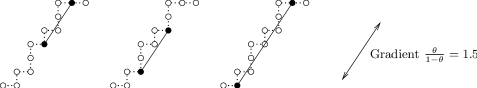
Figure 3: Pairs of points that represent substrings of density $\theta=0.6$

We can find such pairs of points by drawing a line $L_{\theta}$ through the origin with slope $\frac{\theta}{1-\theta}$, and then measuring the distance of each point from this line (where distances are signed, so that points above or below the line have positive or negative distance respectively). This is illustrated in Figure 4. It is clear that two points are joined by a line of gradient $\frac{\theta}{1-\theta}$ if and only if their distances from $L_{\theta}$ are the same.

Figure 4: Measuring the distance of each point from the line $L_{\theta}$

Although such distances can be messy to compute, with appropriate rescaling we can convert them into integers as follows.

Definition 3.3 (Distance Sequence).

Recall from Assumption 2.1 that $\theta=\alpha/\beta$, where $\gcd(\alpha,\beta)=1$. For a given bitstream $x_{1},\ldots,x_{n}$, we define the distance sequence $d_{0},d_{1},\ldots,d_{n}$ by the formula

$$d_{i}=(\beta-\alpha)\cdot(\mbox{number of ones in $x_{1},\ldots,x_{i}$})-\alpha\cdot(\mbox{number of zeroes in $x_{1},\ldots,x_{i}$}).$$

In other words, $d_{i}=(\beta-\alpha)r_{i}-\alpha(i-r_{i})=\beta r_{i}-\alpha i$, where $r_{i}$ is the corresponding entry in the rank table.

With a little thought it can be seen that $d_{i}$ is proportional to the distance from $L_{\theta}$ of the point at the end of the $i$th step of the walk. This empowers the distance sequence with the following critical property:

Lemma 3.4.

The substring $x_{a},\ldots,x_{b}$ has density equal to $\theta$ if and only if $d_{a-1}=d_{b}$. Similarly, the substring $x_{a},\ldots,x_{b}$ has density at least $\theta$ if and only if $d_{a-1}\leq d_{b}$.

Proof.

Although this follows immediately from the geometric argument above, we can also prove it directly. Using the formula $d_{i}=\beta r_{i}-\alpha i$, we find that $d_{a-1}=d_{b}$ if and only if $\beta(r_{b}-r_{a-1})=\alpha(b-a+1)$, or equivalently

$$\mbox{density of $x_{a},\ldots,x_{b}$}=\frac{r_{b}-r_{a-1}}{b-a+1}=\frac{\alpha}{\beta}=\theta.$$

The argument for density $\geq\theta$ is similar. ∎

3.2 The DistMap Algorithm

With Lemma 3.4 we now have a simple solution to the fixed density problem. We compute the distance sequence $d_{0},\ldots,d_{n}$ as we pass through our bitstream, keeping track of which distances we have seen before and when we first saw them. Whenever we find that a distance has been seen before, we have a substring of density $\theta$ and therefore a potential solution.

We keep track of previously-seen distances using a $\mathit{key}\mapsto\mathit{value}$ map structure with worst-case $O(\log n)$ search and insertion, such as a red-black tree [5]. Here the key is a distance $D$ that we have seen before, and the value is the position at which we first saw it (i.e., the smallest $i$ for which $d_{i}=D$).

procedure DistMap($x_{1},\ldots,x_{n},\ \theta=\alpha/\beta$)     $(a,b)\leftarrow(0,0)$ $\triangleright$ Best start/end found so far     $\delta\leftarrow 0$ $\triangleright$ Current distance $d_{i}$     Initialise the empty map $m$     Insert $m[0]\leftarrow 0$ $\triangleright$ Record the starting point $d_{0}=0$     for $i\leftarrow 1$ to $n$ do          if $x_{i}=1$ then $\triangleright$ Compute the new distance $d_{i}$              $\delta\leftarrow\delta+(\beta-\alpha)$          else              $\delta\leftarrow\delta-\alpha$                    if $m$ has no key $\delta$ then $\triangleright$ Have we seen this distance before?              Insert $m[\delta]\leftarrow i$ $\triangleright$ No, this is the first time          else              if $i-m[\delta]>b-a+1$ then $\triangleright$ Yes, back at position $m[\delta]$                  $(a,b)\leftarrow(m[\delta]+1,i)$ $\triangleright$ Longest substring found so far                                Output $(a,b)$

Figure 5: The DistMap algorithm for the fixed density problem

The result is the algorithm DistMap, described in Figure 5. Given our choice of map structure, the following result is clear:

Lemma 3.5.

The algorithm DistMap solves the fixed density problem in $O(n\log n)$ time in the worst case.

We could of course use a hash table instead of a map structure—with a judicious choice of hash function this could yield $O(n)$ expected time, though the worst case could potentially be much slower. Because we offer a worst-case $O(n)$ algorithm in Section 4, we do not pursue hashing any further here.

3.3 The DistSort Algorithm

We move now to a variant of DistMap that removes any need for a map structure at all. Instead, we replace this map with a simple array that we sort in-place after all $n$ bits of the bitstream have been processed. The new algorithm is named DistSort, and has the following advantages:

• Whilst the map structure plays a key role in giving us $O(n\log n)$ running time, it also comes with a non-trivial memory overhead. If $n$ is large and memory becomes a problem, the in-place sort used by DistSort may be a more economical choice.

• DistMap relies on searching for precise matches $d_{a-1}=d_{b}$ within the map structure. This makes it unsuitable for the bounded density problem, which requires only $d_{a-1}\leq d_{b}$ (Lemma 3.4). If we replace our map with an array sorted by distance $d_{i}$, then both problems become easy to solve. Indeed, we find with DistSort that the solutions for the fixed and bounded density problems differ by just one line.

The key ideas behind DistSort are as follows:

• We walk through the bitstream and compute each distance $d_{i}$ as we go, just as we did for DistMap. However, instead of storing distances in a map, we store each pair $(d_{i},i)$ in a simple array $z[0..n]$, so that each array entry $z[i]$ is the pair $(d_{i},i)$.

• Once we have finished our walk through the bitstream, we sort the array $z[0..n]$ by distance. This gives us a sequence of $(\mathrm{distance},\,\mathrm{position})$ pairs

  $$(D_{0},P_{0})\quad(D_{1},P_{1})\quad\ldots\quad(D_{n},P_{n}),$$

  where $D_{0}\leq D_{1}\leq\ldots\leq D_{n}$ and where each $D_{i}$ is the distance after the $P_{i}$th step.

• Finding positions with matching distances is now a simple matter of walking through the array from left to right—all of the positions with the same distance will be clumped together. In each clump we track the smallest and largest positions ${p_{\mathrm{min}}}$ and ${p_{\mathrm{max}}}$, and these become a candidate substring $x_{({p_{\mathrm{min}}}+1)},\ldots,x_{p_{\mathrm{max}}}$ with density $\theta$. The longest such substring is then our solution to the fixed density problem.

• Solving the bounded density problem is just as easy. The only difference is that we now need our substring $x_{({p_{\mathrm{min}}}+1)},\ldots,x_{p_{\mathrm{max}}}$ to satisfy $d_{p_{\mathrm{min}}}\leq d_{p_{\mathrm{max}}}$, not $d_{p_{\mathrm{min}}}=d_{p_{\mathrm{max}}}$. To achieve this, we simply change ${p_{\mathrm{min}}}$ from the smallest position in this clump to the smallest position in all clumps seen so far.

procedure DistSort($x_{1},\ldots,x_{n},\ \theta=\alpha/\beta$)     Initialise an array $z[0..n]$ of $(\mbox{dist},\mbox{pos})$ pairs     $\delta\leftarrow 0$ $\triangleright$ Current distance $d_{i}$     $z[0]\leftarrow(0,0)$ $\triangleright$ Record the starting point $d_{0}=0$     for $i\leftarrow 1$ to $n$ do          if $x_{i}=1$ then $\triangleright$ Compute the new distance $d_{i}$              $\delta\leftarrow\delta+(\beta-\alpha)$          else              $\delta\leftarrow\delta-\alpha$                    $z[i]\leftarrow(\delta,i)$ $\triangleright$ Store the pair $(d_{i},i)$ in our array          Sort $z[0..n]$ by distance, giving a sorted sequence           of pairs $(D_{0},P_{0})\;(D_{1},P_{1})\;\ldots\;(D_{n},P_{n})$     $(a,b)\leftarrow(0,0)$ $\triangleright$ Best start/end positions found so far     $({p_{\mathrm{min}}},{p_{\mathrm{max}}})\leftarrow(P_{0},P_{0})$ $\triangleright$ Potential start/end positions     $i\leftarrow 0$     while $i\leq n$ do          ${p_{\mathrm{min}}}\leftarrow P_{i}$ $\triangleright$ Do this for the fixed density problem ONLY          ${p_{\mathrm{max}}}\leftarrow P_{i}$          $i\leftarrow i+1$ $\triangleright$ Run through a clump of pairs with the same distance          while $i\leq n$ and $D_{i}=D_{i-1}$ do              if $P_{i}<{p_{\mathrm{min}}}$ then                  ${p_{\mathrm{min}}}\leftarrow P_{i}$ $\triangleright$ A smaller position with this distance                            if $P_{i}>{p_{\mathrm{max}}}$ then                  ${p_{\mathrm{max}}}\leftarrow P_{i}$ $\triangleright$ A larger position with this distance                            $i\leftarrow i+1$                    if ${p_{\mathrm{max}}}-{p_{\mathrm{min}}}>b-a+1$ then              $(a,b)\leftarrow({p_{\mathrm{min}}}+1,{p_{\mathrm{max}}})$ $\triangleright$ Longest substring found so far                   Output $(a,b)$

Figure 6: The DistSort algorithm for the fixed and bounded density problems

The full algorithm is given in Figure 6. The fixed and bounded density algorithms differ by only one line (marked with a comment in bold), where in the bounded case we do not reset ${p_{\mathrm{min}}}$ upon entering a new clump of pairs with equal distances.

Regarding time complexity, we can choose a worst-case $O(n\log n)$ sorting algorithm, such as the introsort algorithm of Musser [16]. The subsequent scan through the array runs in linear time, yielding the following overall result:

Lemma 3.6.

The algorithm DistSort solves both the fixed and bounded density problems in $O(n\log n)$ time in the worst case.

4 Solving the Fixed Density Problem

We proceed now to an algorithm for the fixed density problem that runs in $O(n)$ time, even in the worst case. This algorithm uses DistMap as a starting point, but replaces the generic map structure with a specialised data structure for the task at hand.

The central observation is the following. As we run the DistMap algorithm, each successive key in our map is always obtained by adding $+(\beta-\alpha)$ or $-\alpha$ to the previous key. We exploit this constraint to design a data structure that allows us to “jump” from one key to the next without requiring a full search, thereby eliminating the $\log n$ factor from our running time.

The data structure is fairly detailed, making it difficult to give a simple overview. The following outline summarises the broad ideas involved, but for a clearer picture the reader is referred to the full description in Sections 4.1 and 4.2. The running time of $O(n)$ is established in Section 4.3 using amortised analysis.

• We begin by arranging the integers into an infinite two-dimensional lattice (Figure 7), so that $+(\beta-\alpha)$ represents a single step to the right and $-\alpha$ represents a single step down. This makes moving from one key to the next a local movement within the lattice. This lattice has infinitely many columns but only $\beta-\alpha$ rows, so a step down from the bottom row wraps back around to the top (but with a shift).

  

  Figure 7: The two-dimensional lattice of integers for $\beta-\alpha=3$ and $\alpha=5$.

• We now use this integer lattice as the “domain” of our map, so that keys (the distances $d_{i}$) become points in the lattice, and values (the corresponding positions $i$) are stored at these points. In this way our data structure becomes a matrix, which is sparse because only $n$ points in the lattice correspond to “real” keys with non-empty values.

• The next stage in our design is to “compress” this sparse matrix by storing not individual $\mathit{key}\mapsto\mathit{value}$ pairs but rather horizontal runs of consecutive pairs, as illustrated in Figure 8. Storing just the start and end of each run allows us to completely reconstruct the missing keys and values in between.

  

  $\mathbf{\Longleftrightarrow}$   

  Figure 8: Compressing a horizontal run of consecutive pairs

• We finish by developing a linked structure for storing our matrix. The compressed runs in each row are stored as a “horizontal” linked list, with additional “vertical” links between rows for downward steps. We also chain vertical links together, yielding a perfect balance that offers enough information to support fast movement between keys, but enough flexibility to support fast insertion of new $\mathit{key}\mapsto\mathit{value}$ pairs.

Before presenting the details, it becomes useful to strengthen our base assumptions as follows.

Assumption 4.1.

Recall from Assumption 2.1 that $\theta=\alpha/\beta$, where $0\leq\alpha\leq\beta\leq n$. From here onwards we strengthen this by assuming the stricter bounds $0<\alpha<\beta\leq n$. In other words, we explicitly disallow the special cases $\theta=0$ and $\theta=1$.

Like our earlier assumptions, this is not restrictive in any way. If $\theta=0$ or $\theta=1$ then we simply require the longest continuous substring of zeroes or ones, which is trivial to find in linear time.

4.1 The Mapping Matrix

We begin the details with a formal definition of the integer lattice depicted in Figure 7. Recall from Assumptions 2.1 and 4.1 that both $\beta-\alpha$ and $\alpha$ are strictly positive, and that $\gcd(\beta-\alpha,\alpha)=1$.

Definition 4.2 (Lattice Coordinates).

Let $z$ be any integer. The lattice coordinates of $z$ are the unique solutions $(r,c)$ to the equation

$$(\beta-\alpha)c-\alpha r=z,$$ (1)

for which $r$ and $c$ are integers and $0\leq r<\beta-\alpha$. We call $r$ and $c$ the row and column of $z$ respectively.

For example, consider Figure 7 in which $\beta-\alpha=3$ and $\alpha=5$. The following table lists the lattice coordinates of several integers $z$:

$$\begin{array}[]{l|c|c|c|c|c|c}\mbox{Integer $z$}&-3&0&3&6&1&-4\\ \hline\cr\mbox{Lattice coordinates of $z$}&(0,-1)&(0,0)&(0,1)&(0,2)&(1,2)&(2,2)\end{array}$$

These are precisely the locations at which each integer can be found in Figure 7, where we number the rows and columns so that the integer zero appears at coordinates $(0,0)$.

With a little modular arithmetic it can shown that every integer appears once and only once in our lattice, as expressed formally by the following result. The proof is elementary, and we do not repeat it here.

Lemma 4.3.

Lattice coordinates are always well-defined, that is, equation (1) has a unique solution for every integer $z$. Moreover, every pair of integers $(r,c)$ with $0\leq r<\beta-\alpha$ forms the lattice coordinates of one and only one integer.

It is worth reiterating a key feature of this construction, which is that each bit of the bitstream gives rise to a local movement within the lattice:

Lemma 4.4.

Consider some position $i$ within the bitstream, where $0\leq i<n$. Suppose that the lattice coordinates of the distance $d_{i}$ are $(r,c)$. Then:

• If the $(i+1)$th bit is a one, the lattice coordinates of the subsequent distance $d_{i+1}$ are $(r,c+1)$. That is, we take one step to the right.

• If the $(i+1)$th bit is a zero and $r<\beta-\alpha-1$, then the lattice coordinates of $d_{i+1}$ are $(r+1,c)$. That is, we take one step down.

• If the $(i+1)$th bit is a zero and $r=\beta-\alpha-1$ (i.e., we are on the bottom row of the lattice), then the lattice coordinates of $d_{i+1}$ are $(0,c-\alpha)$. That is, we wrap back around to the top with a shift of $\alpha$ columns to the left.

This is a straightforward consequence of Definitions 3.3 and 4.2, and again we omit the proof. The various movements described in this result are indicated by the solid lines in Figure 7.

Recall that our overall strategy is to build a replacement data structure for the generic $\mathit{key}\mapsto\mathit{value}$ map, whose keys are distances $d_{i}$ and whose values are the corresponding positions $i$ in the bitstream. Using Lemma 4.3 we can replace each distance $d_{i}$ with its lattice coordinates $(r,c)$, thereby replacing the old mapping $d_{i}\mapsto i$ with the new mapping $(r,c)\mapsto i$. This effectively gives us a matrix with $\beta-\alpha$ rows and infinitely many columns, which we formalise as follows.

Definition 4.5 (Mapping Matrix).

We define the mapping matrix to be an infinite matrix with precisely $\beta-\alpha$ rows (numbered $0,\ldots,\beta-\alpha-1$) and infinitely many columns in both directions (numbered $\ldots,-1,0,1,\ldots$). Each cell of this matrix may contain an integer, or may contain the symbol $\varnothing$ representing an empty cell. The entry in row $r$ and column $c$ of the mapping matrix $M$ is denoted ${M}[\,r,\,c\,]$.

Our algorithm now runs as follows. As we process each bit of the bitstream, we walk through the cells of the mapping matrix as described by Lemma 4.4. If we step into an empty cell, we store the current position in the bitstream. If we step into a previously-occupied cell then we have found a substring of density $\theta$.

procedure DistMatrix($x_{1},\ldots,x_{n},\ \theta=\alpha/\beta$)     $(a,b)\leftarrow(0,0)$ $\triangleright$ Best start/end found so far     $(r,c)\leftarrow(0,0)$ $\triangleright$ Current location in the matrix     Initialise the empty mapping matrix $M$     Insert ${M}[\,0,\,0\,]\leftarrow 0$ $\triangleright$ Record the starting point $d_{0}=0$     for $i\leftarrow 1$ to $n$ do          if $x_{i}=1$ then              $c\leftarrow c+1$ $\triangleright$ Step right          else if $r<\beta-\alpha-1$ then              $r\leftarrow r+1$ $\triangleright$ Step down          else              $(r,c)\leftarrow(0,c-\alpha)$ $\triangleright$ Step down and wrap around                    if ${M}[\,r,\,c\,]=\varnothing$ then $\triangleright$ Have we been here before?              Insert ${M}[\,r,\,c\,]\leftarrow i$ $\triangleright$ No, this is the first time          else              if $i-{M}[\,r,\,c\,]>b-a+1$ then $\triangleright$ Yes, back at position ${M}[\,r,\,c\,]$                  $(a,b)\leftarrow({M}[\,r,\,c\,]+1,i)$ $\triangleright$ Longest substring found so far                                Output $(a,b)$

Figure 9: The DistMatrix algorithm for the fixed density problem

The full pseudocode is given in Figure 9, under the algorithm name DistMatrix. The algorithm is of course remarkably similar to DistMap (Figure 5), since the key difference is in the underlying data structure. Our focus in Section 4.2 is now to fully describe this data structure, and thereby describe the critical tasks of evaluating and setting the matrix entry ${M}[\,r,\,c\,]$.

4.2 The Data Structure

We cannot afford to store the mapping matrix as a two-dimensional array, because—even ignoring the infinitely many columns—there are $O(n^{2})$ potential cells that a bitstream of length $n$ might reach. However, only $n+1$ cells are visited (and hence non-empty) for any particular input bitstream. That is, the mapping matrix is sparse.

We therefore aim for a linked structure, where only the cells we visit are stored in memory, and where these cells include pointers to nearby cells to assist with navigation around the matrix.

However, before describing this linked structure we introduce a form of compression, where we only need to store the cells involved in downward steps. As we will see in Section 4.3, this compression is critical for stepping through the matrix in amortised constant time.

Our compression relies on the observation that a run of $k$ consecutive steps to the right produces a sequence of $k$ consecutive values in the matrix:

$$\begin{array}[]{c|c|c|c|c|c}\cline{1-6}\cr{}\hfil&i&i+1&\cdots&i+k&{}\hfil\\ \cline{1-6}\cr\end{array}$$

We can describe such a sequence by storing only the start and end points, without having to store each individual cell in between.

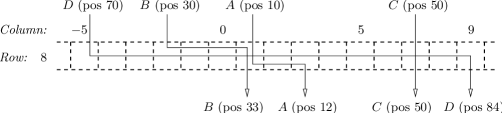
(a) Several paths that cross through a single matrix row

$\begin{array}[]{l@{\quad}c|c|c|c|c|c|c|c|c|c|c|c|c|c|c|c|c}\textit{Column:}&\lx@intercol{}\hfil\hfil\lx@intercol&\lx@intercol\hfil-5\hfil\lx@intercol&\lx@intercol{}\hfil\hfil\lx@intercol&\lx@intercol\hfil 0\hfil\lx@intercol&\lx@intercol{}\hfil\hfil\lx@intercol&\lx@intercol\hfil 5\hfil\lx@intercol&\lx@intercol{}\hfil\hfil\lx@intercol&\lx@intercol\hfil 9\hfil\lx@intercol\\ \lx@intercol{}\hfil\hfil\lx@intercol&\lx@intercol\hfil\mbox{\Large$\downarrow$}\hfil\lx@intercol&\lx@intercol{}\hfil\hfil\lx@intercol&\lx@intercol\hfil\mbox{\Large$\downarrow$}\hfil\lx@intercol&\lx@intercol{}\hfil\hfil\lx@intercol&\lx@intercol\hfil\mbox{\Large$\downarrow$}\hfil\lx@intercol&\lx@intercol{}\hfil\hfil\lx@intercol&\lx@intercol\hfil\mbox{\Large$\downarrow$}\hfil\lx@intercol\\ \cline{2-18}\cr\textit{Row:}\quad 8&{}\hfil&70&71&72&30&31&32&10&11&12&79&80&81&50&83&84&{}\hfil\\ \cline{2-18}\cr\lx@intercol{}\hfil\hfil\lx@intercol&\lx@intercol\hfil\mbox{\Large$\downarrow$}\hfil\lx@intercol&\lx@intercol{}\hfil\hfil\lx@intercol&\lx@intercol\hfil\mbox{\Large$\downarrow$}\hfil\lx@intercol&\lx@intercol{}\hfil\hfil\lx@intercol&\lx@intercol\hfil\mbox{\Large$\downarrow$}\hfil\lx@intercol&\lx@intercol{}\hfil\hfil\lx@intercol&\lx@intercol\hfil\mbox{\Large$\downarrow$}\hfil\lx@intercol\end{array}$

(b) The corresponding values in the mapping matrix

Cell	Value in this cell	Value to start this run
$(8,-5)$	70	70
$(8,-2)$	30	30
$(8,1)$	10	10
$(8,3)$	12	78
$(8,7)$	50	82
$(8,9)$	84	$\varnothing$

(c) Storing these values in memory

Figure 10: Compressing a row of the mapping matrix

This pattern becomes more complicated when new paths through the matrix cross over old paths, but the core idea remains the same—we look for horizontal runs of consecutive values in the matrix, and record only where they start and end. Figure 10 gives an example, where four different paths from four different sections of the bitstream cross through the same row of the matrix.

• Figure 10(a) shows the four paths, which are labelled $A$, $B$, $C$ and $D$ in chronological order as they appear in the bitstream. For instance, path $A$ enters the row at cell $(8,1)$ and position $10$ in the bitstream, takes two steps to the right, and exits the row from cell $(8,3)$ at position $12$ in the bitstream. Note that path $B$ subsequently exits from the same cell that $A$ entered, and that path $C$ includes no rightward steps at all.

• Figure 10(b) shows the state of the mapping matrix after all four paths have been followed. Note that values from older paths take precedence over values from newer paths, since we always record the first position at which we enter each cell. Vertical arrows are included as reminders of the cells at which paths enter and exit the row.

• Figure 10(c) shows how this state can be “compressed” in memory. We only store cells at which paths enter and exit the row, and for each such cell $(r,c)$ we record the following information:

  • The value stored directly in that cell, i.e., ${M}[\,r,\,c\,]$;

  • The value that “begins” the horizontal run to the right, i.e., ${M}[\,r,\,c+1\,]-1$.

  If the cell $(r,c)$ is itself part of the run (such as $(8,-5)$, $(8,-2)$ and $(8,1)$ in our example) then both values will be equal. If the cell $(r,c)$ is the exit for an older path (such as $(8,3)$ or $(8,7)$ in our example) then these values will be different. If there is no run to the right (as with $(8,9)$ in our example) then we store the symbol $\varnothing$.

We collate this information into a full linked data structure as described below in Data Structure 4.6. A detailed example of this linked structure is illustrated in Figure 11.

Figure 11: An illustration of the full linked data structure

Data Structure 4.6 (Mapping Matrix).

Suppose we have processed the first $k$ bits of our bitstream. To store the current state of the mapping matrix, we keep records in memory for the following cells:

• The entry and exit cells in each row, i.e., cells that correspond to positions immediately before or after a zero bit;

• The two cells corresponding to the beginning of the bitstream and our current position;

• “Sentinel” cells $(r,-\infty)$ and $(r,+\infty)$ in each row.

The record for each such cell $(r,c)$ contains the following information:

• The column $c$;

• The values ${M}[\,r,\,c\,]$ and ${M}[\,r,\,c+1\,]-1$ as described above, where for the sentinels $(r,\pm\infty)$ these values are $\varnothing$;

• Links to the previous and next cells in the same row (called horizontal links).

In addition, if we have previously stepped down from this cell then we also store:

• A link to the endpoint of this step in the following row (called a vertical link), where this endpoint is $(r+1,c)$ or $(0,c-\alpha)$ according to whether or not $r<\beta-\alpha-1$;

• A link that jumps to the next vertical link in this row, that is, a link to the nearest cell to the right that also stores a vertical link (we call this new link a secondary link).

We also insert vertical links between the sentinels at $(r,\pm\infty)$, running from each row to the next, and join these into the chains of secondary links for each row.

To summarise: (i) the “interesting” cells in each row are stored in a horizontal doubly-linked list, (ii) we add vertical links corresponding to previous steps down, and (iii) we chain together the vertical links from each row into a secondary linked list.

We return now to fill in the missing parts of the DistMatrix algorithm (Figure 9), namely the evaluation and setting of the matrix entry ${M}[\,r,\,c\,]$. This can be done as follows.

1. At all times we keep a pointer to the current cell in the matrix (which, according to Data Structure 4.6, always has a record explicitly stored).

2. Each time we step right or down, we adjust the data structure to reflect the new bit that has been processed, and we move our pointer to reflect the new current cell.

3. Evaluating and setting ${M}[\,r,\,c\,]$ then becomes a simple matter of dereferencing our pointer.

The only step that might not run in constant time is (ii), where we adjust the data structure and move our pointer. The precise work involved varies according to which type of step we take.

• Step right (processing a one bit): This is a local operation involving no vertical or secondary links. We might need to extend the endpoint of the current horizontal run or start a new run from the current cell, but these are all simple constant time adjustments involving only the immediate left and right horizontal neighbours.

• Step down (processing a zero bit): This is a more complex operation that uses all three link types. Suppose that we begin the step in cell $(r,c)$; for convenience we assume that we step down to $(r+1,c)$, but the wraparound case $r=\beta-\alpha-1$ is much the same. If there is already a vertical link $(r,c)\to(r+1,c)$ then we simply follow it. Otherwise we do the following:

  1. Find where the destination cell $(r+1,c)$ should be inserted in the horizontal list for row $r+1$ (or find the cell itself if it is already explicitly stored). We do this by:

     • walking back along row $r$ until we find the nearest vertical link to the left, which we denote $L_{-}$;

     • following the secondary link from $L_{-}$ to the nearest vertical link to the right, which we denote $L_{+}$;

     • following the link $L_{+}$ down to row $r+1$;

     • walking back along row $r+1$ until we find our insertion point.

     

     (a) The neighbourhood of the source cell $(r,c)$

     

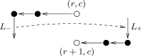
     (b) The path from $(r,c)$ to $(r+1,c)$

     

     (c) The new vertical and secondary links

     Figure 12: Stepping down from $(r,c)$ to $(r+1,c)$

     This series of movements is illustrated in Figure 12(b). Note that our sentinels at $(r,\pm\infty)$ ensure that the vertical links $L_{-}$ and $L_{+}$ will always exist.

  2. If required, insert the cell $(r+1,c)$ into the horizontal list for row $r+1$ and update its immediate horizontal neighbours.

  3. Insert the new vertical link $(r,c)\to(r+1,c)$, which we denote $L_{0}$.

  4. Replace the secondary link $L_{-}\to L_{+}$ with two secondary links $L_{-}\to L_{0}\to L_{+}$, as illustrated in Figure 12(c).

Operations (2), (3) and (4) are all constant time operations, but operation (1) may involve a lengthy walk through the data structure. The reason for the convoluted path (and indeed the secondary links) is because by walking backwards along each row we can ensure that operation (1) runs in amortised constant time, as shown in the following section.

4.3 Analysis of Running Time

Through the discussions of the previous section, we find that—with the single exception of the walk from $(r,c)$ to $(r+1,c)$ when we step down in the mapping matrix—each bit of the bitstream can be processed in constant time. The following lemma shows that these exceptional walks can be processed in amortised constant time, giving DistMatrix an overall running time of $O(n)$.

As in the previous section, we assume that we step down from $(r,c)$ to $(r+1,c)$; the arguments for the wraparound case $r=\beta-\alpha-1$ are essentially the same. It is also important to remember that the phrases step down and step right refer to the full movement when processing some bit of the bitstream, and not the many different links that we might follow through the data structure in performing such a step.

Lemma 4.7.

Consider the walk from cell $(r,c)$ to $(r+1,c)$ in the “step down” phase of the DistMatrix algorithm, as illustrated in Figure 12(b), and define the length of this walk to be the total number of links that we follow. After processing the entire bitstream, the sum of the lengths of all “step down” walks is $O(n)$. In other words, each such walk can be followed in amortised constant time.

Proof.

We prove this result using aggregate analysis, by “counting” the number of links in each walk using a rough upper bound. The following links are excluded from this count:

• all vertical and secondary links;

• the leftmost horizontal link on each row of each walk;

• any horizontal links that end at the starting point $(0,0)$;

• any horizontal links that end at the current cell $(r,c)$.

Figure 13 shows a sample walk where the excluded links are marked with dotted arrows, and the remaining links (all horizontal) are marked with bold solid arrows. It is clear that we exclude $O(n)$ links in total, and so if we can show that at most $O(n)$ horizontal links remain then the proof is complete.

Figure 13: Excluded links in a “step down” walk

Within each walk from $(r,c)$ to $(r+1,c)$, the horizontal links that remain have the following critical properties:

• The endpoint of each link in row $r$ is also the endpoint of some earlier step down. Moreover, this earlier step down was followed immediately by a succession of steps right that reached at least as far along the row as $(r,c)$.

• The endpoint of each link in row $r+1$ is also the beginning of some earlier step down. Moreover, this earlier step down was preceded immediately by a succession of steps right that originated at least as far back along the row as $(r+1,c)$.

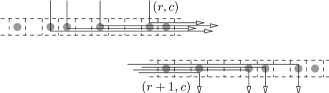
Figure 14: Earlier successions of steps associated with the remaining links

These properties are a consequence of our compression (recall that each non-sentinel cell that we store is either $(0,0)$, the current cell, a row entry or a row exit), as well as the fact that there are no vertical links between $L_{-}$ and $L_{+}$ that join row $r$ with row $r+1$. Figure 14 illustrates the successions of rightward steps that are described above.

We can now associate each remaining link $\ell$ with a position $\pi(\ell)$ in the bitstream:

• If the link $\ell$ is on the “upper” row $r$, consider the oldest sequence of steps that stepped down to the endpoint of $\ell$ and then right all the way across to $(r,c)$, as illustrated in Figure 15(a). We define $\pi(\ell)$ to be the position in the bitstream that was reached by this sequence when it passed through the cell $(r,c)$. Note that $0<\pi(\ell)\leq n$.

• If the link $\ell$ is on the “lower” row $r+1$, consider the oldest sequence of steps that stepped right from $(r+1,c)$ all the way across to the endpoint of $\ell$ and then down, as illustrated in Figure 15(b). We define $\pi(\ell)$ to be the position in the bitstream that was reached by this sequence when it passed through the cell $(r+1,c)$, negated so that $-n\leq\pi(\ell)<0$.

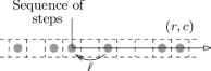
(a) If $\ell$ is on the upper row

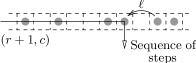
(b) If $\ell$ is on the lower row

Figure 15: The earlier sequence of steps that defines $\pi(\ell)$

The key to achieving an $O(n)$ total of walk lengths is to observe that the function $\pi$ is one-to-one:

• A link $\ell_{1}$ on the upper row of some walk can never have the same value of $\pi$ as a link $\ell_{2}$ on the lower row of some (possibly different) walk, since $\pi(\ell_{2})<0<\pi(\ell_{1})$.

• Within a single walk:

  • The values $\pi(\ell)$ for links $\ell$ on the upper row $r$ are distinct, because each corresponds to a different historical path through $(r,c)$, with a different initial entry point into row $r$.

  • Likewise, the values $\pi(\ell)$ for links $\ell$ on the lower row $r+1$ are distinct, because each corresponds to a different historical path along row $r+1$ with a different final exit point from row $r+1$.

• Between different walks:

  • Because we insert a new vertical link after every walk, each walk must have a distinct starting point $(r,c)$. The values $\pi(\ell)$ from the upper rows of different walks are therefore distinct because they correspond to positions in the bitstream for distinct cells $(r,c)$.

  • Likewise, the values $\pi(\ell)$ from the lower rows of different walks are distinct because they correspond to positions in the bitstream for distinct cells $(r+1,c)$.

Therefore $\pi$ is a one-to-one function. Because $\pi(\ell)\in\{-n,-n+1,\ldots,n-1,n\}$, it follows that the number of links $\ell$ in the domain of the function can be at most $2n+1$. Hence there are $O(n)$ horizontal links remaining that we have not excluded from our count, and the proof is complete. ∎

Through Lemma 4.7 we now find that each bit of the bitstream can be completely processed in amortised constant time, yielding the following final result:

Corollary 4.8.

The algorithm DistMatrix solves the fixed density problem in $O(n)$ time in the worst case.

5 Solving the Bounded Density Problem

We finish our suite of algorithms with a linear time solution to the bounded density problem, improving upon the log-linear DistSort algorithm of Section 3. Unlike our linear time solution to the fixed density problem, this algorithm is simple to express, uses no sophisticated data structures, and essentially involves just a handful of linear scans.

Once again we base our new algorithm on the distance sequence $d_{0},\ldots,d_{n}$. Recall from Lemma 3.4 that we seek the longest substring $x_{a},\ldots,x_{b}$ in the bitstream for which $d_{a-1}\leq d_{b}$. We begin with the following simple observation:

Lemma 5.1.

Suppose that $x_{a},\ldots,x_{b}$ is the longest substring of density $\geq\theta$ in our bitstream. Then there is no $i<a-1$ for which $d_{i}\leq d_{a-1}$, and there is no $i>b$ for which $d_{i}\geq d_{b}$.

The proof is simple—if there were such an $i$, then we could extend our substring to position $i$ and obtain a longer substring with density $\geq\theta$. This result motivates the following definition:

Definition 5.2 (Minimal and Maximal Position).

Let $k$ be a position in the bitstream, i.e., some integer in the range $0\leq k\leq n$. We call $k$ a minimal position if there is no $i<k$ for which $d_{i}\leq d_{k}$, and we call $k$ a maximal position if there is no $i>k$ for which $d_{i}\geq d_{k}$.

Figure 16 plots the distance sequence for the bitstream $1001101001011$ with target density $\theta=\alpha/\beta=3/5$, and marks the minimal and maximal positions on this plot.

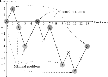
Figure 16: Minimal and maximal positions for the bitstream $1001101001011$

Minimal and maximal positions have the following important properties:

• They are the only positions that we need to consider. That is, the solution to the bounded density problem must be a substring $x_{a},\ldots,x_{b}$ for which $a-1$ is a minimal position and $b$ is a maximal position (Lemma 5.1).

• They are simple to compute in $O(n)$ time. To find all minimal positions, we simply walk through the distance sequence $d_{0},\ldots,d_{n}$ and collect positions $i$ for which $d_{i}$ is smaller than any distance seen before. To find all maximal positions, we walk through the distance sequence in reverse ($d_{n},\ldots,d_{0}$) and collect positions $i$ for which $d_{i}$ is larger than any distance seen before.

• They are ordered by distance. That is, if the minimal positions are $a_{1},a_{2},\ldots,a_{p}$ from left to right ($a_{1}<a_{2}<\ldots<a_{p}$) then we have $d_{a_{1}}>d_{a_{2}}>\ldots>d_{a_{p}}$. Likewise, if the maximal positions are $b_{1},b_{2},\ldots,b_{q}$ from left to right ($b_{1}<b_{2}<\ldots<b_{q}$) then we have $d_{b_{1}}>d_{b_{2}}>\ldots>d_{b_{q}}$. This is an immediate consequence of Definition 5.2.

Our algorithm then runs as follows:

1. We compute the distance sequence in $O(n)$ time, by incrementally adding $+(\beta-\alpha)$ or $-\alpha$ as seen in DistMap and DistSort.

2. We compute the minimal positions $a_{1},a_{2},\ldots,a_{p}$ and the maximal positions $b_{1},b_{2},\ldots,b_{q}$ in $O(n)$ time as described above.

3. For each minimal position $a_{i}$, we find the largest maximal position $b_{j}$ for which $d_{a_{i}}\leq d_{b_{j}}$. This gives a substring of density $\geq\theta$ and length $b_{j}-a_{i}+1$, and we compare this with the longest such substring found so far.

The key observation is that, because minimal and maximal positions are ordered by distance, step 3 can also be performed in $O(n)$ time. Specifically, if the minimal position $a_{i}$ is matched with the maximal position $b_{j}$, then the next minimal position $a_{i+1}$ will be matched with an equal or later maximal position, i.e., one of $b_{j},b_{j+1},\ldots,b_{q}$. We can therefore keep a pointer into the sequence of maximal positions and slowly move it forward as we process each of $a_{1},\ldots,a_{p}$, giving step 3 an $O(n)$ running time in total.

procedure PositionSweep($x_{1},\ldots,x_{n},\ \theta=\alpha/\beta$)     $d_{0}\leftarrow 0$ $\triangleright$ Compute the distance sequence     for $i\leftarrow 1$ to $n$ do          if $x_{i}=1$ then              $d_{i}\leftarrow d_{i-1}+(\beta-\alpha)$          else              $d_{i}\leftarrow d_{i-1}-\alpha$                   $p\leftarrow 1$ ; $a_{1}\leftarrow 0$ $\triangleright$ Compute minimal positions     for $i\leftarrow 1$ to $n$ do          if $d_{i}<d_{a_{p}}$ then              $p\leftarrow p+1$ ; $a_{p}\leftarrow i$                   $q\leftarrow 1$ ; $b_{1}\leftarrow n$ $\triangleright$ Compute maximal positions     for $i\leftarrow n-1$ downto $0$ do          if $d_{i}>d_{b_{q}}$ then              $q\leftarrow q+1$ ; $b_{q}\leftarrow i$                   $(a,b)\leftarrow(0,0)$ $\triangleright$ Best start/end found so far     $j\leftarrow 1$     for $i\leftarrow 1$ to $p$ do $\triangleright$ Run through minimal positions          while $j<q$ and $d_{a_{i}}\leq d_{b_{j+1}}$ do $\triangleright$ Find best maximal position              $j\leftarrow j+1$                    if $b_{j}-a_{i}>b-a+1$ then              $(a,b)\leftarrow(a_{i}+1,b_{j})$ $\triangleright$ Longest substring found so far                   Output $(a,b)$

Figure 17: The PositionSweep algorithm for the bounded density problem

We name this algorithm PositionSweep; see Figure 17 for the pseudocode. Through the discussion above we obtain the following final result:

Lemma 5.3.

The algorithm PositionSweep solves the bounded density problem in $O(n)$ time in the worst case.

6 Measuring Performance

We finish this paper with a practical field test of the different algorithms for the fixed density problem. In particular, because the linear DistMatrix algorithm involves a complex data structure with potentially significant overhead, it is useful to compare its practical performance against the log-linear but much simpler algorithms DistMap and DistSort. The tests are designed as follows:

• We use bitstreams of length $n=10^{8}$ for all tests. This value of $n$ was chosen to be large but manageable. We keep $n$ fixed merely to simplify the data presentation—additional data has been collected for several smaller values of $n$, and the results show similar characteristics to those described here.

• All bitstreams are pseudo-random. This is of particular benefit to the SkipMisMatch algorithm, whose expected running time of $O(n\log n)$ in a random scenario is significantly better than its worst case time of $O(n^{2})$.

• We run tests with several different values of the target density $\theta$. This includes values close to and far away from $\frac{1}{2}$, as well as values with small and large denominators—our aim is to identify to what degree the performance of different algorithms depends upon $\theta$. The values of $\theta$ that we use are $\frac{1}{2}$, $\frac{1}{3}$, $\frac{2}{5}$, $\frac{1}{5}$, $\frac{50}{101}$, $\frac{31}{101}$ and $\frac{1}{101}$.

• Each test involves the same 200 pre-generated bitstreams of length $n=10^{8}$. For each algorithm and each value of $\theta$ we measure the mean running time over all 200 bitstreams. All running times are measured as $\mathrm{user}+\mathrm{system}$ time, running on a single 3 GHz Intel Core 2 CPU with 4GB of RAM. All algorithms are coded in C++ under GNU/Linux.

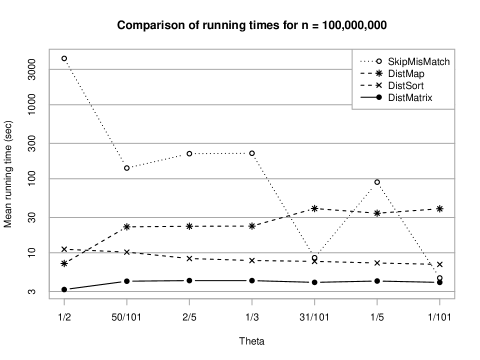
Figure 18: Running times of different algorithms for the fixed density problem

The results are plotted in Figure 18; note that the time axis uses a log scale, with each horizontal line representing a factor of approximately $\times 3$. Error bars are not included because most standard errors are within $\pm 1\%$; the only exceptions are for $\theta=\frac{1}{2}$, where DistMap has a standard error of $\pm 1.6\%$ and SkipMisMatch has a standard error of $\pm 10\%$. The values of $\theta$ are ordered by distance from $\frac{1}{2}$.

Happily, the results are what we hope for. The log-linear algorithms DistMap and DistSort perform significantly better than SkipMisMatch in most cases, and the linear algorithm DistMatrix consistently outperforms all of the others.

The dependency of SkipMisMatch upon $\theta$ is evident—performance is best when both $|\theta-\frac{1}{2}|$ and the denominator $\beta$ are large (as expected from Lemma 2.3), bringing it close to the 4 second running time of DistMatrix for the extreme case $\theta=\frac{1}{101}$. At the other extreme, for $\theta=\frac{1}{2}$ the SkipMisMatch algorithm runs orders of magnitude slower, with a mean running time of over an hour and some individual cases taking up to $10\frac{1}{2}$ hours.

Amongst the log-linear algorithms, we find that DistSort performs noticeably better than DistMap. Part of the reason is the memory overhead due to the map structure—it was found that DistMap often exceeded the available memory on the machine, burdening it with a reliance on virtual memory (which of course is much slower). The linear DistMatrix algorithm also suffers from memory problems to a lesser extent, but Figure 18 shows that that the effectiveness of the algorithm more than compensates for this. Figure 19 plots the peak memory usage for each algorithm, again averaged over all 200 bitstreams.

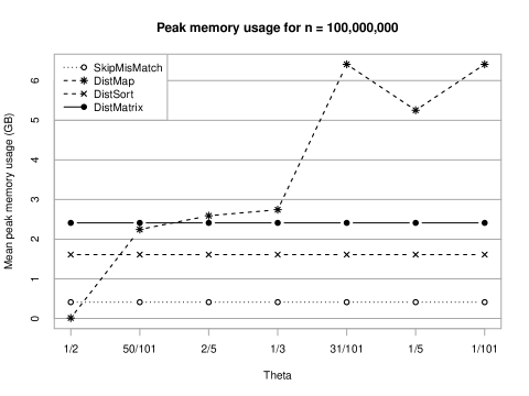
Figure 19: Peak memory usage of different algorithms for the fixed density problem

An interesting feature of the running times is that DistMap depends upon $\theta$ in an opposite manner to SkipMisMatch. This is because when $\theta\simeq\frac{1}{2}$ or the denominator $\beta$ is small, there are fewer distinct distances amongst $d_{0},\ldots,d_{n}$, and hence fewer elements stored in the map.

In conclusion, it is pleasing to note how consistently DistMatrix performs across all of the tested values of $\theta$, with mean running times ranging from $3.2$ seconds to $4.2$ seconds and standard errors of just $0.1\%$. The experiments therefore suggest that the added complexity and overhead of DistMatrix are well justified by the efficiency of the algorithm and its underlying data structure.

Benjamin A. Burton
School of Mathematics and Physics, The University of Queensland
Brisbane QLD 4072, Australia
(bab@debian.org)

References

- [1] R. Arratia, L. Gordon, and M. S. Waterman, The Erdős-Rényi law in distribution, for coin tossing and sequence matching, Ann. Statist. 18 (1990), no. 2, 539–570.
- [2] Giorgio Bernardi, Isochores and the evolutionary genomics of vertebrates, Gene 241 (2000), no. 1, 3–17.
- [3] Serdar Boztaş, Simon J. Puglisi, and Andrew Turpin, Testing stream ciphers by finding the longest substring of a given density, Information Security and Privacy, Lecture Notes in Comput. Sci., vol. 5594, Springer, Berlin, 2009, pp. 122–133.
- [4] Kevin Chen, Matt Henricksen, William Millan, Joanne Fuller, Leonie Simpson, Ed Dawson, HoonJae Lee, and SangJae Moon, Dragon: A fast word based stream cipher, Information Security and Cryptology—ICISC 2004, Lecture Notes in Comput. Sci., vol. 3506, Springer, Berlin, 2005, pp. 33–50.
- [5] Thomas H. Cormen, Charles E. Leiserson, Ronald L. Rivest, and Clifford Stein, Introduction to algorithms, 2nd ed., MIT Press, Cambridge, MA, 2001.
- [6] Laurent Duret, Dominique Mouchiroud, and Christian Gautier, Statistical analysis of vertebrate sequences reveals that long genes are scarce in GC-rich isochores, J. Mol. Evol. 40 (1995), no. 3, 308–317.
- [7] Paul Erdős and Alfréd Rényi, On a new law of large numbers, J. Analyse Math. 23 (1970), 103–111.
- [8] Stephanie M. Fullerton, Antonio Bernardo Carvalho, and Andrew G. Clark, Local rates of recombination are positively correlated with GC content in the human genome, Mol. Biol. Evol. 18 (2001), no. 6, 1139–1142.
- [9] Michael H. Goldwasser, Ming-Yang Kao, and Hsueh-I Lu, Linear-time algorithms for computing maximum-density sequence segments with bioinformatics applications, J. Comput. System Sci. 70 (2005), no. 2, 128–144.
- [10] Ronald I. Greenberg, Fast and space-efficient location of heavy or dense segments in run-length encoded sequences, Computing and Combinatorics, Lecture Notes in Comput. Sci., vol. 2697, Springer, Berlin, 2003, pp. 528–536.
- [11] Ross Hardison, Dan Krane, David Vandenbergh, Jan-Fang Cheng, James Mansberger, John Taddie, Scott Schwartz, Xiaoqiu Huang, and Webb Miller, Sequence and comparative analysis of the rabbit -like globin gene cluster reveals a rapid mode of evolution in a -rich region of mammalian genomes, J. Mol. Biol. 222 (1991), no. 2, 233–249.
- [12] Yong-Hsiang Hsieh, Chih-Chiang Yu, and Biing-Feng Wang, Optimal algorithms for the interval location problem with range constraints on length and average, IEEE/ACM Trans. Comput. Biol. Bioinformatics 5 (2008), no. 2, 281–290.
- [13] Donald E. Knuth, The art of computer programming, Vol. 2: Seminumerical algorithms, 3rd ed., Addison-Wesley, Reading, MA, 1997.
- [14] Yaw-Ling Lin, Tao Jiang, and Kun-Mao Chao, Efficient algorithms for locating the length-constrained heaviest segments, with applications to biomolecular sequence analysis, Mathematical Foundations of Computer Science 2002, Lecture Notes in Comput. Sci., vol. 2420, Springer, Berlin, 2002, pp. 459–470.
- [15] G. Marsaglia, A current view of random number generators, Computer Science and Statistics: The Interface (L. Billard, ed.), Elsevier Science, Amsterdam, 1985, pp. 3–10.
- [16] David R. Musser, Introspective sorting and selection algorithms, Softw. Pract. Exper. 27 (1997), no. 8, 983–993.
- [17] Paul M. Sharp, Michalis Averof, Andrew T. Lloyd, Giorgio Matassi, and John F. Peden, DNA sequence evolution: The sounds of silence, Phil. Trans. R. Soc. Lond. B 349 (1995), no. 1329, 241–247.
- [18] Serguei Zoubak, Oliver Clay, and Giorgio Bernardi, The gene distribution of the human genome, Gene 174 (1996), no. 1, 95–102.