Efficient Random Walk Algorithm for Simulating Thermal Transport in Composites With High Conductivity Contrast

Abstract

In dealing with thermal transport in composite systems, high contrast materials pose a special problem for numerical simulation: the time scale or step size in the high conductivity material must be much smaller than in the low conductivity material. In the limit that the higher conductivity inclusion can be treated as having an infinite conductivity, we show how a standard random walk algorithm can be alterred to improve speed while still preserving the second law of thermodynamics. We demonstrate the principle in a 1D system, and then apply it to 3D composites with spherical inclusions.

I Introduction

A variety of systems display dramatically different thermal diffusivities. For example, the thermal conductivity is estimated at 3000 W/mK for an isolated multiwall carbon nanotube (CNT) and between 1750 and 6600 W/mK for a single wall carbon nanotube at room temperature.ESChoi ; JChe ; JHone ; SBerber Typical polymer matrices, in contrast, have thermal conductivities that are three orders of magnitude smaller. Composites using carbon nanotubes have been suggested as cheap materials with average thermal conductivity.RBBird However making improved thermal conducting polymer composites has been hindered due to the Kapitza thermal resistance and various processing issues.

It may be possible to alter this resistance through functionalizing the ends or surface of the CNTs, although this may decrease the thermal conductivity of the material. The problem of optimizing the thermal conductivity of CNT composites presents an intriguing combination of high conductivity contrast, strong disorder, and incorporated materials with an extremely high aspect ratio. Thus an efficient and reliable method to calculate effective thermal conductivity and varying interface resistance in this two phase medium is desirable.

This problem has been studied in the context of electrical conductivity.elect1 ; elect2 However, the inclusions in thermal transport can have be quite asymmetric and entangled. In these cases it the isotropic averaging models may not apply.

One approach to model the thermal transport in composites is to use a random walk algorithm in which the transport is assumed to be diffusive. For instance, Tomadakis and Sotirchos Toma1 ; Toma2 has used this approach to find the effective transport properties of random arrays of cylinders in a conductive matrix. Recently, Doung et.al cnt1 ; cnt2 ; cnt3 developed a random walk algorithm to model thermal transport in carbon nanotube-polymer composites and the simulation results showed a reasonable agreement with the experimental data for Epoxy-SWNT compositescnt2 . In this approach thermal transport is described by random jumps of thermal markers carrying a certain amount of energy ($\Delta E$). The step size($\Delta x=x_{2}-x_{1}$) of this thermal markers follows the gaussian distribution.(See Eq.1) The standard deviation ($\sigma$) of the gaussian step distribution in each one of the space dimensions is $\sigma_{M/I}=\sqrt{2D_{M/I}\Delta t}$, where $\Delta t$ is the time increment, $M/I$ refers to matrix or inclusions and $D_{M/I}$ is the thermal diffusivity. However problem arises when their is a high contrast in thermal diffusivity of matrix and inclusions. The step size in highly conducting inclusions $\Delta x_{I}$ become very large compare to the that of poorly conducting matrix $\Delta x_{M}$. Eventually this leads the markers to jump out the inclusions as soon as they enter. This can be avoided having very small steps inside the matrix so that the steps inside the inclusions are within the dimensions of the inclusions. But this is computationally expensive.

When the thermal diffusivity of the inclusion is very high relative to the matrix it is reasonable to assume that the thermal diffusivity of the inclusions is infinite. This obviates the need to model random walks inside the inclusions. In this approach markers entering an infinite conductivity inclusion (ICI) are distributed uniformly inside the inclusion on the next time step. Some fraction will leave on the next time step and they always leave from the surface of the inclusion. (Otherwise the simulation wastes time on walkers that hop within the ICI.) However, we must be careful in choosing how the walkers leave the the ICI since incorrect approaches can lead to the unphysical result of a system at uniform temperature spontaneously developing a temperature gradient at the interface between the inclusion and the medium.cnt2 While the effect is apparently small, it must be remembered that diffusion occurs at these same interfaces. In this paper we provide a rigorous approach for implementing a random walk algorithm with emphasis on the treatment at the interface between the inclusions and the matrix material for high conductivity contrast composites, and we quantify the errors made when gaussian and modified step distributions are employed.

This paper is divided into four parts. In the first, we briefly describe the algorithm for “infinite conductivity” inclusions. Next, we show the rigorous way to handle inclusions in one dimensional systems. We verify our results numerically in ordered and disordered systems, and compare them to results obtained by assuming that the walkers leave the surface with a gaussian step distribution. In the next section we develop this approach to spheres in three dimensions and again verify it numerically, showing quantitatively the errors that develop if a gaussian step distribution from the surface is used. Interestingly, the errors in thermal conductivity are larger in 3D than in 1D and larger for random arrays than for regular ones. In the final section we conclude with a summary and a discussion of future work.

II The Model

The goal is to calculate the thermal conductivity of a composite composed of a matrix containing a distribution of “infinite conductors” (ICs). This conductivity is calculated by fixing the heat flux through the computational volume and measuring the resulting average temperature gradient. The diffusion of heat is modelled by the motion of random walkers within the domain. The computational cell is divided in bins, and the temperature distribution is calculated from the number of walkers in each bin. To maintain a constant heat flux in the $x$ direction through the computational cell, random walkers carrying $+\Delta E$ energy are periodically added at the surface $x=x_{\mathrm{min}}$, and then allowed to move with random jumps that follow a gaussian distribution into the computational cell. In order to fix an “outward” energy flux on the opposite surface, random walkers carrying $-\Delta E$ energy are added at the surface $x=x_{\mathrm{max}}$ at the same rate as the positive markers. The $+\Delta E$ and $-\Delta E$ thermal markers are often called ”hot” and ”cold” walkers. The exact size of $\Delta E$ is arbitrary: the heat flux might be modelled by many small walkers or one large one. However using too many walkers is computionally ineffcient, while too few produces noisy results that requires more runs to get better averages. In the $y$ and $z$ direction the computaional domain is assumed to be periodic. The solution at steady states yields a linear temperature profiile and the thermal conductivity can be extracted from Fourier’s law. To incorporate the effect of the Kapitza thermal resistance, walkers in the matrix that would normally attempt to jump into the IC can only do so with a probability $f_{m,IC}$.Kap ; Shen ; JLB ; CJTwu Thus they stay in the matrix phase with a probability $1-f_{m,IC}$. The value of $f_{m,IC}$ is determined by the Kapitza resistance. This can be estimated using acoustic mismatch model when the physical properties of the materials are known.SchwartzPohl

Similarly, random walkers located within the IC have a probability to hop out on each time step. Exactly what fraction of the walkers should leave in each time step, and the exact nature of the probability distribution for the steps they should take from the surafce are determined in the next two sections. However, those that do leave, exit at random positions on the IC. This is done to model the “infinite” conductivity of IC so that the walker distribution within the IC is uniform.

Collisions between walkers are ignored. The random walk reflects the scattering of phonons in the disordered matrix material. Walker-walker scattering would reflect nonlinear thermal conductivities which are typically small. Similarly, we assume that the properties of the materials (e.g. density, specific heat, thermal relaxation length) do not change with temperature over the range modelled.

Finally, we assume that the product of the mass density of IC and specific heat capacity equals that of the matrix, so that in thermal equilibrium the walker density would be uniform inside and out of the IC’s. This is done for simplicity, so that the local temperature is simply proportional to the difference of the average density of hot and cold walkers. Without this assumption we would have to alter the probability of walkers entering and leaving the IC’s so that in thermal equilibrium, the ratio of average walker density inside the IC to that of the matrix equals the ratio of their volumetric heat capacities. Only then would the equilibrium walker distribution represent a uniform temperature.

III Random walks with infinite conductivity inclusions in 1D.

Below we describe how to efficiently handle the random walks in a fashion that satisfies the second law of thermodynamics. The difficulty lies in properly handling the random walkers that jump out from the high conductivity material. To make the explanation clear, we first look at the one dimensional case. We subsequently address the three dimensional case for spherical inclusions in section IV.

III.1 Analytic results for one dimensional walks

We consider a set of random walkers moving in a one dimensional ring, half made from an “infinitely conducting material” as show in fig.1. We can view this as a one dimensional line with boundaries at $x=\pm 1$. We know that in equilibrium the density of random walkers throughout the whole ring should be uniform.

Consider a surface located at $x=s$, as shown in fig.1.b. The flux of random walkers from the left through the surface must equal that from the right. This is not a problem for a surface located near the center of the interval. However, if $1>\sigma>1-s$, the flux of random walkers from right in the matrix medium cannot balance those from the left; there are too few of them. The solution lies in that the difference must be made up from random walkers leaving the “infinite” conductivity material. If they were distributed uniformly throughout the infinite conducting material, their flux would maintain the equilibrium.

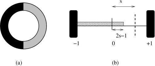
Figure 1: An illustration of the one dimensional model. In (a) the darker material on the left is of “infinite” conductivity. The one dimesional system therefore has two boundaries as shown in (b), where we assume $\sigma<<1$. The difficulty is that in equilibrium the net flux through any surface (e.g. the dashed line) must be zero. Walkers hopping through the surface from the shaded region in Fig.(b) must be balanced by walkers leaving the right hand infinite conductor. This implies that if random walkers always leave the surface of the infinite conductor (IC), they must have a different jump distribution than random walkers inside the “normal” region.

We do not wish to model the inside of the IC inclusions because random walkers within them move on a much faster time scale than those outside. We assume that a random walker instantly leaves from any point on the surface (in this case from $x=\pm 1$). However, since they leave always exactly from the surface, their step distribution must be different from that of random walkers within the matrix medium.

In each step of the simulation we move the walkers inside the interval $-1<x<1$, as well as those outside. We wish to do this in a fashion that is in agreement with the second law of thermodynamics. Let the probability that a walker in the matrix medium jumps from $x_{1}$ to $x_{2}$ be given by:

$$P(x_{1},x_{2})={\frac{1}{\sqrt{2\pi}\sigma}}e^{\frac{-(x_{2}-x_{1})^{2}}{2\sigma^{2}}}$$ (1)

In each time interval we can see that only a fraction of the walkers inside the IC will leave, or else their density would not equal that in the normal medium. In this simple model, we require that the number inside the matrix medium ($N_{i}$) equals that outside ($N_{o}$) in the IC. We also require that the net flux through a surface located at $x=s$ is zero.

The flux to the left from particles lying in the matrix region, $s<x<1$ is balanced by the flux to the right for those lying between $2s-1<x<s$. However those in the shaded region of fig.1 are not so compensated. They must be balanced by a net flux of walkers leaving the righthand boundary. Denote the flux from the shaded region to the right by $N_{r}$; it is :

$$N_{r} = \rho_{0}\int_{-1}^{2s-1}dx_{1}\int_{s}^{\infty}dx_{2}P(x_{1},x_{2})$$ (2)

$$= {\frac{\rho_{0}}{2}}\int_{0}^{\infty}\mathrm{\,Erfc\,{\left(\frac{z-s+1}{\sqrt{2}\sigma}\right)}}\,dz$$ (3)

where $\mathrm{\,Erfc\,{(x)}}$ is the complementary error function, $\mathrm{\,Erfc\,{(x)}}=1-\mathrm{\,Erf\,{(x)}}$. We are summing over any walker starting in the shaded region ending up anywhere to the right of the barrier. We have let the upper limit of the endpoint of the jump to infinity since $\sigma<<1$; we extend the lower limit of the first integral to $-\infty$, and we have shifted variables to $z=2s-1-x_{2}$. We neglect any walkers leaping from the IC on the left boundary $x=-1$ all the way through $s$.

The flux $N_{r}$ must be balanced by the flux from walkers leaving the IC on the right. Let the probability that a random walker in the IC leaves it be given by $\lambda$, and the probability that it jumps to a point $x$, leaving from the right hand boundary, be $f(x)$. Then the flux to the left through the surface at $x=s$ due to these walkers is

$$N_{\ell}=N_{o}\lambda\int_{-\infty}^{s}f(x)\,dx$$ (4)

We set $N_{\ell}=N_{r}$, and take the derivative of both sides with respect to $s$. This gives us an integral expression for $f(s)$:

$$f(s)={\frac{\rho_{0}}{2N_{0}\lambda}}\left[\mathrm{\,Erf\,{\left(\frac{s-1}{\sqrt{2}\sigma}\right)}}+1\right]$$ (5)

The requirements that $N_{i}=N_{o}$ and the balancing of the fluxes when $s=1$ is enough to solve for $f(s)$. The distribution of steps, $\tilde{f}(u)\equiv f(1-u)$ is given by:

$$\tilde{f}(u)=\sqrt{\frac{\pi}{2}}{\frac{1}{\sigma}}\left(1-\mathrm{\,Erf\,{\left(\frac{u}{\sqrt{2}\sigma}\right)}}\right)$$ (6)

III.2 Numerical results for thermal conductivity in 1D

The above analytical calculation provides the correct step distribution for walkers leaving the edge of the infinite conductors. We can compare it to a simple model where we simply have the walkers take a step with a Gaussian probability distribution (mean size 0.20) from the surface. Fig.2 is the spatial distribution of random walkers in such a one dimensional system.probability Plotted are the average number of walkers in each of 20 bins, equally spaced $-1<x<1$ over the course of $10^{5}$ Monte Carlo steps. Starting with 500 random walkers, half should be in the “matrix” region, so that the average number/bin should be 12.5. The dashed line is the result of performing the simulation incorrectly, and letting the walkers have a Gaussian step distribution as in eq.1; There are too many walkers in the interval, and their distribution is not uniform. The solid line is the result of using eq.6, which yields the correct result, and is uniform.

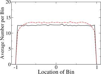
Figure 2: (Color online) Results for the one dimensional model of a random walk on a ring with an infinite conductivity inclusion. The steps in the random walk have a Gaussian distribution with a mean of $0.20$. Plotted are the average number of walkers in each of 20 bins, equally spaced $-1<x<1$ over the course of $10^{5}$ Monte Carlo steps. Starting with 500 random walkers, half should be in the “normal” region, so that the average number/bin should be 12.5. The dashed line is the result of performing the simulation incorrectly, and letting the walkers have a Gaussian step distribution as in eq.1; There are too many walkers in the interval, and their distribution is not uniform. The solid line is the result of using eq.6, which yields the correct result.

In order to determine the significance of this error, we place several ICs in the computational volume and run at constant heat flux until the temperature distribution converges. We then extract the gradient in walker density and calculate the thermal conductivity. Sample results are plotted in fig.(3), where we show the results for Gaussian steps (lower curve) and steps governed by eq.(6) (upper curve). The latter gives physically reasonable results (with noise), in which the temperature is constant the ICs and uniformly decreasing in the matrix.

The thermal conductivity is extracted from the ratio of the slope of the temperature (the walker density) to the applied flux. In fig.(4 ) we plot the average value of the percent error in the thermal conductivity as a function of the transmission probability, $f_{m,IC}$, for regular and random 1D arrays. In this simulation the ICs were 0.50 units long and the material between them was 1.00 units wide. The results are averaged over five runs each lasting for 40,000 time steps. The percent error is defined as the difference between the results of simulations using the Gaussian steps and the results using eq.6. The error bars represent the variation in thermal conductivities over the runs. Thus we see that the error can range as large as five percent, and that can vary substantially.

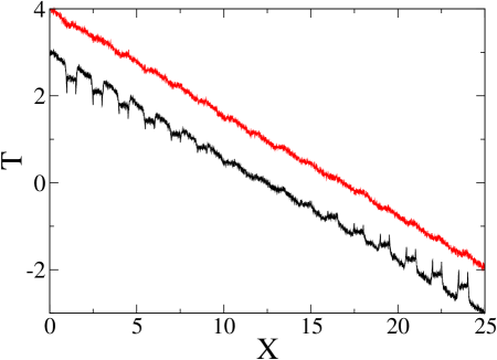
Figure 3: (Color online) Plots of the temperature distribution in a periodic array of infinite conductivity inclusions in a 1D matrix. The temperature is determined by the average of the difference between the number of positive and negative walkers in a given region. This plot was generated over a run of 62,500 time steps where 10,000 positive (negative) walkers were added every 10 time steps at the left (right) border. The ICs are 0.50 units long and the matrix spacer between them is 1.00 units. The probability to cross into an IC from the matrix is 0.16. Lower line: The temperature distribution generated by having random walkers depart the ICs with Gaussian steps. Upper line: The temperature distribution (shifted up one unit for clarity) given by an algorithm using the step probability distribution of eq.6. Note that temperature gradients spontaneously appear at interfaces when the incorrect jump distribution is used.

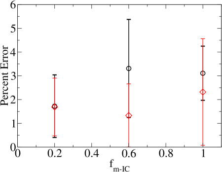
Figure 4: (Color online) Plot of the relative percent error for the the thermal conductivity calculated using a Gaussian step distribution ($\sigma=0.1$) as compared to that of eq.(6) as a function of $f_{m-IC}$, the probability for a walker to enter into an inclusion. The results are for a one dimensional system with 20 inclusions; the diamonds are for a regular array of ICs and the circles are random ICs. The error bars are based on a sample of five different configurations and are included to give an indication of how large the the errors can be.

IV Three dimensional models

We have shown above that errors in one dimensional simulations are avoidable, but only a few percent. Below we generalize the above problem to three dimensions for spherical inclusions, and show that the effect can be significant.

IV.1 Analytic Derivation of Random Walks with Spherical Inclusions

In our model random walkers that land inside the sphere are immediately moved to a random point on the surface of the sphere. On the next time step they can move in the radial direction away from the sphere. We assume that if we choose the fraction that leave and their step distribution correctly, then when we are in equilibrium we will obtain a uniform, stationary density outside and inside the sphere.

The number of random walkers entering the sphere from a region $d\vec{r}$ near $\vec{r}\,$ landing inside the sphere is given by:

$$n(\vec{r})=\,d\vec{r}\,\,\,{\frac{\rho_{0}f_{k}}{(2\pi)^{3/2}\sigma^{3}}}\int_{r^{\prime}<R}d\vec{r^{\prime}}\,e^{\frac{-(\vec{r}-\vec{r^{\prime}})^{2}}{2\sigma^{2}}}$$ (7)

where we have generalized the probability distribution of eq.(1) to three dimensions. The factor $f_{k}$ represents the Kapitsa resistance; it is the probability that a random walker will enter the spherical inclusion. When $f_{k}=0$, no walkers enter the inclusion and the Kapitsa resistance is infinite; when $f_{k}=1$ then walkers can freely step into the inclusion and the Kapitsa resistance is zero. The total number entering a sphere of radius $R$ is

$$N_{\mathrm{in}}(R)=\int_{r>R}d\vec{r}\,\,\,{\frac{\rho_{0}f_{k}}{(2\pi)^{3/2}\sigma^{3}}}\int_{r^{\prime}<R}d\vec{r^{\prime}}\,e^{\frac{-(\vec{r}-\vec{r^{\prime}})^{2}}{2\sigma^{2}}}$$ (8)

For any value of ${\vec{r}}$ we can rotate our primed coordinate system so that $\hat{z}^{\prime}\parallel{\vec{r}}$ so that the angle between ${\vec{r}}$ and ${\vec{r}\,^{\prime}}$ is simply $\theta^{\prime}$, the spherical polar angle in the primed system. The angular integrals can then all be done in closed form giving

$$N_{\mathrm{in}}(R)=\sqrt{8\pi}\,{\frac{\rho_{0}f_{k}}{\sigma}}\int_{r>R}r\,dr\int_{r^{\prime}<R}r^{\prime}dr^{\prime}\,\left(e^{\frac{-(r+r^{\prime})^{2}}{2\sigma^{2}}}-e^{\frac{-(r-r^{\prime})^{2}}{2\sigma^{2}}}\right)$$ (9)

The resulting integral can also be found exactly yielding

$$N_{\mathrm{in}}(R)={\frac{2}{3}}\rho_{0}f_{k}\left[\sqrt{2\pi}\sigma\left(3R^{2}-\sigma^{2}\right)+2\pi R^{3}\,\mathrm{\,Erfc\,{({\frac{\sqrt{2}R}{\sigma}})}}+\sqrt{2\pi}\sigma e^{\frac{-2R^{2}}{{\sigma^{2}}}}(\sigma^{2}-R^{2})\right]$$ (10)

If the density of walkers is uniform then the number inside the sphere is $V_{s}\rho_{0}$ where $V_{s}$ is the volume of the sphere. (This is only true when the product of the density and specific heat capacity of the matrix and IC’s are equal. When this constraint does not hold the number of walkers inside the IC is $V_{s}\rho_{0}\frac{C_{M}\rho_{M}}{C_{IC}\rho_{IC}}$. Where $C_{IC}$($C_{M}$) and $\rho_{IC}$($\rho_{M}$) are specific heat capacity and mass density of the IC(Matrix).) In each time step we allow a fraction $\lambda$ of them to leave. In equilibrium the flux into the sphere (Eq.10) equals the flux out ($V_{s}\rho_{0}\lambda$), allowing us to calculate $\lambda$:

$$\lambda={\frac{2}{3}}{\frac{f_{k}}{V_{s}}}\left[\sqrt{2\pi}\sigma(3R^{2}-\sigma^{2})+2\pi R^{3}\mathrm{\,erfc\,{({\frac{\sqrt{2}R}{\sigma}})}}+\sqrt{2\pi}\sigma e^{\frac{-2R^{2}}{{\sigma^{2}}}}(\sigma^{2}-R^{2})\right]$$ (11)

When $R>>\sigma$, we expect the geometry of the inclusion to be irrelevant. In this limit, if the random walkers had a flat distribution of steps bounded by $\sigma$, then the flux into the sphere would come from a thin spherical shell of thickness $\sigma$ and radius $R$. The volume of this shell is $\sigma A_{s}$, where $A_{s}$ is the surface area of the sphere. The flow in from this shell is balanced by the flow out of the volume, $V_{s}\rho\lambda$. It is useful to write this in terms of a new constant, $c_{0}$, defined via

$$c_{0}\equiv{\frac{\lambda V}{\sigma A}}$$ (12)

which is dimensionless and becomes shape independent as $\sigma\to 0$. In this case

$$c_{0}=f_{k}\left[{\frac{1}{\sqrt{2\pi}}}\left(1-{\frac{\sigma^{2}}{3R^{2}}}\right)+{\frac{R}{3\sigma}}\mathrm{\,erfc\,{({\frac{\sqrt{2}R}{\sigma}})}}\right]$$ (13)

This quantity is bounded by $f_{k}/\sqrt{2\pi}$, the result one would get for an infinite slab. The factor $1/\sqrt{2\pi}$ arises from the fact that walkers have a gaussian distribution of step sizes, and not a flat one.

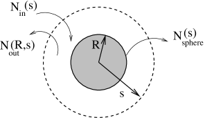
Figure 5: An illustration of the three dimensional model for spheres. The grey material is a sphere of “infinite” conductivity with radius $R$. We wish to calculate the distribution of steps sizes taken by random walkers leaving the surface of the sphere. We do this by requiring that in equilibrium the net flux through any surface (e.g. the dashed line indicating a sphere of radius $s$) must be zero. The number of walkers hopping in through the dotted surface ($N_{in}(s)$) must be balanced by the total number of walkers hopping out, both those from the matrix material ($N_{out}(R,s)$) and those from the surface of the sphere ($N_{\mathrm{sphere}}(s)$). This condition allows us to calculate the step distribution.

Next we have to calculate the distribution of steps for random walkers leaving the surface of the sphere. As in the one dimensional case of subsection III.1 above, we can calculate the desired result by balancing fluxes in equilibrium. We draw an imaginary surface of radius $s$ about the spherical inclusion. In equilibrium, the net flux through this surface must be zero, as illustrated in fig.(5).

$$N_{in}(s)=N_{out}(R,s)+N_{\mathrm{sphere}}(R,s)$$ (14)

The flux in through the sphere of radius $s$, $N_{in}(s)$, is the result eq.( 10) evaluated for a radius of $s$. The flux outward from the matrix material is given by the integral:

$$N_{\mathrm{out}}(R,s)=\int_{R<r<s}d{\vec{r}}{\frac{\rho_{0}f_{k}}{(2\pi)^{3/2}\sigma^{3}}}\int_{r^{\prime}>s}d\vec{r}\,^{\prime\frac{-(\vec{r}-\vec{r}\,^{\prime 2})}{2\sigma^{2}}}$$ (15)

We can again evaluate this integral analytically to obtain:

$$N_{\mathrm{out}}(R,s)={\frac{2}{3}}f_{k}\rho_{0}\left[2\pi s^{3}\mathrm{\,erfc\,{(\frac{\sqrt{2}s}{\sigma})}}+\sqrt{2\pi}\sigma(\sigma^{2}-s^{2})e^{\frac{-2s^{2}}{\sigma^{2}}}-\sqrt{2\pi}\sigma(\sigma^{2}-3s^{2})\right.$$

$$\left.+\sqrt{2\pi}\sigma(\sigma^{2}-s^{2}-R^{2}-Rs)e^{\frac{-(s-R)^{2}}{2\sigma^{2}}}-\sqrt{2\pi}\sigma(\sigma^{2}-s^{2}-R^{2}+Rs)e^{\frac{-(s+R)^{2}}{2\sigma^{2}}}\right.$$

$$\left.+\pi(s^{3}-R^{3})\mathrm{\,erfc\,{(\frac{s-R}{\sqrt{2}\sigma})}}-\pi(s^{3}+R^{3})\mathrm{\,erfc\,{(\frac{s+R}{\sqrt{2}\sigma})}}\right]$$ (16)

Finally, we can write an expression for the flux of random walkers (originating on the inclusion surface) that hop out through the sphere of radius $s$:

$$N_{\mathrm{sphere}}(s)=V_{s}\rho_{0}\lambda\int_{s}^{\infty}f(r)\,dr$$ (17)

where $f(r)\,dr$ gives the fraction of walkers that jump radially outward to a distance between $r$ and $r+dr$ from the center of the inclusion.

Eqns.(10), (16) and (17) give us enough information to calculate the step distribution function $f(r)$. However in computer applications we do not actually use $f(r)$. Rather algorithms typically generates a random number, $p$, in a flat distribution $0<p<1$, and use that to select a random step $\delta(p)$ from the center of the sphere, $\delta>R$. We can do this by first calculating the integral of $f(r)$:

$$P(\delta)\equiv\int_{R}^{\delta}f(r^{\prime})\,dr^{\prime}$$ (18)

Note that $P(R)=0$ and $\lim_{\delta\to\infty}P(\delta)=1$. We then must invert this functional relationship to get $\delta(P)$, which gives us the step generating function we desire. We note that from eq.(17) and (18) we have:

$$N_{\mathrm{sphere}}(R,s)=V_{s}\,\rho_{0}\lambda\left[1-P(s)\right]$$ (19)

Equating this via eq.(14) and dropping exponentially small terms we have

$$P(s) = 1-$$ (20)

$${}\left[\pi(R^{3}-s^{3})\mathrm{\,erfc\,}{\left({\frac{{s-R}}{{\sqrt{2}\sigma}}}\right)}-\sqrt{2\pi}\sigma(\sigma^{2}-s^{2}-R^{2}-Rs)e^{\frac{{-(s-R)^{2}}}{{2\sigma^{2}}}}\right.$$

$$\frac{{}+\left.\sqrt{2\pi}\sigma(\sigma^{2}-s^{2}-R^{2}+Rs)e^{\frac{-(s+R)^{2}}{2\sigma^{2}}}+\pi(s^{3}+R^{3})\mathrm{\,erfc\,}{\left(\frac{s+R}{\sqrt{2}\sigma}\right)}\right]}{{\displaystyle{\sqrt{2\pi}\sigma(3R^{2}-\sigma^{2})+\sqrt{2\pi}\sigma(\sigma^{2}-R^{2})e^{\frac{-2R^{2}}{\sigma^{2}}}+2\pi R^{3}\mathrm{\,erfc\,}\left(\frac{\sqrt{2}R}{\sigma}\right)}}}$$

This result has the desired behavior at the limits, $P(R)=0$ and $\lim_{s\to\infty}P(s)=1$. This function is not analytically invertible; in implementation it is evaluated on a mesh and the inverse is calculated via interpolation.

IV.2 Numerical Results in 3D

We implemented a random walk algorithm in three dimensions similar to that of section III above. In three dimensions we applied periodic boundary conditions in the $y$ and $z$ directions. A temperature profile in the $x$ direction was obtained simply by binning all walkers in a given range of $x$ for all $y$ and $z$; such slices would cross inclusions as well as matrix material. Walkers that were labelled as inside a given inclusion were assigned a random position inside the inclusion for the purpose of doing this averaging. The simulation volume was $10\times 10\times 10$, and the random walk in the matrix was described by a Gaussian distribution with a rms value of 0.10 in these units. The transition probability $f_{m,IC}$ was fixed at 1.0.

In fig.(6) the percent error (defined as the ratio of the difference of thermal conductivities measured using the Gaussian step distribution and that of eq.(20), divided by the former) is plotted as a function of the volume fraction of infinite conductivity inclusions, for a fixed surface area for the inclusions. (If there were only a single spherical inclusion, it would have had a volume fraction of 5%.)fudge As the number of inclusions at fixed surface area increases, their total volume decreases as $N^{-3/2}$. (For example, the largest volume fraction, 0.20, corresponds to $100$ spheres of radius $0.9772$). The results at several values of $N$ were calculated for five random configurations and the average and standard deviation are plotted. The effect of using a simplified step distribution is larger in three dimensions, and can affect the results by up to 18%.

The percent error was also calculated as a function of the surface area for fixed volume fraction and plotted in fig.(7). The volume fraction was fixed at 5%, and the surface area increases with $N$ as $N^{2/3}$. Five simulations were run for $N=100,200,\dots 1000$ and the average and standard deviation were plotted as a function of the surface area relative the minimum surface area, $A_{0}$, the area of a sphere that is 5% of the volume. Again, the effect of using the wrong simulation algorithm is shown to be substantial.

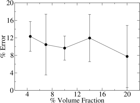
Figure 6: Plot of the percent error in the thermal conductivity as a function of the volume fraction for fixed surface area. The percent error is defined as the ratio of the difference of thermal conductivities measured using the Gaussian step distribution and that of eq. (20) divided by the former. Note that the error varies only slightly with volume fraction.

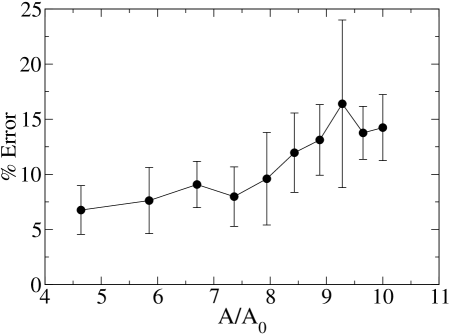
Figure 7: Plot of the percent error in the thermal conductivity as a function of the surface area of the spherical inclusions at a fixed volume fraction of 5%. The surface area is measured in terms of $A_{0}$, the surface area of a sphere with 5% of the total volume. The percent error is defined as the ratio of the difference of thermal conductivities measured using the Gaussian step distribution and that of eq.(20). divided by the former.

V Conclusions and Future work

Transport in composites with a large disparity in conductivities is important to a large number of systems. In this paper we have demonstrated an efficient and physically sound algorithm for calculating effective conductivities of composites with large contrasts in conductivity. We have shown that the errors introduced are small but measurable in one dimension, and moderately significant in 3D.

The spherical inclusion case is the simplest 3D problem, but not the most relevant to many systems. Carbon nanotubes might be approximated as cylinders, to lowest order. However, in that case the 1D integrals of section(IV.1) become more complicated and handling the endcaps of the cylinders becomes problematic. A simple approach might be to simply ignore transport through the endcaps, or treat a nanotube as an extremely prolate spheroid so that diffusion from the inclusion can again be treated as a one dimensional walk normal to the surface. These approximations are the subject of current research.

- (1) E.S.Choi, J.S.Brooks, and D.L.Eaton, J.Appl.Phys. 94 6034(2003).
- (2) J.Che,T.Cagin, and W.A.Goddard III,Nanotechnology(2003).
- (3) J.Hone,B.Batlogg, Z.Benes, A.T.Jonson, and J.E.Fischer, Science 289, 1730(2000).
- (4) S.Berber, Y.K.Kwon, and D.Tomanek, Phys. Rev. Lett. 84,4613(2000).
- (5) R. B. Bird, W. S. Stewart, and E. N. Lightfoot, Transport Phenomena, 2nd ed. (Wiley, New York, 2002),pp.282,376 and 397.
- (6) E. H. Kerner, 1956 Proc. Phys. Soc. B 69 802
- (7) Lawrence E. Nielsen, Ind. Eng. Chem. Fundamen., 1974, 13 (1), 17.
- (8) M. M. Tomadakis and S. V. Sotirchos, J. Chem. Phys. 98, 616 (1992).
- (9) M. M. Tomadakis and S. V. Sotirchos, J. Chem. Phys. 104, 6893 (1996).
- (10) M. H. Duong, D. V. Papavassiliou, K. J. Mullen and L. L. Lee, Appl. Phys. Lett. 87, 013101(2005).
- (11) M. H. Duong, D. V. Papavassiliou, K. J. Mullen and S. Maruyama, Nanotechnology 19, 065702 (2008).
- (12) H. M. Duong, D. V. Papavassiliou, K. J. Mullen, B. L. Wardle, S. Maruyama, Inter. J. of Heat and Mass Transfer, 52 (2009) 5591-5597.
- (13) P. L. Kapitza, J. Phys. (USSR) 4,181 (1941).
- (14) S. Shenogin, L. Xue, R. Ozisk, P. Keblinski, and D. G. Cahill, J. Appl. Phys. 95, 8136(2003).
- (15) J. L. Barrat and F. Chiaruttini, Mol.Phys. 101 ,1605(2003).
- (16) C. J. Twu and J. R. Ho, Phys. Rev. B 67, 205422 (2003).
- (17) E. T. Swartz, and R. O. Pohl, Rev. Mod. Phys. 1989, 61 (3), 605.
- (18) The function gives the probability of a step of size . In a Monte Carlo algorithm, one must calculate the inverse of the function , and use it to convert a flat distribution of random numbers into a the correct random step size.
- (19) The volume used in calculating the volume fraction is slightly smaller that the total simulation volume, because the spheres were excluded from the two thin layers where the walkers were injected.