3D simulations of M star atmosphere velocities and their influence on molecular $\@element{\mathrm{FeH}}$ lines

Abstract

Context. The measurement of line broadening in cool stars is in general a difficult task. In order to detect slow rotation or weak magnetic fields, an accuracy of $1$ km s^-1 is needed. In this regime the broadening from convective motion become important. We present an investigation of the velocity fields in early to late M-type star hydrodynamic models, and we simulate their influence on $\@element{\mathrm{FeH}}$ molecular line shapes. The M star model parameters range between $\log{g}$ of $3.0\leavevmode\nobreak\ -\leavevmode\nobreak\ 5.0$ and effective temperatures of $2500$ K and $4000$ K.

Aims. Our aim is to characterize the $T_{\mathrm{eff}}$- and $\log{g}$-dependence of the velocity fields and express them in terms of micro- and macro-turbulent velocities in the one dimensional sense. We present also a direct comparison between 3D hydrodynamical velocity fields and 1D turbulent velocities. The velocity fields strongly affect the line shapes of $\@element{\mathrm{FeH}}$, and it is our goal to give a rough estimate for the $\log{g}$ and $T_{\mathrm{eff}}$ parameter range in which 3D spectral synthesis is necessary and where 1D synthesis suffices. Eventually we want to distinguish between the velocity-broadening from convective motion and the rotational- or Zeeman-broadening in M-type stars which we are planning to measure. For the latter $\@element{\mathrm{FeH}}$ lines are an important indicator.

Methods. In order to calculate M-star structure models we employ the 3D radiative-hydrodynamics (RHD) code CO⁵BOLD. The spectral synthesis on these models is performed with the line synthesis code LINFOR3D. We describe the 3D velocity fields in terms of a Gaussian standard deviation and project them onto the line of sight to include geometrical and limb-darkening effects. The micro- and macro-turbulent velocities are determined with the “Curve of Growth” method and convolution with a Gaussian velocity profile, respectively. To characterize the $\log{g}$ and $T_{\mathrm{eff}}$ dependence of $\@element{\mathrm{FeH}}$ lines, the equivalent width, line width, and line depth are regarded.

Results. The velocity fields in M-stars strongly depend on $\log{g}$ and $T_{\mathrm{eff}}$. They become stronger with decreasing $\log{g}$ and increasing $T_{\mathrm{eff}}$. The projected velocities from the 3D models agree within $\sim\leavevmode\nobreak\ 100$ m s^-1 with the 1D micro- and macro-turbulent velocities. The $\@element{\mathrm{FeH}}$ line quantities systematically depend on $\log{g}$ and $T_{\mathrm{eff}}$.

Conclusions. The influence of hydrodynamical velocity fields on line shapes of M-type stars can well be reproduced with 1D broadening methods. $\@element{\mathrm{FeH}}$ lines turn out to provide a mean to measure $\log{g}$ and $T_{\mathrm{eff}}$ in M-type stars. Since different $\@element{\mathrm{FeH}}$ lines behave all in a similar manner, they provide an ideal measure for rotational and magnetic broadening.

1 Introduction

Most of our knowledge about stars comes from spectroscopic investigation of atomic or molecular lines. In sun-like and hotter stars, the strength and shape of atomic spectral lines provides information on atmospheric structure, velocity fields, rotation, magnetic fields, etc. Measuring the effects of velocity fields on the shape of spectral lines requires a spectral resolving power between $R\sim 10,000$ ($\Delta v=30$ km s^-1) for rapid stellar rotation, $R\ga 30,000$ ($\Delta v=10$ km s^-1) for slower rotation and high turbulent velocities, and resolution on the order of $R\sim 100,000$ for the analysis of Zeeman splitting and line shape variations due to slow convective motion.

In slowly rotating sun-like stars, usually a large number of relatively isolated spectral lines are available for the investigation of Doppler broadened spectral lines. These lines are embedded in a clearly visible continuum allowing a detailed analysis of individual lines at high precision. At cooler temperature, first the number of atomic lines is increasing so that more and more lines become blended rendering the investigation of individual lines more difficult. At temperatures around 4000 K, molecular lines, predominantly $\@element{\mathrm{VO}}$ and $\@element{\mathrm{TiO}}$, start to become important. At optical wavelengths, molecular bands in general consist of many lines that are blended so that the absorption mainly appears as an absorption band; individual molecular lines are difficult to identify. At temperatures in the M type stars regime (4000 K and less), atomic lines start to vanish because atoms are mainly neutral and higher ionization levels are weakly populated. Only alkali lines appear that are strongly affected by pressure broadening. Thus, the detailed spectroscopic investigation of velocity fields in M dwarfs is very difficult at optical wavelengths.

M-type stars emit the bulk of their flux at infrared wavelengths redward of 1 $\mu$m. This implies that observation of high SNR spectra in principle is easier in the infrared. Furthermore, M type stars exhibit a number of molecular absorption bands in the infrared, for example $\@element{\mathrm{FeH}}$. In these bands, the individual lines are relatively well separated and provide a good tracer of stellar velocity fields. The lines are intrinsically much narrower than atomic lines in sun-like stars because Doppler broadening due to the temperature related motion of the atoms and molecules is much reduced. Thus, the lines can be used for the whole arsenal of line profile analysis that has been applied successfully to sun-like stars over the last decades.

Examples of analyses using $\@element{\mathrm{FeH}}$ lines are the investigation of the rotation activity connection in field M-dwarfs, which requires the measurement of rotational line broadening with an accuracy of $1$ km s^-1 (Reiners, 2007). Another example is the measurement of magnetic fields comparing Zeeman broadening in magnetically sensitive and insensitive absorption lines (see e.g.  Reiners & Basri, 2006). A precise analysis of $\@element{\mathrm{FeH}}$ lines, however is only possible if the underlying velocity fields of the M dwarfs atmospheres are thoroughly understood. In this paper, we model the surface velocity fields of M type stars and their influence on the narrow spectral lines of $\@element{\mathrm{FeH}}$.

We calculate 3D-CO⁵BOLD structure models (Ludwig et al., 2002) which serve as an input for the line formation program LINFOR3D (based on Baschek et al., 1966). Turbulence’s are included in a natural way using hydrodynamics, so that we are able to investigate the modeled spectral lines for effects from micro- and macro-turbulent velocities in the classical sense and their influence on the line shapes. The comparison with 1D-models gives a rough estimate of the necessity of using 3D-models in the spectral domain of cool stars. In the first part of this paper we investigate the velocity fields in the models and their dependence on $\log{g}$ and $T_{\mathrm{eff}}$. In the second part, we investigate the influence of velocity fields, $\log{g}$, and $T_{\mathrm{eff}}$ on the $\@element{\mathrm{FeH}}$ molecular lines.

2 3D model atmospheres

The three-dimensional time-dependent model atmospheres (hereafter “3D models”) are calculated with the radiation-hydrodynamics code CO⁵BOLD (abbreviation for “COnservative COde for the COmputation of COmpressible COnvection in a BOx of L Dimensions with L=2,3”). It is designed to model solar and stellar surface convection. For solar-like stars like the M-type objects considered here, CO⁵BOLD employs a local set-up in which the governing equations are solved in a small (relative to the stellar radius) Cartesian domain located at the stellar surface (“box in a star set-up”). The optically thin stellar photosphere and the upper-most part of the underlying convective envelope are embedded in the computational domain. CO⁵BOLD solves the coupled non-linear equations of compressible hydrodynamics in an external gravitational field in three spatial dimensions (Freytag et al., 2002; Wedemeyer et al., 2004) together with non-local frequency-dependent radiative transfer. In these 3D models convection is treated without any assumptions like in 1D mixing-length theory. The velocity fields and its related transport properties are a direct result of the solution of the hydrodynamic equations. Due to this, CO⁵BOLD is a well-suited tool to investigate the influence of velocity fields on spectral line shapes. A CO⁵BOLD model consists of a sequence of 3D flow fields (“snapshots”) representing the temporal evolution and spatial structure of the flow. To perform spectral synthesis calculations based on the 3D CO⁵BOLD-models we use the 3D line formation code Linfor3D. It takes into account the full 3D thermal structure and velocity field in the calculation of the line profiles. It assumes strict Local Thermodynamic Equilibrium (LTE). In this paper we will call the spectral lines computed from three-dimensional atmosphere models “3D-lines”.

In order to analyze the influence of velocity fields in M-stars on $\@element{\mathrm{FeH}}$ lines, we construct a set of CO⁵BOLD-models with $T_{\mathrm{eff}}=2500$ K – $4000$ K and $\log{g}=3.0-5.0$ [cgs]. Table 1 give the model parameters. In the $T_{\mathrm{eff}}$-sequence, we simulated main sequence stars and varied the surface gravity slightly with increasing effective temperature. For the $\log{g}$-sequence, we computed models with different $\log{g}$ values aiming at the same effective temperature of $3300$ K but the models settle to slightly higher or lower $T_{\mathrm{eff}}$ values. We decided not to adjust these resulting effective temperatures, because slight differences in $T_{\mathrm{eff}}$ do not change the line profiles significantly. We accepted the $T_{\mathrm{eff}}$ deviations to avoid the large computational effort which would be necessary to adjust the models to a common effective temperature. However, we apply corrections to the line shape related quantities such as equivalent width (see Section 4.3).

The opacities used in the CO⁵BOLD model calculations originate from the PHOENIX stellar atmosphere package (Hauschildt & Baron, 1999) assuming a solar chemical composition according to Asplund et al. (2005). The opacity tables were computed after Ferguson et al. (2005) and Freytag et al. (2009). These opacities are particularly well-suited for our investigation since they are adapted to very cool stellar atmospheres. The raw data consist of opacities sampled at 62,890 wavelength points for a grid of temperatures and gas pressures. For representing the wavelength dependence of the radiation field in the CO⁵BOLD models the opacities are re-sampled into six wavelength groups using the opacity binning method (Nordlund, 1982; Ludwig, 1992; Ludwig et al., 1994). In this approach, the frequencies which reach monochromatic optical depth unity within a certain depth range of the model atmosphere, will be grouped into one frequency bin on the basis of their opacities. For each investigated atmospheric parameter combination the sorting of the wavelengths into groups is performed according the run of monochromatic optical depth in a corresponding PHOENIX 1D model atmosphere. The thresholds for the sorting are chosen in logarithmic Rosseland optical depth as $\{+\infty,0.0,-1.0,-2.0,-3.0,-4.5,-\infty\}$. In each group a switching is done from a Rosseland average in the optically thick regime to a Planck average in the optically thin regime, except for the group representing the largest opacities, where the Rosseland average is used throughout. In this last bin, which describes the optically thick regions, only the Rosseland average is used because the radiative transfer is local and can be described as a diffusive process (Vögler et al., 2004).

The horizontal size of the models provide sufficient space to allow the development of a small number (10–20) of convective cells. Their number has to be large enough to avoid box-size dependent effects, but also small enough that there is a sufficient number of grid points available to resolve each individual cell. The size of the convective cells scales roughly inversely proportional to the surface gravity. Accordingly, the horizontal size of the computational box is set to larger sizes towards lower $\log{g}$ values. The horizontal size of the model with $T_{\mathrm{eff}}=3275$ K is just large enough to fulfill the criteria of the minimal number of 10 convective cells (see Fig. 5), and we saw in test simulations that the results will not change with a larger model (in horizontal size). Therefore we will use this well evolved model as well. The vertical dimension is set to embed the optically thin photosphere, and a number of pressure scale heights of the sub-photospheric layers below. We deliberately keep the depth of our models rather small to avoid problems due to numerical instabilities analogous to the ones encountered and discussed in our previous works on the hydrodynamics of M-type stellar atmospheres (Ludwig et al., 2002, 2006).

For the comparison with 1D models, we spatially average the 3D-model over surfaces of equal Rosseland optical depth at selected instants in time. We call the obtained sequence of 1D structures $\left\langle\mathrm{3D}\right\rangle$-model. We follow the procedure of Steffen et al. (1995) and average the fourth moment of the temperature and first moment of the gas pressure to preserve the radiative properties of the 3D-model as far as possible. The 3D velocity information is ignored in the $\left\langle\mathrm{3D}\right\rangle$-model and replaced by a micro- and macro-turbulent velocity. By construction, the $\left\langle\mathrm{3D}\right\rangle$-model has the same thermal profile as the 3D-model, but evidently without the horizontal inhomogeneities related to the convective granulation pattern. We will call the spectral lines synthesized from $\left\langle\mathrm{3D}\right\rangle$-models “$\left\langle\mathrm{3D}\right\rangle$-lines”.

Table 1: Overview of different model quantities for models at constant $T_{\mathrm{eff}}$ and different $\log{g}$ (upper part) and at constant $\log{g}$ and different $T_{\mathrm{eff}}$ (lower part).

Model code	Size(x,y,z) [km]	Grid points (nx,ny,nz)	$H_{p}$ [km]a	z-size [$H_{p}$]	$T_{\mathrm{eff}}$ [K]	$\log{g}$ [cgs]
d3t33g30mm00w1	85000 x 85000 x 58350	180 x 180 x 150	2821	20.7	3240	3.0
d3t33g35mm00w1	28000 x 28000 x 11500	180 x 180 x 150	826	13.9	3270	3.5
d3t33g40mm00w1	7750 x 7750 x 1850	150 x 150 x 150	250	7.4	3315	4.0
d3t33g50mm00w1	300 x 300 x 260	180 x 180 x 150	18	14.5	3275	5.0
d3t40g45mm00n01	4700 x 4700 x 1150	140 x 140 x 141	109	10.6	4000	4.5
d3t38g49mm00w1	1900 x 1900 x 420	140 x 140 x 150	36	11.7	3820	4.9
d3t35g50mm00w1	1070 x 1070 x 290	180 x 180 x 150	20	14.5	3380	5.0
d3t28g50mm00w1	370 x 370 x 270	250 x 250 x 140	13	20.8	2800	5.0
d3t25g50mm00w1	240 x 240 x 170	250 x 250 x 120	12	14.2	2575	5.0
a at $\tau=1$

2.1 Atmosphere structures

The temperature stratification shown in Fig.1 (top left) of the models with changing $T_{\mathrm{eff}}$ appears very similar for all models in the region below $\log{\tau}\leavevmode\nobreak\ \sim\leavevmode\nobreak\ 1$. They reach their $T_{\mathrm{eff}}$ around $\tau\leavevmode\nobreak\ \sim\leavevmode\nobreak\ 2/3$ and continue to decrease to higher atmospheric layers. Above $\log{\tau\leavevmode\nobreak\ \sim\leavevmode\nobreak\ 1}$ the temperature of the two hottest models increase more strongly than in the cooler cases. Since the models are almost adiabatic in the deeper layers (see below) the temperature gradient follows the adiabatic gradient, which is given by the equation of state and steeper in hotter models due to the inefficient $\@element{\mathrm{H_{2}}}$ molecule formation. This increase of temperature is also very similar to the lower $\log{g}$ models on the right side of Fig.1. These models also show a temperature gradient which becomes steeper to deeper atmospheric layers and with decreasing surface gravity again due to a steeper adiabatic gradient. All models reach an almost equal effective temperature at $\tau\leavevmode\nobreak\ \sim\leavevmode\nobreak\ 2/3$ and their temperature stratification does not differ strongly to smaller optical depth.

The entropy stratification for models with varying $T_{\mathrm{eff}}$ (mid left in Fig.1) show a similar behavior for all models. It is adiabatic ($dS/d\tau=0$) in layers below $\log{\tau}\leavevmode\nobreak\ \sim\leavevmode\nobreak\ 1$ and has a superadiabatic region ($dS/d\tau>0$) between $\log{\tau}\leavevmode\nobreak\ \sim\leavevmode\nobreak\ 1$ and $\sim\leavevmode\nobreak\ -1$ that moves slightly to smaller optical depth for hotter models. In these regions, with $dS/d\tau\geq 0$, the models are convectively unstable and become convectively stable in the outer parts of the atmosphere where $dS/d\tau<0$. In the models with changing $\log{g}$ (mid right in Fig.1), we can see that the entropy behaves almost like in the $T_{\mathrm{eff}}$ case. To lower surface gravities, the superadiabatic region is more significant. In higher layers, the models become convectively stable except the model with $\log{g}=4.0$ [cgs] which shows a second decrease of entropy to the outer part layers. To understand this behavior, we have to investigate the adiabatic gradient of this region which is very small and changes very little along the upper atmosphere. This is due to the equation of state used in the models and can be seen in Fig.16 of Ludwig et al. (2006) (model H4 in this figure equates to our $\log{g}=4.0$ model). This figure shows that the upper atmosphere lies in a plane of small and constant adiabatic gradient. Due to this, the model becomes convectively unstable again in the upper layers. This is probably the reason for the, in comparison to other models, higher velocities in this model.

In the left bottom panel of Fig.1, the horizontal and vertical rms-velocities are plotted for models with different $T_{\mathrm{eff}}$. Both velocity components increase with increasing $T_{\mathrm{eff}}$. The maxima of the vertical velocity moves to slightly deeper layers with higher temperatures and the maxima of the horizontal velocity stays almost at the same optical depth. We can see a qualitatively similar dependence in the $\log{g}$ model sequence in the right bottom plot in Fig.1. Only the model with $\log{g}=4.0$ [cgs] shows peculiar behavior in the upper atmospheric layers, which is probably related to the entropy stratification in this model. We will describe the velocity fields in the models in more detail and with a slightly different method in the next section.

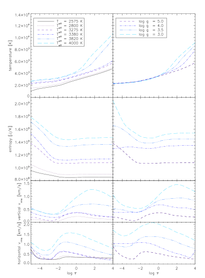
Figure 1: From top to bottom, the temperature, entropy, vertical, and horizontal velocity are plotted as a function of optical depth. The column on the left side shows models with different $T_{\mathrm{eff}}$ and constant $\log{g}$, on the right side the models are at a constant $T_{\mathrm{eff}}$ with varying $\log{g}$. The rise of horizontal velocity in the $\log{g}=4.0$ [cgs] model in the deeper atmospheric layers is due to interpolation from z- to $\tau$-scale.

3 Velocity fields in the CO⁵BOLD-models

Before we investigate the effect of velocity fields on spectral lines, we analyze the velocity fields in the models themselves and we will do this with respect to spectral lines. Spectral lines are broadened by velocity fields where the wavelength of absorption or emission of a particle is shifted due to its motion in the gas. Here we are mostly concerned with the macroscopic, hydrodynamic motions but have in mind that the thermal motions are also constituting an important contribution. If we envision each voxel in the RHD model cube to form its own spectral line, the whole line consists of a (weighted) sum of single lines. The velocity distribution might be represented by a histogram of the velocities of the voxels which gives us the velocity dispersion. We try to describe the velocity fields in that sense instead of using the rms-velocities shown in Fig.1. In the CO⁵BOLD-models, a velocity vector is assigned to each voxel and consists of the velocities in x-, y-, and z-direction. We will investigate the vertical and horizontal component of the velocity dispersion in the models and the total velocity dispersion $\sigma_{\mathrm{tot}}=\sqrt{\sigma_{x}^{2}+\sigma_{y}^{2}+\sigma_{z}^{2}}$. In order to describe the height dependent velocity dispersion we applied a binning method, i.e. we plot all velocity components of a certain horizontal plane of equal optical depth $\tau$ in the CO⁵BOLD cube in a histogram with a bin size of $25$ m s^-1.

Figure 2: Histogram of the velocity distribution in vertical direction. The normalized number of points is plotted against the vertical velocity in m/s (solid line). The Gaussian (dashed line) fits the velocity distribution and determined an FWHM value (dashed-dotted line), which is related to $\sigma$ with $FWHM=2\sqrt{\ln{2}}\cdot\sigma$. The underlying model is located at $T_{\mathrm{eff}}=2800$ K and $\log{g}=5$ [cgs].

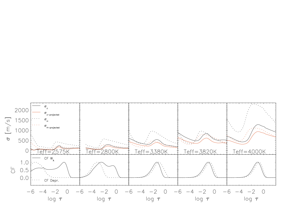
Figure 3: Upper panel: Radial ($\sigma_{z}$) and horizontal ($\sigma_{H}$) components of the velocity dispersion are plotted against the optical depth on a logarithmic scale. Bottom panel: Each bottom panel shows the contribution functions (CF) of an $\@element{\mathrm{FeH}}$-line at a wavelength of $9956.72$ $\AA$. Equivalent width $W_{\lambda}$ (solid) and the depression at the line center (dashed) of the line are plotted as a function of optical depth on a logarithmic scale. The models (from left to right) are located at $T_{\mathrm{eff}}$ of $2800$ K, $3380$ K, $3820$ K and $4000$ K and a $\log{g}$ value of $5.0$, except the one with $T_{\mathrm{eff}}\leavevmode\nobreak\ =\leavevmode\nobreak\ 3820$ K ($\log{g}\leavevmode\nobreak\ =\leavevmode\nobreak\ 4.9$), and the one with $T_{\mathrm{eff}}\leavevmode\nobreak\ =\leavevmode\nobreak\ 4000$ K ($\log{g}\leavevmode\nobreak\ =\leavevmode\nobreak\ 4.5$) [cgs].

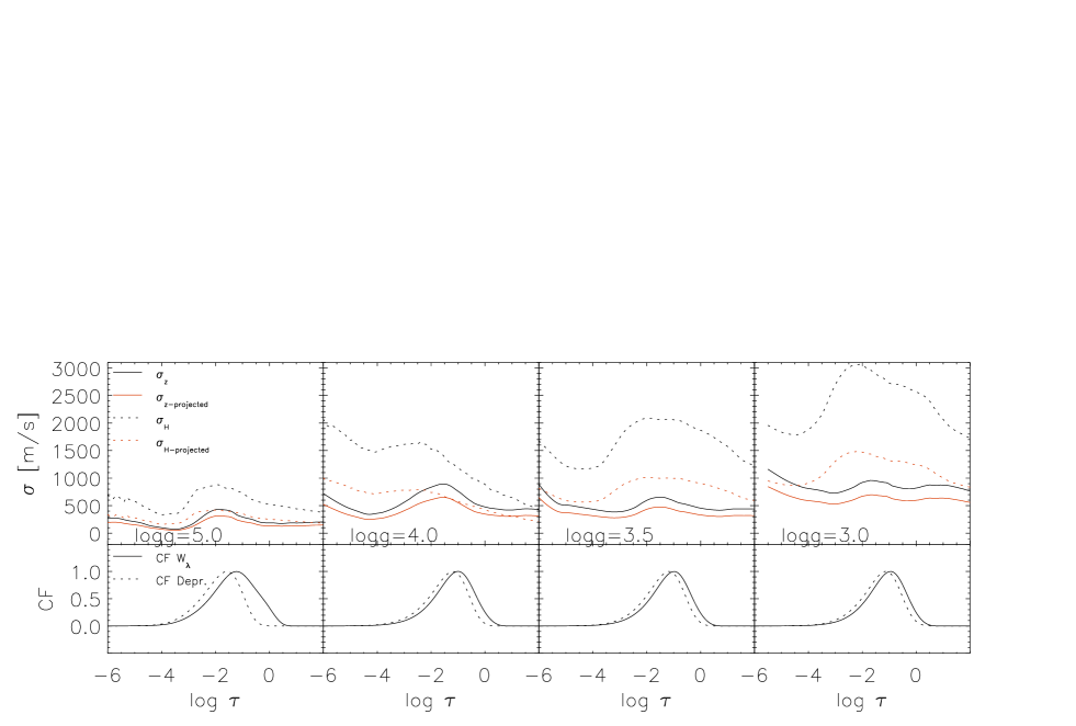
Figure 4: Upper panel: Radial ($\sigma_{z}$) and horizontal ($\sigma_{\mathrm{H}}$) components of the velocity dispersion are plotted against the optical depth on a logarithmic scale. Bottom panel: Each bottom panel shows the contribution functions (CF) of an $\@element{\mathrm{FeH}}$-line at a wavelength of $9956.72$ $\AA$. Equivalent width $W_{\lambda}$ (solid) and the depression at the line center (dashed) of the line are plotted as a function of optical depth on a logarithmic scale. The models are located at $\log{g}$ values from left to right of 5.0 ($T_{\mathrm{eff}}\leavevmode\nobreak\ =\leavevmode\nobreak\ 3275$ K), 4.0 ($T_{\mathrm{eff}}\leavevmode\nobreak\ =\leavevmode\nobreak\ 3315$ K), 3.5 ($T_{\mathrm{eff}}\leavevmode\nobreak\ =\leavevmode\nobreak\ 3270$ K) and 3.0 ($T_{\mathrm{eff}}\leavevmode\nobreak\ =\leavevmode\nobreak\ 3240$ K) [cgs].

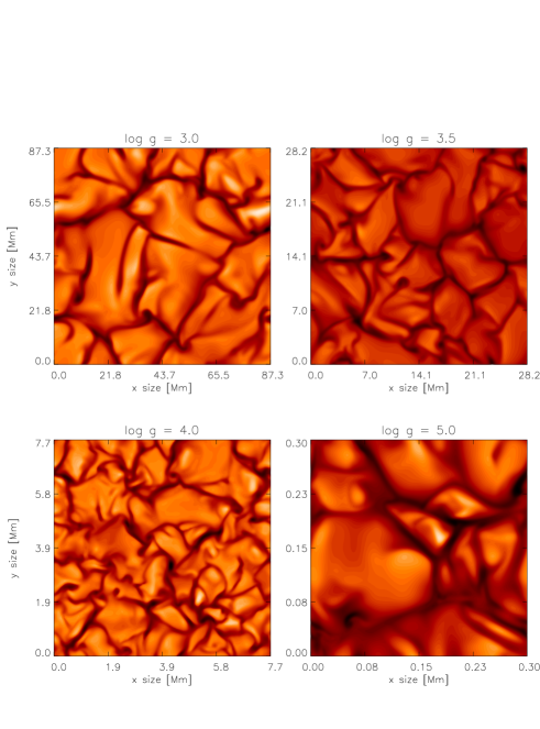
Figure 5: Horizontal cross-section around $\tau\leavevmode\nobreak\ \sim\leavevmode\nobreak\ 1$ of vertical velocity components. The models are located at $\log{g}$ values of $3.0$, $3.5$, $4.0$, and $5.0$ [cgs] (from upper left corner to lower right, respectively).

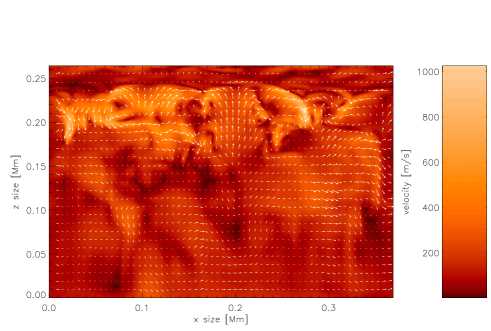
Figure 6: 2D cross-section in x-z direction of the x-z velocity in a model with $\log{g}\leavevmode\nobreak\ =\leavevmode\nobreak\ 5.0$ [cgs] and $T_{\mathrm{eff}}\leavevmode\nobreak\ =\leavevmode\nobreak\ 2800$ K. Overplotted are x-z velocity vectors. The direction of the material flow is indicated by the velocity vectors.

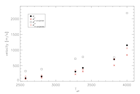
Figure 7: Plotted are the weighted projected and unprojected velocity dispersions of the horizontal and vertical component for models with different $T_{\mathrm{eff}}$. The models are located at $T_{\mathrm{eff}}$ values of $2575$ K, $2800$ K, $3275$ K, $3380$ K, $3820$ K and $4000$ K and a $\log{g}$ value of 5.0, except the one with $T_{\mathrm{eff}}\leavevmode\nobreak\ =\leavevmode\nobreak\ 3820$ K ($\log{g}\leavevmode\nobreak\ =\leavevmode\nobreak\ 4.9$), and the one with $T_{\mathrm{eff}}\leavevmode\nobreak\ =\leavevmode\nobreak\ 4000$ K ($\log{g}\leavevmode\nobreak\ =\leavevmode\nobreak\ 4.5$) [cgs].

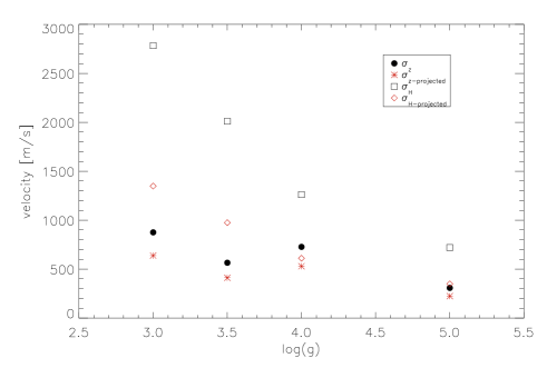
Figure 8: Plotted are the weighted projected and unprojected velocity dispersions of the horizontal and vertical component for models with different $\log{g}$. The models are located at $T_{\mathrm{eff}}$ around $3300K$ and different $\log{g}$ values of 3.0 ($T_{\mathrm{eff}}\leavevmode\nobreak\ =\leavevmode\nobreak\ 3240$ K), 3.5 ($T_{\mathrm{eff}}\leavevmode\nobreak\ =\leavevmode\nobreak\ 3270$ K), 4.0 ($T_{\mathrm{eff}}\leavevmode\nobreak\ =\leavevmode\nobreak\ 3315$ K) and 5.0 ($T_{\mathrm{eff}}\leavevmode\nobreak\ =\leavevmode\nobreak\ 3275$ K) [cgs].

We fit the histogram velocity distribution with a Gaussian normal distribution function $G=\exp{(-(\frac{x}{\sigma})^{2})}$ and take the standard deviation $\sigma$ as a measure for the velocity dispersion $\sigma$ in the models (see Fig. 2) (The relation between the Gaussian standard deviation $\sigma$ and the standard deviation $\sigma_{\mathrm{rms}}$ of the mean velocity is $\sigma=\sqrt{2}\cdot\sigma_{\mathrm{rms}}$). This is done for the $\sigma_{x}$, $\sigma_{y}$, and $\sigma_{z}$ component of the velocity vector for each horizontal plane from $\tau_{\mathrm{min}}$ to $\tau_{\mathrm{max}}$, which are the highest and the deepest points, in each model atmosphere. In this way we obtained the height dependent velocity dispersion $\sigma_{x,y,z}(\tau)$. We average over five model snapshots for a better statistical significance. In Figs. 3 and 4, the velocity dispersions for the horizontal components $\sigma_{\mathrm{H}}=\sqrt{\sigma_{x}^{2}+\sigma_{y}^{2}}$ and vertical component $\sigma_{z}$ are plotted against optical depth (black solid and dotted lines). In the latter figures, we identify the maxima around $\log{\tau}\leavevmode\nobreak\ =\leavevmode\nobreak\ -1$ of the velocity dispersions as the region where the up-flowing motion spreads out in horizontal direction and starts to fall back to deeper layers. We will call this point, the “convective turn-over point”. In a horizontal 2D cross-section of the vertical velocities, somewhat below this area, the up-flowing granulation patterns are clearly visible (see Fig.5 for models with different $\log{g}$ or Ludwig et al. (2006)). In a vertical 2D cross-section one can see the behavior of the up-streaming material (Fig. 6 shows an example for a model with $T_{\mathrm{eff}}=2800$ K). The material starts moving upwards almost coherently and before reaching higher layers (around $z\leavevmode\nobreak\ =\leavevmode\nobreak\ 200$ km in Fig. 6) of the atmosphere the vertical velocity dispersion $\sigma_{z}$ becomes maximal. After that point, the material spreads out in horizontal directions and starts falling down again. At this point, the dispersion of horizontal velocities $\sigma_{H}$ becomes maximal (convective turn-over point).

In Fig.4 we can see at lower surface gravities that the maxima of the horizontal velocity dispersion are not centered around a specified optical depth anymore; it spreads out in vertical direction and span the widest range at $\log{g}\leavevmode\nobreak\ =\leavevmode\nobreak\ 3.0$ [cgs]. The pressure stratification changes, and the convective turn-over point moves to lower gas-pressure (not shown here) but stays at almost constant optical depth between $\log{\tau}\leavevmode\nobreak\ =\leavevmode\nobreak\ 0$ and $\log{\tau}\leavevmode\nobreak\ =\leavevmode\nobreak\ -2$. With varying temperature, the position of the convective turn-over point stays at almost constant optical depth.

3.1 Reduction of the 3D velocity fields

Commonly, micro- and macro-turbulence derived from spectroscopy are interpreted as being associated with actual velocity fields present in the stellar atmosphere. In our simulations no oscillations are induced externally but small oscillations are generated in the simulations itself. The velocity amplitudes of these oscillations reach maximal $10\,\%$ of the convective velocities and have no significant influence on the macro-turbulent velocity. We would also not expect global oscillations for these objects, except for young stars with solar masses smaller than $0.1$  $M_{\bigodot}$ induced by D-burning (Palla & Baraffe, 2005). In the following, we try to make the connection between micro- and macro-turbulence and actual hydrodynamical velocity fields manifest by considering the velocity dispersion determined directly from the hydrodynamical model data, and compare it with the micro- and macro-turbulence derived from synthesized spectral lines (see Sec.3.2). This connection is algebraically not immediate, and we only apply a simple model for translating the hydrodynamical velocities into turbulent velocities relevant to spectroscopy (see appendix). When interpreting comparisons shown below the very approximate nature of our model should be kept in mind. In this model, we include the geometrical projection of the components of $\sigma_{x,y,z}$ to the line of sight of the observer. We also have to consider the effect of limb-darkening of the stellar disk. For each velocity dispersion component we calculate a projection factor which includes both, geometrical projection and limb-darkening effects (more described in the appendix). We take a limb-darkening coefficient of $0.4$ which follows from the continuum from angle dependent line synthesis performed in LINFOR3D. These simulations suggest that a linear limb-darkening law with a limb-darkening coefficient of $0.4$ is suited to describe the brightness variation. The projected velocity dispersions are also plotted in Figs. 3 and 4 (red solid and dotted lines). The reducing effect of this projection factor is stronger in the horizontal components than in the vertical because the projected area at the limb of the stellar disk, where $\sigma_{H}$ reaches its maximum value, is much smaller than in the center where $\sigma_{z}$ has its maximum value. The influence of limb-darkening is not strong and the dependence of the projection factor from the limb-darkening coefficient is only small (described in more detail in the appendix).

3.1.1 Weighted velocities

To investigate the influence of broadening from the projected and unprojected velocity dispersion on spectral lines, we use contribution functions for the equivalent width $W_{\lambda}$ and the depression at the line center of an $\@element{\mathrm{FeH}}$ line at $9956.7\leavevmode\nobreak\ \AA$ (Magain, 1986). The line gains its $W_{\lambda}$ and depression in the region between $\log{\tau}\leavevmode\nobreak\ =\leavevmode\nobreak\ 1.0$ and $\log{\tau}\leavevmode\nobreak\ =\leavevmode\nobreak\ -4.0$, i.e. that is the region of main continuum absorption caused by $\@element{\mathrm{FeH}}$ molecules. The maximum is roughly centered around $\log{\tau}\leavevmode\nobreak\ =\leavevmode\nobreak\ -1.0$ and moves to slightly lower optical depth with lower temperatures (at the lowest $T_{\mathrm{eff}}$ of $2575$ K, the maximum is centered around $\log{\tau}\leavevmode\nobreak\ =\leavevmode\nobreak\ -2.0$) or higher surface gravities. The contribution function of $W_{\lambda}$ range over the region of the convection zone and reflects its influence on the line shape. Due to the latter fact, $\@element{\mathrm{FeH}}$ lines are a good mean to explore the convective regions in M-dwarfs. In order to measure the velocities in the region where the lines originate, we compute the mean of the (projected) velocities weighted with the contribution function of $W_{\lambda}$.

$$\sigma_{\mathrm{weighted}}=\frac{\sum_{\tau=2}^{-6}\sigma_{\tau}\cdot CF_{\tau}}{\sum_{\tau=2}^{-6}CF_{\tau}}$$ (1)

The horizontal and vertical components of these weighted velocity dispersions are plotted in Figs. 7 and 8. We can see an increase of $\sigma_{H,z}$ with increasing effective temperature or decreasing surface gravity. We can see again that the projected horizontal velocity dispersions are significantly smaller than the unprojected ones due to the reasons mentioned above. The difference in the vertical component is much smaller. The velocity dispersions for the vertical component range from a few hundred m/s for cool, high gravity models to $\sim\leavevmode\nobreak\ 1$ km s^-1 for hot or low gravity models. The horizontal component range from a $\sim\leavevmode\nobreak\ 500$ m s^-1 for cool, high gravity models to $\sim\leavevmode\nobreak\ 2$ km s^-1 for hot or low gravity models. We compare the total projected velocity dispersion $\sigma_{tot}=\sqrt{\sigma_{H}^{2}+\sigma_{z}^{2}}$ in Sec. 3.2 with micro- and macro-turbulent velocities in the classical sense.

The strong increase of the velocity dispersions in the atmospheres to higher layers (Figs. 3 and 4), which some models show, is related to convective overshoot into formally stable layers. These velocities are originated by waves excited by stochastical fluid motions and by advective motions (Ludwig et al., 2002, and references therein). However, it will not affect the spectral lines, because the lines are generated in the region between an optical depth of $\log{\tau}\leavevmode\nobreak\ =\leavevmode\nobreak\ 1.0$ and $\log{\tau}\leavevmode\nobreak\ =\leavevmode\nobreak\ -4.0$. The lines on the model with $T_{\mathrm{eff}}=2575$ K are an exception, they are formed in the outermost layers of the model and it is not possible to compute the full range of formation of these lines, because the atmosphere is not extended enough. One has to keep this in mind when regarding the line dependent results of this model later in this chapter.

3.2 Radial velocity shifts

Due to the fact that in a convective motion the up-flowing area is larger, because it is hotter and less dense, than the down-flowing one, one expect a net shift of the velocity distribution to positive velocities. That means, the net amount of up-flowing area with hotter temperature, i.e. more flux in comparison to the down-flowing area, results in a blue shift in the rest wavelength position of a spectral line (see e.g. Dravins, 1982).

To see how the area of up-flowing material affects the rest wavelength position of a spectral line, we computed ten $\@element{\mathrm{FeH}}$ spectral lines (more described in Sect. 4) on 3D models to measure the displacement of the line positions. In order to determine the center of the line, we used the weighted mean $C=\frac{\sum F\cdot v}{\sum F}$ which account for the asymmetric line shape. (To use the weighted mean is appropriate here, since we have no noise in the computed data.) The line shifts of the flux and the intensity are given in Tab. 2. A negative value stands for a blue shift, and a positive for a red shift. The values for each model are the mean of five temporal snapshots. The absolute displacement of the flux and intensity in the $\log{g}$ series reflects the dependence of the velocity fields on surface gravity, but for the $T_{\mathrm{eff}}$ series a connection is barely visible (see Figs. 7 and 8). This could be due to the small geometrical size of the atmospheres in the $T_{\mathrm{eff}}$ series (see Tab. 1). Only the the one with $T_{\mathrm{eff}}=4000$ K shows a significant line shift and in this model the atmosphere is $1150$ km high due to the slightly smaller $\log{g}$ value of $4.5$ [cgs]. At this point we will not go in deeper analysis of this topic.

Since we only use five snapshots, we are dealing with statistics of small numbers and hence a big scatter in the results. This scatter $\sigma_{\mathrm{shift}}$ is in general one order lower than the shift of the line and the integrated jitter of the line, which is important for radial-velocity measurements, goes with $\sigma_{\mathrm{jitter}}=\frac{\sigma_{\mathrm{shift}}}{\sqrt{N}}$, where N is the number of snapshots. Since in a star N is of the order of $10^{6}$, the jitter will be of the order of  mm s^-1.

We did not further investigate the effect of granulation patterns on the line profiles but, as we will see below, the lines are almost Gaussian and show no direct evidence for significant granulation effects.

Table 2: Displacement $\Delta v_{\rm{Flux}}$ and $\Delta v_{\rm{Intensity}}$ in m/s of the position of an $\@element{\mathrm{FeH}}$ line from the rest wavelength on models with different $T_{\mathrm{eff}}$ (left side) and different $\log{g}$ (right side).

$T_{eff}$	$\Delta v_{\rm{Flux}}$ [m/s]	$\Delta v_{\rm{intensity}}$ [m/s]	$v_{\rm{ad}}$ [m/s]	$\log{g}$	$\Delta v_{\rm{Flux}}$ [m/s]	$\Delta v_{\rm{intensity}}$ [m/s]	$v_{\rm{ad}}$ [m/s]
2800	$0$	$2$	$3750$	3.0	$-56$	$-25$	$6100$
3275	$-1$	$3$	$4000$	3.5	$-47$	$-36$	$5500$
3380	$-2$	$2$	$4850$	4.0	$-16$	$-7$	$5400$
3820	$-1$	$-5$	$6000$	5.0	$-1$	$3$	$4500$
4000	$-44$	$-28$	$7000$

3.3 Micro- and macro-turbulent velocities

Due to the large amount of CPU-time required to compute 3D RHD models and spectral lines on these models, we want study the necessity of 3D models in the range of M-stars. Our goal is to compare the broadening effects of the 3D velocity fields on the shape of spectral lines with the broadening in terms of the classical micro- and macro-turbulence profiles (see e.g. Gray, 1977, 2008). The latter description is commonly used in 1D atmosphere models like ATLAS9 (Kurucz, 1970) or PHOENIX and related line formation codes. If the difference between 1D and 3D velocity broadening is small, the usage of fast 1D atmosphere codes to simulate M-stars for comparisons with observations, e.g. to determine rotational- or Zeeman-broadening, would be an advantage.

If the size of a turbulent element is small compared to unit optical depth, we are in the regime of the micro-turbulence. The micro-turbulent velocities might differ strongly from one position to another and have a statistical nature. The broadening effect on spectral lines can be described with a Gaussian which enters the line absorption coefficient (Gray, 2008). It can be treated similar to the thermal Doppler broadening. The effect on the shapes of saturated lines is an enhancement of line wings due to the fact that at higher velocities the absorption cross section increases and as a consequence the equivalent width ($W_{\lambda}$) of the line is increased.

If the size of a turbulent element is large compared to unit optical depth (maybe better of the same size as unit optical depth), we are in the regime of the macro-turbulence. It can be treated similar to rotational broadening as a global broadening of spectral lines. The effect is an increase of the line width but the equivalent width remains constant.

As we saw before, the velocity fields in the M-stars are not very strong in comparison to the sound speed (see Tab.2) and one could expect that their influence on line shapes do not deviate strongly from Gaussian broadening.

We compared line broadening with the radial-tangential profile from Gray (1975) and a simple Gaussian profile and found that the latter is a good approximation with an accuracy high enough for possible determination of rotational- or Zeeman-broadening. Hence, in this investigation we will assume Gaussian broadening profiles. That means, we can assume a height independent isotropic velocity distribution for micro- and macro-turbulent velocities. This is a very convenient way to simulate the velocity fields. One would expect that the anisotropic nature and the height dependence of the hydrodynamical velocity fields have a significant influence on line shapes, so it is remarkable that their influence on spectral lines can be described to a high accuracy in this way. (At least in the investigated M-type stars.) In Fig. 9, a few examples of $\left\langle\mathrm{3D}\right\rangle$-$\@element{\mathrm{FeH}}$ spectral lines were plotted, which were computed with a given micro-turbulent velocity (determined below) and then convolved with a Gaussian broadening profile with a given macro-turbulent velocity. The broadened $\left\langle\mathrm{3D}\right\rangle$-$\@element{\mathrm{FeH}}$ lines fit the 3D-$\@element{\mathrm{FeH}}$ lines very well. The difference of the 1D and 3D centroid ($C=\frac{\sum F\cdot v}{\sum F}$) range in the order of m/s for small velocity fields to $30-40$ m s^-1 for strong velocity fields in hot M star models or with low $\log{g}$. The error in flux is lower than $1\%$ (see Fig. 9) this corresponds to an uncertainty in velocity, for example rotational velocity, of less than $150$ m s^-1 depending on the position in the line. It is also visible in the latter figures that at low effective temperature effects from velocity broadening are not visible in comparison with an unbroadened $\left\langle\mathrm{3D}\right\rangle$-line in which the v.d.Waals broadening is dominant. At higher effective temperatures, the difference between broadened and unbroadened $\left\langle\mathrm{3D}\right\rangle$-lines is clearly visible. We found that in the range of M-type stars, 1D spectral synthesis of $\@element{\mathrm{FeH}}$-lines using micro- and macro-turbulent velocities in the classical description is absolutely sufficient to include the effects of the velocity fields. In the following we will determine the velocities needed.

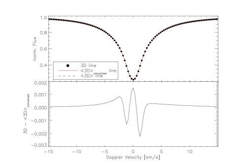
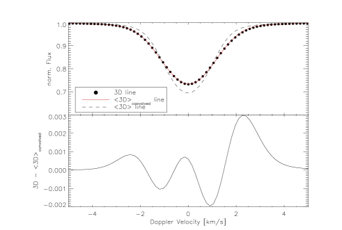
Figure 9: FeH lines for models with $T_{\mathrm{eff}}\leavevmode\nobreak\ =\leavevmode\nobreak\ 2800$ K, $\log{g}\leavevmode\nobreak\ =\leavevmode\nobreak\ 5.0$ [cgs] (top) and $T_{\mathrm{eff}}\leavevmode\nobreak\ =\leavevmode\nobreak\ 3820$ K, $\log{g}\leavevmode\nobreak\ =\leavevmode\nobreak\ 4.9$ [cgs] (bottom). The upper panels show the 3D-line (dots) and the $\left\langle\mathrm{3D}\right\rangle$_convolved-line (solid line) which was broadened by a Gaussian profile. For comparison we plotted a $\left\langle\mathrm{3D}\right\rangle$-line which was not broadened by any velocities (dashed line). In the lower panels the 3D-$\left\langle\mathrm{3D}\right\rangle$_convolved residuals are plotted. One can see the asymmetry which stems from the line shifts due to convective motions. Note the different y-axis scale.

3.3.1 Determination of micro- and macro-turbulent velocities

The investigation of the micro-turbulent velocities was done with the curve of growth (CoG) method (e.g., Gray, 2008). We artificially increase the line strength of an absorption-line (increase the $\log{gf}$ value) which in turn increase the saturation of the line and its influence of the micro-turbulent velocity, which results in an enhancement of $W_{\lambda}$. In order to determine micro-turbulent-velocities, we use Fe I- and $\@element{\mathrm{FeH}}$-lines produced on $\left\langle\mathrm{3D}\right\rangle$-models with different micro-turbulent velocities (there are no differences in micro-turbulent velocities between both types of lines), i.e. for each $\log{gf}$-value we compute a $\left\langle\mathrm{3D}\right\rangle$-line with micro-turbulent velocities between $0$ km s^-1 and $1$ km s^-1 in $0.125$ km s^-1 steps. In this way we obtained CoGs for $9$ different micro-turbulent velocities. We compare the equivalent widths in the CoGs with the ones which was computed on the 3D-models and selected the velocity of the CoG which fits the 3D CoG best in the sense of $\chi^{2}$-residuals.

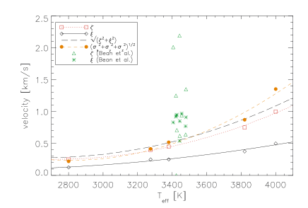
Figure 10: Macro- (solid) and micro- (dotted) turbulent velocities and the sum of both (long dashed line) as a function of $T_{\mathrm{eff}}$. The data points are fitted by a second order polynomial and the sum of micro- and macro-turbulent velocities is given by the sum of the fits. For comparison, velocities from Bean et al. and the total projected weighted 3D velocity dispersions are plotted, too (short dashed line). The models are located at $T_{\mathrm{eff}}$ values of $2800$ K, $3275$ K, $3380$ K, $3820$ K and $4000$ K and a $\log{g}$ value of 5.0, except the one with $T_{\mathrm{eff}}\leavevmode\nobreak\ =\leavevmode\nobreak\ 3820$ K ($\log{g}\leavevmode\nobreak\ =\leavevmode\nobreak\ 4.9$), and the one with $T_{\mathrm{eff}}\leavevmode\nobreak\ =\leavevmode\nobreak\ 4000$ K ($\log{g}\leavevmode\nobreak\ =\leavevmode\nobreak\ 4.5$) [cgs].

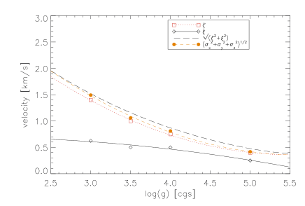
Figure 11: Macro- (solid) and micro- (dotted) turbulent velocities and the sum of both (long dashed line) as a function of $\log{g}$. The data points are fitted by a second order polynomial and the sum of micro- and macro-turbulent velocities is given by the sum of the fits. For comparison, the total projected weighted 3D velocity dispersions is plotted, too (short dashed line). The models are located at $T_{\mathrm{eff}}$ around $3300$ K and different $\log{g}$ values of 3.0 ($T_{\mathrm{eff}}\leavevmode\nobreak\ =\leavevmode\nobreak\ 3240$ K), 3.5 ($T_{\mathrm{eff}}\leavevmode\nobreak\ =\leavevmode\nobreak\ 3270$ K), 4.0 ($T_{\mathrm{eff}}\leavevmode\nobreak\ =\leavevmode\nobreak\ 3315$ K) and 5.0 ($T_{\mathrm{eff}}\leavevmode\nobreak\ =\leavevmode\nobreak\ 3275$ K) [cgs].

The macro-turbulent velocities are determined by computing a $\left\langle\mathrm{3D}\right\rangle$-model $\@element{\mathrm{FeH}}$ line (at $\lambda=9956.7\leavevmode\nobreak\ \AA$) including the micro-turbulent velocities. This line is then broadened with a Gaussian profile and different velocities until it matches the 3D-model line.

The dependence of the micro- ($\xi$) and macro- ($\zeta$) turbulent velocities on surface gravity and effective temperature is plotted in Figs. 10 and 11. The macro-turbulent velocities in both cases show a quadratic dependence, and we can fit them with a second order polynomial. The micro-turbulent velocities could be fitted by a linear function or a second order polynomial. We decided to use the second order polynomial, too.

Micro- and macro-turbulence velocities both show a similar dependence on surface gravity and effective temperature, which implies that there is a direct connection between both. A comparison of the macro ($\zeta$)- and micro ($\xi$)-turbulent velocities with the sum of both ($\sqrt{\zeta^{2}+\xi^{2}}$) and the total projected weighted velocity dispersion $\sigma_{\mathrm{tot}}$ (see Sec. 3) is also shown in Figs. 10 and 11. The total projected weighted velocity dispersion (see Sec.3) is very similar to the macro-turbulent velocities and in most cases smaller than the sum of micro- and macro-turbulent velocity. It is remarkably, that it is possible, with this simple description of the total projected weighted velocity, to describe the broadening influence of the hydrodynamical velocity fields on spectral lines in comparison with the classical micro- and macro-turbulent description.

In order to obtain a good estimate of the line profile in 1D spectral line synthesis, knowledge of the micro- and macro-turbulent velocities is very important. Otherwise one could underestimate the equivalent width or the line width and hence obtain a wrong line depth.

We compare our micro- and macro-turbulent velocities to observational results from (see Bean et al., 2006a, b; Bean, 2007). Our value of the macro-turbulent velocities are roughly of the same order. The higher macro-turbulent velocities from Bean et al. possibly contain rotational broadening, but the Bean et al. micro-turbulent velocities are roughly a factor two or three higher than ours. These velocities are obtained from observed spectra by the authors of the afore-mentioned papers using spectral fitting procedures. In detail, they used PHOENIX atmosphere models and the stellar analysis code MOOG (Sneden, 1973). One has to keep in mind that the empirical determination of micro-turbulence is also endangered to suffer from systematic errors. For most of the lines that Bean and collaborators employ (line data from Barklem et al. (2000)), the v.d.Waals damping constant is available. However, in some cases not, then usually Unsöld’s hydrogenic approximation is applied to calculate the value, and different authors use significantly different enhancement factors changing its value. This illustrates the level of uncertainty inherent to this approach. For instance, Schweitzer et al. (1996) use an enhance factor of 5.3 (for the resulting $\gamma_{6}$ values) for their Fe I lines, while Bean et al. prefer 2.5 for Ti I lines (Bean, 2007). To investigate the detailed influence of v.d.Waals broadening on determination of micro-turbulence velocities is very interesting, but goes beyond the scope of this paper. We want to point out, that it is perceivable that uncertainties in the damping constant can introduce significant systematic biases in the resulting value of spectroscopically micro- and macro-turbulence and they could easily be overestimated.

As mentioned above and illustrated Fig. 10, our prediction of the micro-turbulence grossly underestimates the micro-turbulence values measured by Bean et al.. This might hint at deficits in the hydrodynamical modeling and we cannot exclude the possibility that a process is missing in our 3D models leading to a substantially higher micro-turbulence. But due to the argumentation above and a comparison with the solar micro- and macro-turbulence, we argue that the Bean et al. values for the micro-turbulence are too high. However, before being able to draw definite conclusions the observational basis has to be enlarged.

4 $T_{\mathrm{eff}}$- and $\log{g}$-dependence of $\@element{\mathrm{FeH}}$ molecular lines

In this section we study the dependence of $\@element{\mathrm{FeH}}$ molecular lines on $T_{\mathrm{eff}}$ and $\log{g}$ in our 3D- and $\left\langle\mathrm{3D}\right\rangle$-models. Again, the intention is to identify multi-D effects which might hamper the use of the $\@element{\mathrm{FeH}}$ line diagnostics in standard 1D analyses. For this purpose we compute the $\left\langle\mathrm{3D}\right\rangle$-lines with no micro- and macro-turbulence velocity. With this method we can study the $\@element{\mathrm{FeH}}$ lines without any velocity effects and can through direct comparison between 3D- and $\left\langle\mathrm{3D}\right\rangle$-lines clearly identify velocity induced effects.

4.1 $\@element{\mathrm{FeH}}$ line data

Wing & Ford (1969) were the first to detect a broad molecular absorption band around $991$ nm in late M dwarfs. This band was later found in S stars (Wing, 1972) and in sun spots. Nordh et al. (1977) identified the Wing-Ford band as the $0-0$ band of a $\@element{\mathrm{FeH}}$ electronic transition. The $\@element{\mathrm{FeH}}$ molecule is well suited for the measurements mentioned in the introduction because of its intrinsically narrow and well isolated spectral lines. These lines are also an ideal tracer of line broadening in M-stars due to convection or very slow rotation (Reiners, 2007). Since $\@element{\mathrm{FeH}}$ lines were not very commonly used for the interpretation of stellar spectra in the past, only little data is recorded in the literature. With the work of Dulick et al. (2003), it is possible to determine the $\log{gf}$ value and the transition energies. For the partition function, a combination of the tabulated function in Dulick et al. (2003) and an analytically determined one from the Eq.$1$ in Sauval & Tatum (1984) is used.

Due to the high atmospheric pressures, v.d.Waals broadening is often significant in cool M-type dwarfs. No detailed calculations exist for the v.d.Waals broadening of $\@element{\mathrm{FeH}}$ molecular lines. Lacking a more accurate treatment, we follow the approximate approach of Schweitzer et al. (1996) and apply Unsöld’s hydrogenic approximation, albeit – different from Schweitzer and co-workers – we do not apply an enhancement factor to the calculated broadening constant $C_{6}$.

The ionization energy of the $\@element{\mathrm{FeH}}$ molecule enters the calculation of $C_{6}$ which, unfortunately, is not known. Only the dissociation energy is published of $1.59\pm 0.08$ eV at 0 K (e.g. Dulick et al., 2003). To derive an estimate of the ionization energy, we heuristically compare the ionization and dissociation energies of a large number of hydrides taking data from Wilkinson (1963). We find an approximately linear relationship between the ionization and the dissociation energies of hydrides. For $\@element{\mathrm{FeH}}$ we obtain an ionization energy of $6$ eV for the known dissociation energy from a linear fit. Computation of this value from the ionization-potential of Fe and the dissociation energies of $\@element{\mathrm{FeH}}$ and $\@element{\mathrm{FeH}}$⁺ yields $7.3$ eV (Bernath 2008, private communication), which is compatible with our value considering our rather crude procedure. The difference in FWHM of synthesized $\@element{\mathrm{FeH}}$-lines in the range between 6 and $7.3$ eV amounts to $\approx 25$ m/s. This uncertainty is quite acceptable in comparison to the total broadening of typically several 100 m s^-1 in this investigation.

4.2 An ensemble of 3D- and $\left\langle\mathrm{3D}\right\rangle$-$\@element{\mathrm{FeH}}$ lines

We investigate ten $\@element{\mathrm{FeH}}$ lines between $9950$ Å and $9990$ Å chosen from Reiners & Basri (2006) (see Tab. 3). We choose lines from different branches (Br), orbital angular momentum $\omega$, and rotational quantum number $J$. The wavelengths in Tab. 3 are given in vacuum and $E_{l}$ is the lower transition energy. While not directly relevant in the present context, because we do not study the effects of magnetic fields, we note that five lines are magnetically sensitive and five insensitive. We performed the line synthesis for fixed abundances on the CO⁵BOLD atmosphere models listed in Tab. 1. The spectral resolution is $R\leavevmode\nobreak\ \approx\leavevmode\nobreak\ 2\cdot 10^{6}$ ($\equiv 5\cdot 10^{-3}$ Å) corresponding to a Doppler velocity of $v\leavevmode\nobreak\ \approx\leavevmode\nobreak\ 150$ m s^-1 at the wavelength of the considered lines ($\sim\leavevmode\nobreak\ 9950\leavevmode\nobreak\ \AA$). Figures 12 and 13 illustrate the strong influence of surface gravity and effective temperature on the line shape for the 3D-models. In Fig. 12, one can see that for both, $\left\langle\mathrm{3D}\right\rangle$- and 3D-lines, the line depth, line width and equivalent width $W_{\lambda}$ decrease strongly with increasing effective temperature. The decrease of $W_{\lambda}$ is due to stronger dissociation of the $\@element{\mathrm{FeH}}$ molecules at higher temperatures, i.e the number of $\@element{\mathrm{FeH}}$ molecule absorber decreases. Differences in the line shape between 3D- and $\left\langle\mathrm{3D}\right\rangle$-lines with changing temperature are hardly visible. To higher $T_{\mathrm{eff}}$ values, the influence of broadening on the 3D lines due to velocity fields is slightly visible and not covered by thermal and v.d.Waals broadening anymore. To cooler temperatures, the velocity fields decrease and the differences between the $\left\langle\mathrm{3D}\right\rangle$- and 3D-line shapes vanishes. The v.d.Waals broadening is larger then the thermal broadening or that from the small velocity fields in the RHD models. In the model with $T_{\mathrm{eff}}\leavevmode\nobreak\ =\leavevmode\nobreak\ 2800$ K, the lines start to become saturated. The $\@element{\mathrm{FeH}}$ lines in the z-band at effective temperatures below $\sim\leavevmode\nobreak\ 2600$ K become too saturated and too broad for investigations of quantities like magnetic field strength or rotational broadening below $10$ km s^-1.

The differences between 3D- and $\left\langle\mathrm{3D}\right\rangle$-line shapes of the $\log{g}$-series in Fig. 13 is more obvious than in the $T_{\mathrm{eff}}$ case. The differences in line depth and line width become significant with decreasing $\log{g}$. The lines in the 3D-models are significantly broadened due to the velocity fields in the RHD models, hence the line width is larger and the line depth lower. As we saw in Chapter 3, these velocity fields increase with decreasing $\log{g}$ and could be described in the 1D case in terms of macro- and micro-turbulent velocities.

The $\left\langle\mathrm{3D}\right\rangle$-lines become slightly shallower and narrower towards smaller $\log{g}$. The equivalent width of the lines decreases with decreasing $\log{g}$ due to decreasing pressure and hence decreasing concentration of of $\@element{\mathrm{FeH}}$ molecules. Also the v.d.Waals broadening looses its influence to lower pressures and the line width decreases. We point out, that we use in all models the same solar like chemical compositions, hence the concentration of $\@element{\mathrm{Fe}}$ and $\@element{\mathrm{H}}$ stays the same. The creation of $\@element{\mathrm{FeH}}$ also depends on the number of H₂-molecules, which become larger towards lower temperatures and will be important in cool models.

The slightly different effective temperatures in the models with different $\log{g}$ (see Tab. 1) affect the line depths as well. If the effective temperatures would be the same in the $\log{g}$-models, one could expect a monotonic behavior in decreasing line strength for decreasing surface gravity in the $\left\langle\mathrm{3D}\right\rangle$-lines. However, because the model with $\log{g}\leavevmode\nobreak\ =\leavevmode\nobreak\ 3.0$ is cooler, the line depth is deeper than that of the one with $\log{g}\leavevmode\nobreak\ =\leavevmode\nobreak\ 3.5$. In the following analysis we will correct the FWHM, $W_{\lambda}$, and the line depth of the lines on models with different $\log{g}$ for their slightly different effective temperatures.

The ten $\@element{\mathrm{FeH}}$ lines behave all in the same way as the presented ones. We do not see any effect of different excitation potentials or $\log{gf}$ values in the line shapes that cannot be explained by their different height of formation. Thus, we expect that we can exclude an extraordinary interaction between these quantities and effective temperature or surface gravity. We will quantify this preliminary result in the next section.

Table 3: Several quantities of the investigated $\@element{\mathrm{FeH}}$ lines (Reiners & Basri, 2006).

$\lambda_{rest}$ [Å]	$\log{gf}$	$E_{l}$ [eV]	$Br.$	$J$	$\Omega$	$magn.\leavevmode\nobreak\ sen.$
9953.08	-0.809	0.156	R	10.5	1.5	weak
9954.00	-2.046	0.199	P	16.5	2.5-3.5	strong
9956.72	-0.484	0.375	R	22.5	3.5	strong
9957.32	-0.731	0.194	R	12.5	1.5	weak
9973.80	-0.730	0.196	R	12.5	1.5	weak
9974.46	-1.164	0.108	R	4.5	0.5	weak
9978.22	-1.190	0.030	Q	2.5	2.5	strong
9979.14	-1.411	0.093	R	2.5	0.5	strong
9981.46	-1.006	0.130	R	6.5	0.5	weak
9982.60	-1.322	0.035	Q	3.5	2.5	strong

Figure 12: $\@element{\mathrm{FeH}}$ lines with constant $\log{g}$ and varying $T_{\mathrm{eff}}$. Plotted are pairs of 3D- and $\left\langle\mathrm{3D}\right\rangle$-lines shifted by a constant for better visibility. The models are located at $T_{\mathrm{eff}}$ values of $2800$ K, $3275$ K, $3380$ K, $3820$ K and $4000$ K and a $\log{g}$ value of 5.0, except the one with $T_{\mathrm{eff}}\leavevmode\nobreak\ =\leavevmode\nobreak\ 3820$ K ($\log{g}\leavevmode\nobreak\ =\leavevmode\nobreak\ 4.9$), and the one with $T_{\mathrm{eff}}\leavevmode\nobreak\ =\leavevmode\nobreak\ 4000$ K ($\log{g}\leavevmode\nobreak\ =\leavevmode\nobreak\ 4.5$) [cgs].

Figure 13: $\@element{\mathrm{FeH}}$ lines wit constant $T_{\mathrm{eff}}$ and varying $\log{g}$. Plotted are pairs of 3D- and $\left\langle\mathrm{3D}\right\rangle$-lines shifted by a constant for better visibility. The models are located at a $T_{\mathrm{eff}}$ around $3300K$ and different $\log{g}$ values of 3.0 ($T_{\mathrm{eff}}\leavevmode\nobreak\ =\leavevmode\nobreak\ 3240$ K), 3.5 ($T_{\mathrm{eff}}\leavevmode\nobreak\ =\leavevmode\nobreak\ 3270$ K), 4.0 ($T_{\mathrm{eff}}\leavevmode\nobreak\ =\leavevmode\nobreak\ 3315$ K) and 5.0 ($T_{\mathrm{eff}}\leavevmode\nobreak\ =\leavevmode\nobreak\ 3275$ K) [cgs]. The large differences between 3D- and $\left\langle\mathrm{3D}\right\rangle$-lines stem from the hydrodynamical velocity fields in the 3D models.

4.3 $\@element{\mathrm{FeH}}$ Line shapes

To quantify the visual results of Fig. 12 and Fig. 13, we measured $W_{\lambda}$, the FWHM, and the line depth of the ten investigated $\@element{\mathrm{FeH}}$-lines (see Tab. 3). We compare 3D- and $\left\langle\mathrm{3D}\right\rangle$-lines with each other to study the effects of the velocity fields in the 3D models and to explore the behavior of the $\@element{\mathrm{FeH}}$ without broadening effects from the hydrodynamical motions. A run of these quantities is plotted in Fig. 14 and Fig. 15.

As we mentioned above, we have to correct the line quantities from models with changing $\log{g}$ for their slightly different $T_{\mathrm{eff}}$. In Figs. 12 and 14 one can see how the investigated quantities depend on $T_{\mathrm{eff}}$. We determined spline fits $\wp$ for the three quantities of each line. For these fitting functions $\wp$ we took into account all five different effective temperatures. In order to correct the line quantities to a reference temperature of $T_{\mathrm{eff}}^{\mathrm{Ref.}}=3275$ K, we use a correction factor $\gamma=\frac{\wp_{\mathrm{quant.}}(T_{\mathrm{eff}}^{\mathrm{Ref.}})}{\wp_{\mathrm{quant.}}(T_{\mathrm{eff}}.)}$ and multiply the quantity for the $\log{g}$-model with $\gamma$. This gives us the value of the quantity for a $\log{g}$-model which would have $T_{\mathrm{eff}}=3275$ K.

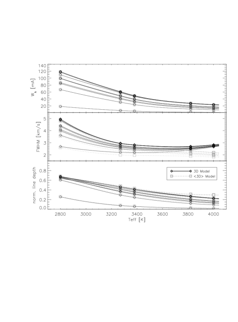
Figure 14: Run of $W_{\lambda}$ (top), FWHM (middle) and the line depth (bottom) of ten $\@element{\mathrm{FeH}}$-lines (see Tab. 3) on models with different $T_{\mathrm{eff}}$. Squares are the data points for the $\left\langle\mathrm{3D}\right\rangle$-models and diamonds for the 3D-models. $W_{\lambda}$ and FWHM are on a logarithmic ordinate for better visibility. We connect the data points of each line with fitting functions (see text) to guide the eye. Plotted are the quantities of the 3D-models (black solid lines) and the $\left\langle\mathrm{3D}\right\rangle$-models (gray dotted lines). The models are located at $T_{\mathrm{eff}}$ values of $2800$ K, $3275$ K, $3380$ K, $3820$ K and $4000$ K and a $\log{g}$ value of 5.0, except the one with $T_{\mathrm{eff}}\leavevmode\nobreak\ =\leavevmode\nobreak\ 3820$ K ($\log{g}\leavevmode\nobreak\ =\leavevmode\nobreak\ 4.9$), and the one with $T_{\mathrm{eff}}\leavevmode\nobreak\ =\leavevmode\nobreak\ 4000$ K ($\log{g}\leavevmode\nobreak\ =\leavevmode\nobreak\ 4.5$) [cgs].

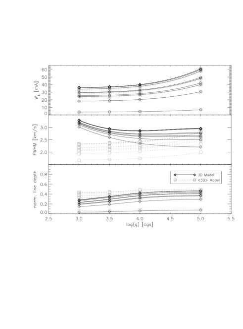
Figure 15: Run of $W_{\lambda}$ (top), FWHM (middle) and line depth (bottom) of ten $\@element{\mathrm{FeH}}$-lines (see Tab. 3) on models with different $\log{g}$. Squares are the data points for the $\left\langle\mathrm{3D}\right\rangle$-models and diamonds for the 3D-models. We connect the data points of each line with fitting functions (see text) to guide the eye. Plotted are the quantities of the 3D-models (black solid lines) and the $\left\langle\mathrm{3D}\right\rangle$-models (gray dotted lines). All quantities are corrected to a $T_{\mathrm{eff}}$ of $3275$ K.

Figure 16: 3D – $\left\langle\mathrm{3D}\right\rangle$ corrections to $\@element{\mathrm{FeH}}$ abundances derived from different $\@element{\mathrm{FeH}}$ lines with varying quantities see Tab. 3. Upper panel: The models are located at a $T_{\mathrm{eff}}$ around $3300K$ and different $\log{g}$ values of 3.0 ($T_{\mathrm{eff}}\leavevmode\nobreak\ =\leavevmode\nobreak\ 3240$ K), 3.5 ($T_{\mathrm{eff}}\leavevmode\nobreak\ =\leavevmode\nobreak\ 3270$ K), 4.0 ($T_{\mathrm{eff}}\leavevmode\nobreak\ =\leavevmode\nobreak\ 3315$ K) and 5.0 ($T_{\mathrm{eff}}\leavevmode\nobreak\ =\leavevmode\nobreak\ 3275$ K) [cgs]. Lower panel: The models are located at $T_{\mathrm{eff}}$ values of $2800$ K, $3275$ K, $3380$ K, $3820$ K and $4000$ K and a $\log{g}$ value of 5.0, except the one with $T_{\mathrm{eff}}\leavevmode\nobreak\ =\leavevmode\nobreak\ 3820$ K ($\log{g}\leavevmode\nobreak\ =\leavevmode\nobreak\ 4.9$), and the one with $T_{\mathrm{eff}}\leavevmode\nobreak\ =\leavevmode\nobreak\ 4000$ K ($\log{g}\leavevmode\nobreak\ =\leavevmode\nobreak\ 4.5$) [cgs].

4.3.1 Equivalent Width $W_{\lambda}$

In the $T_{\mathrm{eff}}$-series, $W_{\lambda}$ (see Fig. 14 upper panel) decreases with increasing $T_{\mathrm{eff}}$. At higher $T_{\mathrm{eff}}$ the number of $\@element{\mathrm{FeH}}$ molecules decrease due to dissociation and hence $W_{\lambda}$. This can be seen in the 3D lines as well as in the $\left\langle\mathrm{3D}\right\rangle$-lines. At $T_{\mathrm{eff}}=2800$ K, the influence of v.d.Waals broadening in the 3D- and $\left\langle\mathrm{3D}\right\rangle$-lines becomes clearly visible in the line profile due to saturation of the $\@element{\mathrm{FeH}}$ lines. The ten different $\@element{\mathrm{FeH}}$ lines all behave in a similar manner. The only difference is the absolute value of $W_{\lambda}$, which depends on the $\log{gf}$-value and excitation potential $E_{l}$ of each line.

In the $\log{g}$-series, the $W_{\lambda}$ (see Fig. 15 upper panel) increases with increasing $\log{g}$. The change in concentration of $\@element{\mathrm{FeH}}$ with lower $\log{g}$, which results in smaller $W_{\lambda}$, depends on the changing pressure and density stratification. The difference between 3D- and $\left\langle\mathrm{3D}\right\rangle$-lines at small $\log{g}$-values stems from the broadening by micro-turbulent velocities and vanishes to higher $\log{g}$ values. This time the $\@element{\mathrm{FeH}}$ lines are only mildly saturated, but the velocity fields in the RHD models (see Sec.3) are strong enough to affect the $W_{\lambda}$ as well. Like in the $T_{\mathrm{eff}}$-series, the ten different lines show no significant variations in their behavior. They only vary in the amount of $W_{\lambda}$ due to different $\log{gf}$-values.

Since the differences in $W_{\lambda}$ are very small, one can expect that the 3D correction to the $\@element{\mathrm{FeH}}$ abundance is very small too. We derive abundance corrections from comparison between 3D and $\left\langle\mathrm{3D}\right\rangle$ curve of growths for each set of lines on the different model atmospheres. The results are plotted in Fig. 16. In this case the correction to the different $T_{\mathrm{eff}}$ of the $\log{g}$ models is not applied. The 3D-$\left\langle\mathrm{3D}\right\rangle$ abundance correction is between $-0.001$ dex for the coolest high $\log{g}$ model and $-0.07$ dex for the $\log{g}=3.0$ model. In all cases the abundance correction is negative which mean that the 3D lines appear stronger due to the enhanced opacity which becomes larger due to the micro-turbulent velocity.

4.3.2 FWHM

The dependence of the line width (measured as the width of the line at their half maximum (FWHM)) on $T_{\mathrm{eff}}$ is shown in the middle panel of Fig. 14. At low $T_{\mathrm{eff}}$, one can see that the FWHM of the 3D- and $\left\langle\mathrm{3D}\right\rangle$-$\@element{\mathrm{FeH}}$ lines decreases with increasing $T_{\mathrm{eff}}$. The v.d.Waals broadening loses influence and also the dissociation of $\@element{\mathrm{FeH}}$ molecules leads to smaller and narrower lines. After $T_{\mathrm{eff}}$ around $3380$ K, the FWHM of the 3D lines reaches a flat minimum and starts to become larger again to higher $T_{\mathrm{eff}}$. This rise in the line width is probably related to the rising velocity fields in the RHD models, since thermal broadening takes place in both, 3D- and $\left\langle\mathrm{3D}\right\rangle$-lines and the latter still decrease. The rise of the velocity in the models with a $T_{\mathrm{eff}}$ of $3380$ K and $4000$ K could also be due to the slightly lower surface gravity in these models, but we think that the main influence stems from the higher temperatures. The $\left\langle\mathrm{3D}\right\rangle$-lines decrease monotonically with increasing $T_{\mathrm{eff}}$ and reflects the behavior of $W_{\lambda}$. The difference in FWHM between 3D- and $\left\langle\mathrm{3D}\right\rangle$-lines is very small at $T_{\mathrm{eff}}=2800$ K and increases with increasing $T_{\mathrm{eff}}$ to $\sim\leavevmode\nobreak\ 0.8$ km s^-1 at the highest $T_{\mathrm{eff}}$. We have seen in Sec.3.2 that this can be explained with the micro- and macro-turbulence description. The offset between the FWHM of the ten lines is due to their different $\log{gf}$-values i.e. large $\log{gf}$-values results in large FWHM. But since we are interested in broadening from the velocity fields, we have to take into account that lines with small $\log{gf}$-values, i.e. weak lines, formed deeper in the atmosphere where the convective motions are stronger. These lines are more broadened from the hydrodynamical velocity fields and hence more widened. We can see in Fig. 14 that the difference in FWHM between the ten 3D lines becomes smaller to high $T_{\mathrm{eff}}$. This is also valid for the lines in the $\log{g}$-series where the difference in FWHM between the ten 3D lines becomes smaller to small $\log{g}$-values.

In the $\log{g}$-series, the dependence of FWHM (Fig. 15 middle panel) is very different for 3D- and $\left\langle\mathrm{3D}\right\rangle$-lines. In the 3D case the FWHM stays almost constant with decreasing surface gravity between $\log{g}$ of $5.0$ and $4.0$ for most lines. This is due to the smaller amount of v.d.Waals broadening, which loses its influence due to lower pressure in models with smaller surface gravity. This is compared from the broadening due to the rising velocity fields. With $\log{g}$ smaller than $4.0$, the width starts to increase for all lines. This increase of line width in the 3D case is a consequence of the hydrodynamic velocity fields which increase strongly with decreasing $\log{g}$. In the $\left\langle\mathrm{3D}\right\rangle$ case, without the velocity fields, the FWHM decreases with decreasing surface gravity and reflects the behavior of the $W_{\lambda}$. The difference between 3D- and $\left\langle\mathrm{3D}\right\rangle$-lines reach its maximal value at $\log{g}=3.0$ [cgs] and is around $1.3$ km s^-1. This is on the order of the velocity fields in the RHD models (see Fig. 8). One could fit 1D spectral synthesis $\@element{\mathrm{FeH}}$ lines to observed ones (with known $T_{\mathrm{eff}}$) with the micro- and macro-turbulence description (see Sec. 3.2) and it will be possible with the obtained velocities to determine a surface gravity with the help of Fig. 11.

We did not see any significant different behavior between the ten $\@element{\mathrm{FeH}}$ lines. Neither in the $T_{\mathrm{eff}}$-series nor in the $\log{g}$-series.

4.3.3 Line Depth

In the bottom panel of Fig. 14 one can see the dependence of the line depth on $T_{\mathrm{eff}}$. The line depth increases with decreasing $T_{\mathrm{eff}}$, and almost all $\@element{\mathrm{FeH}}$ lines, except the one with the lowest $\log{gf}$ values are saturated at $T_{\mathrm{eff}}=2800$ K. The difference in line depth between 3D and $\left\langle\mathrm{3D}\right\rangle$-lines is changing in the $T_{\mathrm{eff}}$-interval. At high $T_{\mathrm{eff}}$, the line depth of the $\left\langle\mathrm{3D}\right\rangle$-lines is deeper than that of the 3D lines. At $T_{\mathrm{eff}}=2800$ K, this difference almost vanishes. This behavior is due to the saturation of the $\@element{\mathrm{FeH}}$ lines at low $T_{\mathrm{eff}}$ because both, the 3D- and $\left\langle\mathrm{3D}\right\rangle$-lines reach their maximal depth. The decrease of the line depth with increasing $T_{\mathrm{eff}}$ is due to the dissociation of the $\@element{\mathrm{FeH}}$ molecules at higher temperatures.

The line depth of the $\log{g}$-series is shown in the bottom panel of Fig. 15. At low $\log{g}$, the line depths of the 3D and $\left\langle\mathrm{3D}\right\rangle$-lines increase almost linearly with increasing $\log{g}$. The 3D lines increase with a strong slope and the $\left\langle\mathrm{3D}\right\rangle$-lines with a weaker slope. The difference in line depth between 3D- and $\left\langle\mathrm{3D}\right\rangle$-models is maximal at $\log{g}=3.0$ [cgs] and vanishes almost at $\log{g}=5.0$ [cgs]. It is consistent with the velocity fields present in the atmospheres of the RHD models broadening the lines and lower the line strength of the 3D lines. The $\left\langle\mathrm{3D}\right\rangle$-lines reflect the decreasing number of $\@element{\mathrm{FeH}}$ molecules with decreasing $\log{g}$ due to the lower pressures.

5 Summary and Conclusion

We investigated a set of M-star models with $T_{\mathrm{eff}}=2500$ K - $4000$ K and $\log{g}=3.0$ – $5.0$ [cgs]. For these models, the 3D hydrodynamic radiative transfer code CO⁵BOLD was used. The horizontal and vertical velocity fields in the 3D models were described with a binning method. The convective turn-over point is clearly visible in the atmospheric velocity dispersion structure. To investigate the influence of these velocity fields on spectral line shapes, a description for geometrical projection and limb-darkening effects was applied. With the use of contribution functions, we took only these parts in the atmosphere into account where the lines were formed. The resulting velocity dispersions range from $400$ – $1600$ m s^-1 with decreasing $\log{g}$ and with increasing $T_{\mathrm{eff}}$ from $200$ – $1400$ m s^-1. These values agree well with velocities deduced from line shapes. We expressed the hydrodynamical velocity fields of the 3D models in terms of the classical micro- and macro-turbulent velocities. With this description and the obtained micro- and macro-turbulent velocities, it is possible to reproduce 3D spectral lines on 1D atmosphere models very accurately, hence time consuming 3D treatment of $\@element{\mathrm{FeH}}$ molecular lines in the regime of cool stars is not necessary for line profile analysis. A comparison of our velocities with a set of velocities determined from observations with spectral fitting methods showed that the macro-turbulent velocities agree, but the micro-turbulent velocities are a factor of two or three smaller than the ones determined from observations.

A line shift due to the larger up-flowing area in the convection zone was investigated too. It is on the order of a few m/s up to $50$ m s^-1 for a very low gravity model. The time dependent jitter in line positions is only about m/s and would be reduced to  mm s^-1 in a real star, due to high number of contributing elements.

In order to use $\@element{\mathrm{FeH}}$ molecular lines for investigations of spectroscopic/physical properties in cool stars (e.g. Zeeman- or rotational broadening), we explored the behavior in a set of lines on $\log{g}$ and $T_{\mathrm{eff}}$. We investigated ten $\@element{\mathrm{FeH}}$ lines between 9950Å and 9990Å on our models with the spectral synthesis code LINFOR3D. $\@element{\mathrm{FeH}}$ lines react on different effective temperatures as expected due to the change in chemical composition and pressure. The lines showed also a weak dependence on surface gravity due to changing densities and pressure. The broadening from velocity fields in the 3D models of the $\log{g}$ series is very strong, but for the $T_{\mathrm{eff}}$ series the broadening from velocity fields is almost covered by v.d.Waals broadening. The difference in line width for hot models is up to $0.5$ km s^-1 and for low gravity models around $1$ km s^-1. That means for the 1D spectral synthesis, that one has to include correct micro- and macro-turbulent velocities for small surface gravities or hot $T_{\mathrm{eff}}$. Due to the fact that the FWHM $\log{g}$ dependence of $\@element{\mathrm{FeH}}$ lines goes in the opposite direction as the $\log{g}$ dependence of the velocity fields, the $\@element{\mathrm{FeH}}$ lines become a great mean to measure surface gravities in cool stars. Because the velocity fields scale with $\log{g}$ and it should be easily possible to detect them.

$\@element{\mathrm{FeH}}$ lines with different quantum numbers do not show significant differences for both, $\log{g}$- and $T_{\mathrm{eff}}$-series. That means the broadening of the lines does not depend on $J$, $\Omega$, or the branch. Furthermore lines with weak magnetic sensitivity behave just like lines with strong magnetic sensitivity. All lines are broadened in the same way by thermal and hydrodynamical motions. Only the transition probability expressed in the $\log{gf}$ value influences the behavior of the lines. The line with the lowest $gf$-values did not saturate at low $T_{\mathrm{eff}}$, but in general they are similar to the other $\@element{\mathrm{FeH}}$ lines.

It is possible to treat the $\@element{\mathrm{FeH}}$ molecular lines with different quantum numbers as homogenous in the absence of magnetic fields. That allows to use $\@element{\mathrm{FeH}}$ lines to measure magnetic fields (Reiners & Basri, 2006, 2007). Hence we conclude, that these lines also are an appropriate mean to measure magnetic field strength in M-type stars.

Appendix

Figure 17: Projection factors (vertical solid line and horizontal dotted line) as a function of the limb darkening coefficient $\epsilon$.

To compare the hydrodynamical velocity dispersion in 3D-CO⁵BOLD models with the spectroscopic quantities micro- and macro-turbulent velocities, we assume a simple geometrical model and try to resample the broadening of absorption lines. An intensity beam “sees” the velocity field under a certain angle and the spectral line is broadened by the projection of these velocities. In this sense we project the geometrical velocity components on a line of sight under a certain angle and integrate over all angles in a half sphere. We also take a linear limb-darkening law into account. We assume a velocity function $f(v)$ in velocity space and an intensity line profile

$$I(v)=V(v)\cdot I_{c}^{0}\cdot L(\theta),$$ (2)

where $V(v)$ is a line profile function, $I_{c}^{0}$ the continuum intensity at the center of the disk and $L(\theta)$ a limb-darkening law. The integrated flux of the intensity line profile broadened by the velocity function is then given by their convolution and disk integration, i.e.

$$F=\oint f(v)\ast I(v)\cos{\theta}\leavevmode\nobreak\ d\omega,$$ (3)

with $d\omega=\sin{\theta}\leavevmode\nobreak\ d\theta\leavevmode\nobreak\ d\phi,\leavevmode\nobreak\ \phi\in[0,2\pi],\leavevmode\nobreak\ \theta\in[0,\pi/2]$. If we assume that $V(v)$ does not vary with different positions on the disk, it can be factored out (Gray, 2008) and

$$F=V(v)\ast I_{c}^{0}\cdot W(v),$$ (4)

with

$$W(v)=\oint f(v)\cdot L(\theta)\cos{\theta}\leavevmode\nobreak\ d\omega.$$ (5)

With Eq. 5 we are left with a flux-like expression for the velocity function. The dispersion of the velocity function is given by

$$\sigma^{2}=\langle f(v)^{2}\rangle-\langle f(v)\rangle^{2}$$ (6)

and we can write for the projected velocity dispersion $\Sigma$:

$$\Sigma^{2}=\frac{1}{N}\int_{0}^{2\pi}\int_{0}^{\pi/2}(\langle(\@vec{f(v)}\@vec{e})^{2}\rangle-\langle\@vec{f(v)}\@vec{e}\rangle^{2})\cdot L(\theta)\leavevmode\nobreak\ \cos{\theta}\leavevmode\nobreak\ d\omega$$ (7)

where $\@vec{f(v)}=\left(\begin{array}[]{c}f_{x}(v)\\ f_{y}(v)\\ f_{z}(v)\end{array}\right)$ is the velocity vector containing all velocities in a model cube, $\@vec{e}=\left(\begin{array}[]{c}\cos{\phi}\sin{\theta}\\ \sin{\phi}\sin{\theta}\\ \cos{\theta}\end{array}\right)$ is the basis vector in spherical coordinates, and $L(\theta)=1-\epsilon+\epsilon\cdot\cos(\theta)$ a linear limb-darkening law with the limb-darkening coefficient $\epsilon$. N is a normalization factor $N=\int_{0}^{2\pi}{d\phi}\int_{0}^{\pi/2}{L(\theta)\leavevmode\nobreak\ \cos{\theta}\leavevmode\nobreak\ \sin{\theta}\leavevmode\nobreak\ d\theta}=\pi(1-\frac{\epsilon}{3})$. We included the limb-darkening in the normalization because, in opposite to the flux, the velocity dispersion for an isotropic velocity field has to be conserved. The average is taken over the velocities and does not affect the angle dependent parts. Basically we have to integrate:

$$\langle(\@vec{f}\@vec{e})^{2}\rangle-\langle\@vec{f}\@vec{e}\rangle^{2}=(\langle f_{x}^{2}\rangle-\langle f_{x}\rangle^{2})\cos{\phi}^{2}\sin{\theta}^{2}+$$

$$(\langle f_{y}^{2}\rangle-\langle f_{y}\rangle^{2})\sin{\phi}^{2}\sin{\theta}^{2}+(\langle f_{z}^{2}\rangle-\langle f_{z}\rangle^{2})\cos{\theta}^{2}+$$

$$2(\langle f_{x}f_{y}\rangle-\langle f_{x}\rangle\langle f_{y}\rangle)\cos{\phi}\sin{\phi}\sin{\theta}^{2}+$$

$$2(\langle f_{x}f_{z}\rangle-\langle f_{x}\rangle\langle f_{z}\rangle)\cos{\phi}\sin{\theta}\cos{\theta}\leavevmode\nobreak\ \leavevmode\nobreak\ +$$

$$2(\langle f_{y}f_{z}\rangle-\langle f_{y}\rangle\langle f_{z}\rangle)\sin{\phi}\sin{\theta}\cos{\theta}.\leavevmode\nobreak\ \leavevmode\nobreak\ \leavevmode\nobreak\ \leavevmode\nobreak\ \leavevmode\nobreak\ \leavevmode\nobreak\$$ (8)

If we want to compute the average of this quantity, we need the mean and the squared mean of the quantities, but not the combinations of the velocity components, because these products vanish in the integration over the half sphere due to their angle dependent coefficients. After the integration of Eq.7, $\Sigma^{2}$ becomes

$$\Sigma^{2}=\frac{(\langle f_{x}^{2}\rangle-\langle f_{x}\rangle^{2}+\langle f_{y}^{2}\rangle-\langle f_{y}\rangle^{2})(7\epsilon-15)}{20(\epsilon-3)}+$$

$$\frac{(\langle f_{z}^{2}\rangle-\langle f_{z}\rangle^{2})(6\epsilon-30)}{20(\epsilon-3)}.$$ (9)

We can see, that for an isotropic velocity field $f_{x}(v)=f_{y}(v)=f_{z}(v)=f(v)$ follows that $\sigma^{2}=\langle f(v)^{2}\rangle-\langle f(v)\rangle^{2}$ and does not depend on $\epsilon$ or the geometrical projection anymore. Setting $\epsilon=0$, it then follows from Eq. 9 that $\Sigma_{x,y}^{2}=\frac{1}{4}\sigma_{x,y}^{2}$ and $\Sigma_{z}^{2}=\frac{1}{2}\sigma_{z}^{2}$ due to geometrical effects.

The projection factors for the vertical $\left(\frac{6\epsilon-30}{20(\epsilon-3)}\right)$ and horizontal $\left(\frac{7\epsilon-15}{20(\epsilon-3)}\right)$ component are plotted as a function of the limb-darkening coefficient $\epsilon$ in Fig. 17. They vary only about $5\%$ from no darkening to a full darkened disk. The reduction for the vertical velocity is about $30\%$ and for the horizontal components $50\%$.

For the sake of completeness, we obtain in a similar way the mean velocities in three spatial directions $\langle f_{x,y,z}(v)\rangle$ which are given by

$$\langle f_{x,y,z}(v)\rangle_{projected}=\frac{1}{N}\int_{0}^{2\pi}\int_{0}^{\pi/2}\langle\@vec{f_{x,y,z}(v)}\@vec{e}\rangle\cdot L(\theta)\leavevmode\nobreak\ \cos{\theta}\leavevmode\nobreak\ d\omega.$$ (10)

The horizontal velocities vanish due to projection but there is still a vertical component which is reduced to geometrical and limb-darkening effects.

$$\langle f_{x}(v)\rangle_{projected}=\langle f_{y}(v)\rangle_{projected}=0,$$

$$\langle f_{z}(v)\rangle_{projected}=\frac{(\epsilon-4)}{2(\epsilon-3)}\langle f_{z}(v)\rangle.\leavevmode\nobreak\ \leavevmode\nobreak\ \leavevmode\nobreak\ \leavevmode\nobreak\ \leavevmode\nobreak\$$ (11)

References

- Asplund et al. (2005) Asplund, M., Grevesse, N., & Sauval, A. J. 2005, in Astronomical Society of the Pacific Conference Series, Vol. 336, Cosmic Abundances as Records of Stellar Evolution and Nucleosynthesis, ed. T. G. Barnes, III & F. N. Bash, 25–+
- Barklem et al. (2000) Barklem, P. S., Piskunov, N., & O’Mara, B. J. 2000, A&AS, 142, 467
- Baschek et al. (1966) Baschek, B., Holweger, H., & Traving, G. 1966, Astronomische Abhandlung der Hamburger Sternwarte, 8, 26
- Bean (2007) Bean, J. L. 2007, PhD thesis, The University of Texas at Austin
- Bean et al. (2006a) Bean, J. L., Benedict, G. F., & Endl, M. 2006a, ApJ, 653, L65
- Bean et al. (2006b) Bean, J. L., Sneden, C., Hauschildt, P. H., Johns-Krull, C. M., & Benedict, G. F. 2006b, ApJ, 652, 1604
- Dravins (1982) Dravins, D. 1982, ARA&A, 20, 61
- Dulick et al. (2003) Dulick, M., Bauschlicher, Jr., C. W., Burrows, A., et al. 2003, APJ, 594, 651
- Ferguson et al. (2005) Ferguson, J. W., Alexander, D. R., Allard, F., et al. 2005, APJ, 623, 585
- Freytag et al. (2009) Freytag, B., Allard, F., Ludwig, H., Homeier, D., & Steffen, M. 2009, A&A, in prep.
- Freytag et al. (2002) Freytag, B., Steffen, M., & Dorch, B. 2002, Astronomische Nachrichten, 323, 213
- Gray (1975) Gray, D. F. 1975, ApJ, 202, 148
- Gray (1977) Gray, D. F. 1977, ApJ, 218, 530
- Gray (2008) Gray, D. F. 2008, The Observation and Analysis of Stellar Photospheres (The Observation and Analysis of Stellar Photospheres, by D.F. Gray. Cambridge: Cambridge University Press, 2008.)
- Hauschildt & Baron (1999) Hauschildt, P. H. & Baron, E. 1999, Journal of Computational and Applied Mathematics, 109, 41
- Kurucz (1970) Kurucz, R. L. 1970, SAO Special Report, 309
- Ludwig (1992) Ludwig, H. G. 1992, PhD thesis, University of Kiel
- Ludwig et al. (2002) Ludwig, H.-G., Allard, F., & Hauschildt, P. H. 2002, A&A, 395, 99
- Ludwig et al. (2006) Ludwig, H.-G., Allard, F., & Hauschildt, P. H. 2006, A&A, 459, 599
- Ludwig et al. (1994) Ludwig, H.-G., Jordan, S., & Steffen, M. 1994, A&A, 284, 105
- Magain (1986) Magain, P. 1986, A&A, 163, 135
- Nordh et al. (1977) Nordh, H. L., Lindgren, B., & Wing, R. F. 1977, A&A, 56, 1
- Nordlund (1982) Nordlund, A. 1982, A&A, 107, 1
- Palla & Baraffe (2005) Palla, F. & Baraffe, I. 2005, A&A, 432, L57
- Reiners (2007) Reiners, A. 2007, A&A, 467, 259
- Reiners & Basri (2006) Reiners, A. & Basri, G. 2006, ApJ, 644, 497
- Reiners & Basri (2007) Reiners, A. & Basri, G. 2007, ApJ, 656, 1121
- Sauval & Tatum (1984) Sauval, A. J. & Tatum, J. B. 1984, ApJS, 56, 193
- Schweitzer et al. (1996) Schweitzer, A., Hauschildt, P. H., Allard, F., & Basri, G. 1996, MNRAS, 283, 821
- Sneden (1973) Sneden, C. A. 1973, PhD thesis, AA(THE UNIVERSITY OF TEXAS AT AUSTIN.)
- Steffen et al. (1995) Steffen, M., Ludwig, H.-G., & Freytag, B. 1995, A&A, 300, 473
- Vögler et al. (2004) Vögler, A., Bruls, J. H. M. J., & Schüssler, M. 2004, A&A, 421, 741
- Wedemeyer et al. (2004) Wedemeyer, S., Freytag, B., Steffen, M., Ludwig, H.-G., & Holweger, H. 2004, A&A, 414, 1121
- Wilkinson (1963) Wilkinson, P. G. 1963, ApJ, 138, 778
- Wing (1972) Wing, R. F. 1972, in Les Spectres des Astres dans l’Infrarouge et les Microondes, 123–140
- Wing & Ford (1969) Wing, R. F. & Ford, W. K. J. 1969, PASP, 81, 527