Non singular bounce in modified gravity

Abstract

We investigate bouncing solutions in the framework of the non-singular gravity model of Brandenberger, Mukhanov and Sornborger. We show that a spatially flat universe filled with ordinary matter undergoing a phase of contraction reaches a stage of minimal expansion factor before bouncing in a regular way to reach the expanding phase. The expansion can be connected to the usual radiation- and matter-dominated epochs before reaching a final expanding de Sitter phase. In general relativity (GR), a bounce can only take place provided that the spatial sections are positively curved, a fact that has been shown to translate into a constraint on the characteristic duration of the bounce. In our model, on the other hand, a bounce can occur also in the absence of spatial curvature, which means that the timescale for the bounce can be made arbitrarily short or long. The implication is that constraints on the bounce characteristic time obtained in GR rely heavily on the assumed theory of gravity. Although the model we investigate is fourth order in the derivatives of the metric (and therefore unstable vis-à-vis the perturbations), this generic bounce dynamics should extend to string-motivated non singular models which can accommodate a spatially flat bounce.

I Introduction

Observations, especially those of the CMB by WMAP Komatsu et al (2009), strongly suggest the occurrence of a primordial inflationary period Guth (1981); Linde (1982); Albrecht and Steinhardt (1982). Inflation not only provides an explanation for the homogeneity, flatness and horizon problems of the standard hot big bang cosmology, but it also offers a consistent mechanism under which metric fluctuations are stretched beyond the Hubble radius with a nearly invariant power spectrum. However, in spite of its successes, the theory of inflation does not solve the problem of the initial singularity. Although the weak energy condition is likely to be violated in such models, Borde, Guth and Vilenkin have shown Borde and Vilenkin (1997) that inflating spacetimes are in general geodesically incomplete to the past Borde and Vilenkin (1994); Borde et al. (2003).

Mostly inspired by the string motivated pre-big bang scenarios Gasperini et al. (2003); Lidsey et al. (2000), bouncing models Murphy (1973); Melnikov and Orlov (1979); Fabris et al. (2003); Martin and Peter (2003); Martin et al. (2002), i.e., models in which the universe undergoes a phase of contraction followed by expansion, have been proposed as alternatives to the inflationary paradigm. A bounce could solve the flatness problem of standard cosmology if the contracting phase lasted much longer than the expanding one, and it could also solve the homogeneity problem by making the past light cone large so that thermalization could occur.

The problem of the initial singularity, however, is still generic. In the pre-big bang scenario the cosmological field equations exhibit a new symmetry, the scale factor duality, which maps the pre-big bang, contracting dilaton dominated era (in the Einstein frame) to the usual Friedmann-Robertson-Walker cosmology (post-big bang phase) Veneziano (1997). Nonetheless, it has been shown that the two branches cannot be connected to each other smoothly Brustein and Veneziano (1994). This means that, while the pre-big bang era has a future singularity, the post-big bang phase emerges from a past singularity.

The issue of how metric perturbations could be affected by the bounce has also been addressed, mostly in the framework of General Relativity (GR). The low energy approach represented by GR is natural if we consider the fact that high energy corrections coming from, say, string theory, are negligible before and after the bounce. Of course, this is no longer the case if we want to fully describe the bounce mechanism itself. This uncomfortable situation has led to the postulate that, in analogy to other short transitions in standard cosmology, such as pre-heating Finelli and Brandenberger (1999) or radiation to matter dominated epochs Mukhanov et al. (1992), the time scale of the bounce is such as to permit fluctuations to evolve through it in a scale-invariant way Gasperini et al. (2003); Durrer and Vernizzi (2002). In the GR framework, however, this assumption is far from being generic. On the contrary, it has been shown Martin and Peter (2004) that large wavelengths do suffer the influence of a such cosmological transition. Hence the need to understand the way the characteristic bounce time is constrained (or not) by the field equations.

In addition, because GR forbids the bounce to occur as long as the null energy condition holds, setting up such an evolution for the scale factor can be a challenge. For instance, in a scenario with a single scalar field and positive spatial curvature Martin and Peter (2003), the spectrum in the large scale limit exhibits $k$-mode mixing. Models without spatial curvature but with a generic scalar field – or $k$-essence field Armendariz-Picon et al. (2001) – as matter content have also being built Abramo and Peter (2007). In that case, besides the fact that physical observables are still affected by the bounce, those scenarios all lie in the phantom sector. Thus, in order to connect the $k$-bounce to an expanding radiation era, a decay mechanism similar to pre-heating would be necessary.

In this work, we neither look for regularizations of the pre-big bang scenario nor for some other matter/curvature configuration in the classical realm. Rather, we will adopt an alternative approach, focused on a modified, higher order derivative gravity model proposed in Mukhanov and Brandenberger (1992); Brandenberger et al. (1993). In this approach, an effective action for gravity is constructed in such a way that all curvature invariants are limited. This is done via non-dynamical Lagrange’s multipliers whose potentials ensure that the theory approaches Einstein’s gravity at low curvature and that all solutions are well behaved at high curvature.

In a subsequent paper Brandenberger et al. (1998), as an attempt to regulate singularities in the pre-big bang cosmology, Brandenberger, Easther and Maia studied a non singular dilaton cosmology in the framework of the model presented in Mukhanov and Brandenberger (1992); Brandenberger et al. (1993). They found solutions corresponding to a contracting, dilaton-dominated universe which evolves toward a bounce and emerges as a Friedmann universe. Here we propose another solution: we will consider a homogeneous and isotropic universe filled with ordinary radiation. The choice of curvature invariants will dictate the dynamics for the scale factor, which develops from a regular bounce to a Friedmann expanding universe, ending up with a quasi de Sitter expansion phase which could mimic the present acceleration of the universe. We also address the problem of the duration of the bounce in this model, and show that, as opposed to the classical treatment Martin and Peter (2003), it turns out to be completely unconstrained by the field equations.

Extensions of GR involving higher powers of curvature invariants are well justified, as calculations of one-loop divergences in quantum gravity generate terms proportional to $R^{2}$, $R_{\mu\nu}^{2}$ and $R_{\mu\nu\rho\sigma}^{2}$ ’t Hooft and Veltman (1974); Deser et al. (1974). As shown by Stelle in $1977$ Stelle (1977), although such actions can lead to a renormalizable theory, they all have a shortcoming, namely, the presence of ghosts – degrees of freedom with negative kinetic energy Chiba (2005); Nunez and Solganik (2005). This fact makes the theory highly unstable, in the sense that the vacuum (empty) state can decay into a collection of both positive and negative energy states. Also, at the classical level, one should expect that such instability will lead to growing gravitational perturbations carrying both positive and negative energy modes. This phenomenon is known in the literature as Ostrogradsky’s instability Woodard (2007); Bruneton and Esposito-Farese (2007). It is in close relationship with the fact that the Hamiltonian, due to the presence in the Lagrangian of derivative terms of order greater than one, is unbounded from below.

In this work we will consider a simple quadratic theory, namely, a theory for which the higher order derivative terms appear only linearly. As a consequence, the background field equations will be of second order at the background level. This fact, however, does not suffice to prove stability, as the perturbations would still possess higher-order equations of motion.

This paper is organized as follows. In the next section, we outline the model and write the full equations of motion, in terms of both the cosmic and conformal times. In section III we show how the universe can pass through a non-singular bounce and then connect to the usual expanding phases of standard cosmology. The final phase approaches asymptotically to an ever-expanding de Sitter period. At the end of section III we show how the time duration of the bounce can be made arbitrarily short. We conclude in section IV.

II The Model

Our goal is to investigate bouncing cosmological solutions in a non-singular, higher order derivative gravity proposed in Refs. (Mukhanov and Brandenberger, 1992; Brandenberger et al., 1993). In this model combinations of the Riemann tensor are introduced into the action via non-dynamical Lagrange multipliers. The potentials associated to each of the multipliers ensure that the theory approaches the Einstein limit at low spacetime curvature, and that the solution to the field equations is non-singular (typically, a de Sitter solution) at high curvature. More generally, for the gravitational action, we have

$$S_{\mathrm{grav}}=\frac{1}{16\pi G_{{}_{\mathrm{N}}}}\int\left[R+\sum_{i=1}^{N}\varphi_{i}I^{(i)}-V\left(\varphi_{i}\right)\right]\sqrt{-g}\,\mbox{d}^{4}x,$$ (1)

where $G_{{}_{\mathrm{N}}}^{-1}=8\pi m_{{}_{\mathrm{Pl}}}^{2}$ is the Newton constant defining the Planck mass $m_{{}_{\mathrm{Pl}}}$, $\varphi_{i}$ ($i=1,\cdots,N$) are Lagrange multipliers depending on space-time coordinates, and $I^{(i)}$ are functions of the curvature invariants

$$I^{(i)}=I^{(i)}\left(R,R_{\mu\nu}R^{\mu\nu},R_{\mu\nu\alpha\beta}R^{\mu\nu\alpha\beta},...\right),$$ (2)

which we would like to limit.

In order to understand how these limits are implemented, let us restrict ourselves to the case where a single field $\varphi_{1}\equiv\varphi$ is present, and only one invariant, $I^{(1)}\equiv I$, is limited. Variation of the action (1) with respect to $\varphi$ then provides the constraint equation

$$I-\frac{\mbox{d}V}{\mbox{d}\varphi}=0.$$ (3)

At low curvature, we demand that $\varphi$ be small and the theory to approach GR. Hence the action in this limit should be approximated by

$$\lim_{\varphi\to 0}S_{\mathrm{grav}}=\frac{1}{16\pi G_{{}_{\mathrm{N}}}}\int\left[R+\mathcal{O}\left(\varphi,\varphi^{2},\cdots\right)\right]\sqrt{-g}\,\mbox{d}^{4}x,$$ (4)

which implies, from Eq. (3), that the potential should behave as

$$\lim_{\varphi\to 0}V\left(\varphi\right)\sim\varphi^{2}+\varphi^{3}+\cdots.$$ (5)

On the other hand, at high curvature, which we take to mean $|\varphi|\gg 1$, the correction term for the Einstein-Hilbert action becomes important. The potential must then be chosen in such a way that the solution of the field equations approaches the de Sitter solution, thereby effectively limiting the curvature. From Eq. (3), we see that this requirement can be fulfilled provided that

$$\lim_{\varphi\to\infty}V\left(\varphi\right) = 2\Lambda,$$

$$\lim_{\varphi\to\infty}I\left(R,R_{\mu\nu}^{2},...\right) = 0,$$ (6)

where $\Lambda$ is a constant. Thus, the action in the high curvature regime can be written as

$$\lim_{\varphi\to\infty}S_{\mathrm{grav}}=\frac{1}{16\pi G_{{}_{\mathrm{N}}}}\int\left(R-2\Lambda\right)\sqrt{-g}\,\mbox{d}^{4}x.$$ (7)

We thus recover the Einstein-Hilbert action with a cosmological constant term coming from the potential. A detailed discussion of this de Sitter limit can be found in Brandenberger et al. (1993).

Here we are mainly interested in the particular case where the universe, otherwise filled with a perfect fluid such as, e.g., dust or radiation, is originally undergoing a phase of contraction where the spacetime curvature increases. Since the curvature is now limited, the Universe must reach a minimum radius, at which point it should bounce and subsequently expand.

Such a cosmology should be realizable with a convenient choice of curvature invariants. Assuming a Friedmann-Lemaître-Robertson Walker (FLRW) metric of the form

$$\mbox{d}s^{2}=-\mbox{d}t^{2}+a^{2}\left(t\right)\left[\frac{\mbox{d}r^{2}}{1-{\cal K}r^{2}}+r^{2}\left(\mbox{d}\theta^{2}+\sin^{2}\theta\mbox{d}\phi^{2}\right)\right],$$ (8)

we find that singularity-free second order equations can be obtained with the curvature invariant

$$I\left(R,R_{\mu\nu}R^{\mu\nu}\right)\equiv R-\sqrt{3\left(4R_{\mu\nu}R^{\mu\nu}-R^{2}\right)}=12\left(\dot{H}+H^{2}\right),$$ (9)

where the Hubble expansion rate is $H\equiv\dot{a}/a$, provided that the potential obeys the twin conditions that $V(0)=0$, $V^{\prime}(0)=0$ and $V^{\prime}(\pm\infty)\rightarrow$ constant.

Figure 1: Scalar field potential $V(\varphi)$ (full line) and its derivative (dashed line), functions of the scalar field $\varphi$, as used for the modified gravity field equations.

One simple example of a potential that satisfies the conditions spelled above would be

$$V\left(\varphi\right)=\frac{2\Lambda\varphi^{3}}{\sqrt{1+\varphi^{6}}},$$ (10)

and it is represented on Fig. 1. Inserting this potential into Eq. (3), we obtain

$$\dot{H}+H^{2}=\frac{1}{12}\frac{\mbox{d}V}{\mbox{d}\varphi}=\frac{\Lambda\varphi^{2}}{2\left(1+\varphi^{6}\right)^{3/2}}.$$ (11)

Eq. (11) tells us that, at the bounce where $H=0$, we can have $\dot{H}>0$ provided we choose a positive cosmological constant $\Lambda$. Besides, we want $H$ to reach a maximum value after the bounce, after which it should decrease again – we put this extra ingredient in order to illustrate the connection between the bounce era and the usual cosmological setting of a decelerating ($\dot{H}<0$) Universe. In the next section we will show that this feature is realized for a range of initial conditions.

The complete gravitational action we choose is therefore

$$S_{\mathrm{grav}}=\frac{1}{16\pi G_{{}_{\mathrm{N}}}}\int\sqrt{-g}\,\mathcal{L}_{\mathrm{grav}}\,\mbox{d}^{4}x,$$ (12)

where

$$\mathcal{L}_{\mathrm{grav}}=R+\varphi\left[R-\sqrt{3\left(4R_{\mu\nu}R^{\mu\nu}-R^{2}\right)}\right]-V\left(\varphi\right).$$ (13)

Variation of the action (12) with respect to the metric then leads to the modified Einstein equations

$$R_{\mu\nu} - \frac{1}{2}g_{\mu\nu}R-g_{\mu\nu}\frac{\varphi I}{2}+\varphi I_{R}R_{\mu\nu}-\left(\varphi I_{R}\right)_{;\nu;\mu}+g_{\mu\nu}\left(\varphi I_{R}\right)_{;\rho}^{;\rho}$$ (14)

$$+ 2\varphi I_{P}R_{\mu\rho}R_{\nu}^{\rho}+\left(\varphi I_{P}R_{\mu\nu}\right)_{;\rho}^{;\rho}+g_{\mu\nu}\left(\varphi I_{P}R^{\rho\lambda}\right)_{;\lambda\rho}$$

$$- 2\left[\varphi I_{P}R_{(\mu}^{\lambda}\delta_{\nu)}^{\rho}\right]_{;\rho;\lambda}+\frac{1}{2}g_{\mu\nu}V\left(\varphi\right)=8\pi G_{{}_{\mathrm{N}}}T_{\mu\nu},$$

where we have defined $I_{R}\equiv\partial I/\partial R$ and $I_{P}\equiv\partial I/\partial\left(R_{\mu\nu}R^{\mu\nu}\right)$; in Eq. (14), we also added a matter component whose stress-energy tensor is $T_{\mu\nu}$. These equations should be solved together with Eq. (11).

Eqs. (14) are, in general, of fourth order in the metric variables, and therefore subject to Ostrogradsky’s instability. However, in the special case of the maximally symmetric FLRW metric (8), and for the particular choice of the invariant $I$ of Eq. (9), we find that the second derivative of the scale factor appears only linearly in the Lagrangian (13). As a result, the background equations of motion stemming from (14) are second order. Indeed, for the time-time component we obtain the modified Friedmann equation

$$H^{2}\left(1+4\varphi\right)+2H\dot{\varphi}+\frac{{\cal K}}{a^{2}}=\frac{V}{6}+\frac{8\pi G_{{}_{\mathrm{N}}}}{3}\rho,$$ (15)

with $\rho$ the matter energy density of the perfect fluid. For the spatial components the equations again lead to a generalization of the usual GR case, namely

$$\ddot{\varphi}+4H\dot{\varphi}+\left(\dot{H}+\frac{3}{2}H^{2}\right)\left(1+4\varphi\right)+\frac{{\cal K}}{2a^{2}}=\frac{V}{12}-4\pi G_{{}_{\mathrm{N}}}p,$$ (16)

where $p$ is the matter pressure. This last equation can also be derived from Eq. (15) and the matter stress-energy tensor conservation.

A simple way of obtaining these equations is by setting $g_{00}=-N^{2}(\tau)$, $\tau$ being a general time coordinate. This transforms the gravitational action into

$$S_{\mathrm{grav}}=\frac{3}{8\pi G_{{}_{\mathrm{N}}}}\int\sqrt{\gamma}\,\mbox{d}^{4}x\,L\left(N,\varphi\right),$$ (17)

where $\sqrt{\gamma}=r^{2}\sin\theta/\sqrt{1-{\cal K}r^{2}}$ is the square root of the determinant of the metric on the spatial sections, and

$$L=a^{3}\left\{N\left(\frac{{\cal K}}{a^{2}}-\frac{V}{6}\right)-\frac{1}{N}\left[\left(\frac{\mbox{d}a}{a\mbox{d}\tau}\right)^{2}+2\frac{\mbox{d}a}{a\mbox{d}\tau}\left(\frac{\mbox{d}\varphi}{\mbox{d}\tau}+2\frac{\mbox{d}a}{a\mbox{d}\tau}\varphi\right)\right]\right\}.$$ (18)

Varying Eq. (17) with respect to $\varphi$ and $N$ yields Eqs. (11) and (15) respectively once one fixes the lapse function $N$ to unity, i.e., once one identifies $\tau$ with the cosmic time $t$.

For later use it is convenient to rewrite the equations of motion in terms of the conformal time $\eta$, defined in the usual way as $\mbox{d}\eta=\mbox{d}t/a$. Denoting by a prime the derivative with respect to conformal time, $f^{\prime}\equiv\mbox{d}f/\mbox{d}\eta$, we rewrite the constraint equation as

$${\cal H}^{\prime}=\frac{a^{2}}{12}\frac{\mbox{d}V}{\mbox{d}\varphi},$$ (19)

and the generalized Friedmann equation as

$${\cal H}^{2}\left(1+4\varphi\right)+2{\cal H}\varphi^{\prime}+{\cal K}=a^{2}\left(\frac{V}{6}+\frac{8\pi G_{{}_{\mathrm{N}}}}{3}\rho\right).$$ (20)

These last two equations can also be derived from variations of (17), setting $\tau=\eta$, i.e. $N=a$. Together with matter energy-momentum conservation

$$\rho^{\prime}+3{\cal H}\left(\rho+p\right)=0,$$ (21)

these equations can be combined to yield

$${\cal H}^{\prime}\left(1+4\varphi\right)+\varphi^{\prime\prime}+2{\cal H}\varphi^{\prime}=a^{2}\left[\frac{V}{6}-\frac{4\pi G_{{}_{\mathrm{N}}}}{3}\left(\rho+3p\right)\right].$$ (22)

Eqs. (19), (20) and (21) provide a self-contained description for the bounce, to which we shall now turn to.

III Bouncing universe

Before studying the different cases of interest, let us use the cosmological constant $\Lambda$ to define a more convenient time variable $\tau=\sqrt{\Lambda}t$. Rescaling the Hubble parameter, the scale factor and the energy density through

$$H=\sqrt{\Lambda}h(\tau),\ \ \ \ \tilde{a}=\Lambda a\ \ \ \hbox{and}\ \ \ \varepsilon(\tau)=\frac{8\pi G_{{}_{\mathrm{N}}}}{3}\frac{\rho}{\Lambda},$$ (23)

we obtain a set of dimensionless equations as

$$\frac{\mbox{d}\varphi}{\mbox{d}\tau}=\frac{\mathcal{V}}{12h}-\frac{1}{2}h\left(1+4\varphi\right)-\frac{{\cal K}}{2\tilde{a}^{2}h}+\frac{\varepsilon}{2h},$$ (24)

and

$$\frac{\mbox{d}h}{\mbox{d}\tau}=\frac{1}{12}\frac{\mbox{d}\mathcal{V}}{\mbox{d}\varphi}-h^{2},$$ (25)

where the potential is now $\mathcal{V}=V/\Lambda$.

The matter stress-energy conservation then reads

$$\frac{\mbox{d}\varepsilon}{\mbox{d}\tau}+3h\left(\varepsilon+\mathcal{P}\right)=0,$$ (26)

where the pressure $p$ is modified in the same way as the energy density through $\mathcal{P}=8\pi G_{{}_{\mathrm{N}}}p/(3\Lambda)$. These rescalings also apply for the conformal time equations, with ${\cal H}$ unchanged.

III.1 Dynamics of the field equations

We begin the section with a dynamical analysis of the vacuum equations with zero spatial curvature (${\cal K}=0$), in the case of the potential of Eq. (10). We find that the system

$$\frac{\mbox{d}h}{\mbox{d}\tau} = \frac{\varphi^{2}}{2\left(1+\varphi^{6}\right)^{3/2}}-h^{2},$$ (27)

$$\frac{\mbox{d}\varphi}{\mbox{d}\tau} = \frac{\varphi^{3}}{6h\sqrt{1+\varphi^{6}}}-\frac{1}{2}h\left(1+4\varphi\right),$$ (28)

has six critical points (the number of crossings of the curves defined by $\mbox{d}h/\mbox{d}\tau=0$ and $\mbox{d}\varphi/\mbox{d}\tau=0$) – see Fig. 1. One of these critical points, at $(\varphi,h)\simeq(-0.3,0.21)$, is an asymptotically stable point – an attractor. This means that trajectories come to an end (at $t\rightarrow\infty$) at this point, which is hence a de Sitter attractor.

The point $(\varphi,h)\simeq(-0.3,-0.21)$, on the other hand, is an unstable spiral point – where trajectories emerge from at $t\rightarrow-\infty$. It corresponds to an anti-attractor, in this case, a contracting de Sitter solution. The other critical points, to the left and right of Fig. 1, namely, $(\varphi,h)\simeq(-1.25,-0.27)$, $(-1.25,0.27)$, $(1.35,-0.22)$ and $(1.35,0.22)$, are all saddle points. Some particular solutions for this system are sketched in Fig. 2.

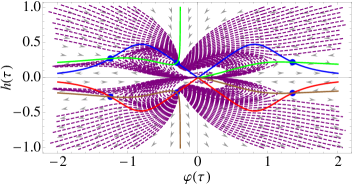
Figure 2: Phase-space diagram in vacuum. The critical points are shown as filled circles, and are found at the intersections of the curves corresponding to $\mbox{d}H/\mbox{d}\tau=0$ and $\mbox{d}\varphi/\mbox{d}\tau=0$ (solid lines). The dashed lines show some particular solutions on this phase space. The arrows depict the arrow of time.

The most important feature of this phase diagram, for us, is that the origin $(\varphi=0,H=0)$ is not a critical point – it corresponds to the crossing of the two branches of the curves $\mbox{d}H/\mbox{d}t=0$. In fact, trajectories coming from below ($H<0$) will necessarily have to go through the origin in a finite interval of time. But the trajectories from below all cross the same point (the origin), which means that (at least for the autonomous system we considered thus far) this point is somehow singular. This means, in our case, that the trajectories passing through the origin will experiment a discontinuous change in the rate of change of $\varphi$ – in other words, one cannot predict the value of $\mbox{d}\varphi/\mbox{d}t$ for trajectories that emerge from the origin at $H=0$.

To see that this is the case, we look for solutions near the origin $\left(\varphi=0,H=0\right)$ of the phase plane. In this limit, the dynamical system can be approximated by

$$\frac{\mbox{d}h}{\mbox{d}\varphi}=h-\frac{\varphi^{2}}{h}+\mathcal{O}\left(h^{2},\varphi^{2},h\varphi\right).$$ (29)

We can rewrite the above equation in terms of $h^{2}$, and then find a first integral of the resulting differential equation. The final result is that

$$h\left(\varphi\right)\simeq\pm\frac{1}{4}\sqrt{A\mbox{e}^{4\varphi}+1+4\varphi\left(1+2\varphi\right)},$$ (30)

where $A$ is an arbitrary integration constant. This means that the 2 dimensional dynamical system is still Lipschitz continuous at the origin (see, e.g., Ref. Jeffreys and Jeffreys (1988), pg. 53), which indicates that the 2 dimensional trajectories can be seen as projections of trajectories in a higher-dimension dynamical phase space. Hence, Eq. (30) indicates that although the two branches ($H>0$ and $H<0$) cannot be simply connected to each other in the case of the 2 dimensional phase space, any enlargement of that phase space will lift the problematic degeneracies.

The saddle points divide the phase diagram in different regions through their separatrices (not shown in Fig. 2, although they can be inferred from the particular solutions.) In particular, the separatrices in the third and fourth quadrants explain why there are solutions which never reach the $H=0$ axis. This is a general feature, in the sense that it does not depend on the matter content: indeed, it follows directly from Eq. (11), which is independent of the matter content for the constrained theory we are considering. However, the evolution of the right-hand side of Eq. (11) being coupled to the matter content through Eq. (15), one expects a similar general behavior in the Hubble parameter for universes with any type of matter content, but with only minor differences in the details of the phase diagram.

Hence, we conclude that a bounce in this constrained gravity theory does seem quite generic, but unfortunately the contracting and expanding branches cannot be connected in a continuous (unambiguous) way to each other, because the dynamical system is two-dimensional. However, as we will show next, the introduction of even a minuscule amount spatial curvature ${\cal K}$, or of any kind of matter, both opening up the phase space into a third dimension, is enough to regularize this bounce, so that every physical variable in the system remains finite and no singularity occurs.

III.2 Spatial curvature

By inspection of the phase diagram of Fig. 2, we can see that for every trajectory in the lower plane ($h<0$) there is a similar trajectory in the upper plane. The only problem is that apparently all these particular solutions cross at the origin $(\varphi=0,h=0)$, which, sadly for the 2 dimensional dynamical system we considered in the previous Section, cannot make sense. As it turns out, spatial curvature is one way to alleviate this problem.

Indeed, with even a small amount of spatial curvature, trajectories coming up from the lower-right corner ($\varphi>0$, $\mbox{d}\varphi/\mbox{d}\tau<0$ $h<0$, $\mbox{d}h/\mbox{d}\tau\gtrsim 0$) emerge from the origin on the upper left corner ($\varphi<0$, $\mbox{d}\varphi/\mbox{d}\tau<0$ $h>0$, $\mbox{d}h/\mbox{d}\tau\gtrsim 0$), and solutions coming up from the lower-left corner emerge on the upper-right corner, so that the particular solutions to the equations of motion are indeed perfectly continuous. This can only happen because the presence of spatial curvature turns our original (flat) 2 dimensional phase space into a 3 dimensional phase space, where $h$ and $a$ are effectively independent dynamical variables. This means that the trajectories of Fig. 2 which cross $\varphi=0$ and $h=0$ can now do so freely, as the third dimension (the scale factor $a$, shown on Fig. 3) opens the possibility that the paths do not cross – in other words, in the 3 dimensional phase space these trajectories actually do not intersect.

To see this, consider the dynamical system composed of Eqs. (19) to (21). The problematic equation, which leads to the difficulties exposed in the previous section, is Eq. (20). In fact, by taking the limit ${\cal H}\rightarrow 0$ at the putative bounce we can see that this equation reduces to

$$\varphi^{\prime}\simeq\frac{1}{2{\cal H}}\left(\frac{a^{2}V}{6}-{\cal K}\right).$$

The rate of change of the scale factor is naturally zero at the bounce (${\cal H}\rightarrow 0$), hence, if the derivative of the field above is finite, then $\varphi\rightarrow\varphi_{\mathrm{B}}$ and $a\rightarrow a_{\mathrm{B}}$ at the bounce. This means that $V(\varphi_{\mathrm{B}})=6{\cal K}/a_{\mathrm{B}}^{2}$, which then implies, for the potential given in Eq. (10), that

$$\varphi_{\mathrm{B}}^{6}=\left(\frac{\Lambda^{2}a_{\mathrm{B}}^{4}}{9{\cal K}^{2}}-1\right)^{-1}.$$ (31)

Clearly, as ${\cal K}\rightarrow 0^{\pm}$, $\varphi_{\mathrm{B}}\rightarrow 0$, which means that the physical system itself is perfectly well-behaved for any nonzero value of ${\cal K}$.

Hence, we conclude that it is possible to connect the two branches of the theory (the contracting and expanding phases), provided that there is any amount of curvature, however small. Since the limit ${\cal K}\rightarrow 0$ is well-behaved, we can do without it entirely, and join the pieces of the trajectories between the two branches, constructing zero-curvature bounce models.

Figure 3: Scale factor $a(\tau)$ (left panel), reduced Hubble parameter $h(\tau)$ (center) and scalar field $\varphi(\tau)$ (right panel) as a function of time for almost vanishing curvature (${\cal K}=10^{-9}$, full line) and small but non vanishing curvature (${\cal K}=10^{-3}$ and ${\cal K}=10^{-2}$, respectively dashed and dotted lines). It is interesting to note that the vanishing curvature limit allows for a so-called emerging Universe model in which the scale factor is essentially constant for a long period of time after which expansion (in fact inflation) takes place spontaneously. Pushing the calculation backwards in time shows that the vanishing of the Hubble rate is only stable in the actual limit ${\cal K}\to 0$: expansion begins after a finite amount of time, but the amount of past-time during which $h=0$ can only be made infinite provided ${\cal K}=0$ strictly; otherwise, the Minkowski state always originates from a contracting de Sitter phase.

It is also interesting to notice that the condition (31) implies that there is a maximum value for the spatial curvature

$$\left|{\cal K}_{\mathrm{max}}\right|=\frac{\Lambda a_{\mathrm{B}}^{2}}{3}=H_{\Lambda}^{2}a_{\mathrm{B}}^{2},$$ (32)

which is in fact perfectly legitimate in our constrained theory, since we limit the spacetime curvature at all times – and that includes the time of the bounce itself. These considerations are illustrated on Fig. 3, showing the time evolution of the scale factor, the reduced Hubble rate and the scalar field, for three scenarios with different values of the spatial curvature.

III.3 Constrained gravity with a matter fluid

Having established that, qualitatively, spatial curvature does nothing to our model, let us continue with the analysis of the field equations in the flat case, but now in the presence of matter. We will show in what follows that since the introduction of matter enlarges the dimensionality of the phase space, it similarly allows the trajectories in the contracting and expanding branches to be joined – whatever the amount of matter present.

If $\rho$ is the matter energy density, then the system will acquire one more degree of freedom, that is, our dynamical equations are Eqs. (24), (25) and (26), which take the form

$$\frac{\mbox{d}h}{\mbox{d}\tau} = -h^{2}+\frac{\varphi^{2}}{2\left(1+\varphi^{6}\right)^{3/2}},$$ (33)

$$\frac{\mbox{d}\varphi}{\mbox{d}\tau} = -\frac{1}{2}h\left(1+4\varphi\right)+\frac{\varphi^{3}}{6h\sqrt{1+\varphi^{6}}}+\frac{\varepsilon}{2h},$$ (34)

$$\frac{\mbox{d}\varepsilon}{\mbox{d}\tau} = -3h\left(1+w\right)\varepsilon,$$ (35)

where, as usual, $w\equiv p/\rho=\mathcal{P}/\varepsilon$ is the equation of state for the fluid ($w=0$ for dust, $w=\frac{1}{3}$ for radiation, and $w=-\frac{1}{3}$ for a curvature-like matter.)

Before proceeding with the detailed analysis of the phase space of this dynamical system, let us concentrate on a particular class of solutions of the system (33)-(35) which gives us some information on how matter affects the bounce. For this purpose, let us return to the previous vacuum case, Eqs. (27) and (28). We have seen that, in our model, not only $h\rightarrow 0$ at the bounce, but also that $\mbox{d}h/\mbox{d}\tau$ and $\mbox{d}\varphi/\mbox{d}\tau$ vanish there. The evolution at the bounce is therefore dominated by the higher time derivatives – which can be tuned, through the initial conditions, to small values, making the duration of the bounce very large. This means that, depending on the initial conditions of the Universe, the spacetime can stay in this quasi-Minkowski ($h=0$) state for a long period of cosmic time before undergoing a phase of acceleration with $\mbox{d}h/\mbox{d}\tau>0$. However, we see that in the presence of matter the Universe starts in a de Sitter contracting phase and quickly evolves towards the bounce, emerging in a super-inflationary period before reaching the ever-expanding de Sitter phase. This is exactly similar to what we found for the curvature case and exemplified in Fig. 4.

Figure 4: Time evolution of the Hubble rate in vacuum (full line) and with matter (dashed). When a small quantity of radiation is added to the system [$\rho_{\mathrm{rad}}\left(0\right)=10^{-5}$ in this example], the scale factor evolves from a contracting de Sitter phase to the bounce. The final state corresponds to an ever-expanding de Sitter period. The results are exactly similar when, instead of radiation, one considers dust or a curvature-like fluid. The three cases are shown in Fig. 5. It is worth noticing that the presence of the fluid dramatically reduces the bounce duration so that an emergent universe model in this case is very unlikely.

Figure 5: Time evolution of the densities when the fluid consists of dust ($w=0$, full line), radiation ($w=\frac{1}{3}$, dashed line) and curvature ($w=-\frac{1}{3}$, dotted line) Hubble rate in vacuum (full line) and with matter (dashed).

Figure 6: Effect of including matter on the scalar field as a function of time. The full line represents the scalar field evolution in vacuum, while the dashed line includes a dust or radiation component (both curves are indistinguishable).

Notice that, as mentioned before, with matter we do not have a phase plane anymore – the phase space has three dimensions. The possible trajectories that can be achieved in the projected phase space $(\varphi,h)$ are essentially the same as those obtained in the 2 dimensional case of Fig. (2).

Thus we have been able to set up the cosmology for a homogeneous, spatially flat and isotropic universe filled uniquely with dust and radiation and that behaves as follows: the universe starts contracting until it reaches a minimum radius, when it bounces and expands afterwards. The expansion period right after the bounce corresponds to a super-inflationary period ($\mbox{d}h/\mbox{d}\tau>0$). When the Hubble parameter reaches a certain maximum value (which depends on the details of the spacetime constraints), it starts to decrease, similarly as in the usual FLRW universe, until it reaches either a de Sitter attractor or some other regime as its final state.

The behaviors discussed above are generic and do not depend crucially on the choice (10) for the potential. To see this, we considered many different potentials, and, as a matter of example, we show on Fig. 7 the phase diagram obtained for the choice

$$V_{2}\left(\varphi\right)=\frac{2\Lambda\varphi}{\sqrt{1+\varphi^{6}}},$$ (36)

which is represented on Fig. 8.

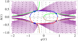
Figure 7: Phase diagram for the potential $V_{2}$ given by Eq. (36) displayed on Fig. 8.

Figure 8: The potential $V_{2}(\varphi)$ (full line) and its derivative (dashed) used to derive the phase portrait of Fig. 7.

III.4 Bounce Scale

In this subsection our aim is to calculate the characteristic time scale of the bounce described by the above model. More specifically, we will show that, in contrast to the general relativistic description Abramo and Peter (2007); Martin and Peter (2003), the typical bounce time scale can be made arbitrarily small in this category of theories.

Let us start with the following expansion Martin and Peter (2003) for the scale factor around the bounce

$$a\left(\eta\right)=a_{0}\left[1+\frac{1}{2}\left(\frac{\eta}{\eta_{0}}\right)^{2}+\delta\left(\frac{\eta}{\eta_{0}}\right)^{3}+\frac{5}{24}\left(1+\xi\right)\left(\frac{\eta}{\eta_{0}}\right)^{4}\right],$$ (37)

where we have set the bounce time as the origin of conformal time, i.e., $\eta_{\mathrm{bounce}}=0$. In Eq. (37), $\eta_{0}$ provides the bounce characteristic time scale. Similarly, any other quantity with $0$ as a subscript means that this quantity is to be evaluated when the bounce occurs, i.e. for $\eta=0$. As explained in Ref. Martin and Peter (2003), the parameters $\delta$ and $\xi$ control the amplitude of the deviation from the de Sitter-like bounce, whose scale factor is given by $a\left(\eta\right)=a_{0}\sqrt{1+\tan^{2}\left(\eta/\eta_{0}\right)}$, thereby explaining the factor $5/24$ in front of the fourth term in Eq.  (37).

In a similar way as for the scale factor, we assume that the scalar field $\varphi\left(\eta\right)$, its potential $V\left(\eta\right)$ and the energy density $\rho\left(\eta\right)$ all have a Taylor expansion about $\eta=0$, that is we set

$$\varphi\left(\eta\right) = \varphi_{0}+\varphi_{1}\left(\frac{\eta}{\eta_{0}}\right)+\varphi_{2}\left(\frac{\eta}{\eta_{0}}\right)^{2}+\varphi_{3}\left(\frac{\eta}{\eta_{0}}\right)^{3}+\cdots$$ (38)

$$V\left(\eta\right) = V_{0}+V_{1}\left(\frac{\eta}{\eta_{0}}\right)+V_{2}\left(\frac{\eta}{\eta_{0}}\right)^{2}+V_{3}\left(\frac{\eta}{\eta_{0}}\right)^{3}+\cdots$$ (39)

$$\rho\left(\eta\right) = \rho_{0}+\rho_{1}\left(\frac{\eta}{\eta_{0}}\right)+\rho_{2}\left(\frac{\eta}{\eta_{0}}\right)^{2}+\rho_{3}\left(\frac{\eta}{\eta_{0}}\right)^{3}+\cdots,$$ (40)

where the parameters $\varphi_{i}$, $V_{i}$ and $\rho_{i}$ are to be determined below.

In order to determine the defining parameters of the scale factor, and hence the bounce scale itself, it is sufficient to verify in what manner they are constrained by the field equations. In practice, we insert the expansion (37) into Eqs. (19), (20) and (21) and identify terms order by order in $\eta/\eta_{0}\ll 1$. This leads to

$$\rho_{1} = 0,$$ (41)

$$\rho_{2} = -\frac{3}{2}(1+w)\rho_{0},$$ (42)

$$\rho_{3} = -3\delta(1+w)\rho_{0},$$ (43)

which expresses the first terms in the energy density. Note at this point that a symmetric bounce, having $\delta=0$, leads to an even behavior for the density, as expected. The first equality merely expresses energy conservation at the bounce conformal time.

The cosmic time bounce duration $t_{0}$ can then be evaluated as

$$t_{0}^{2}\equiv a_{0}^{2}\eta_{0}^{2}=\frac{12\varphi_{1}}{V_{1}}=12\left(\left.\frac{\mbox{d}V}{\mbox{d}\varphi}\right|_{0}\right)^{-1},$$ (44)

where the last term is the derivative of the potential with respect to $\varphi$ evaluated at the bounce conformal time $\eta=0$; this remains a free parameter, as can be seen from inspection of the following relations

$$V_{0} = \frac{6{\cal K}}{a_{0}^{2}}-16\pi G_{{}_{\mathrm{N}}}\rho_{0},$$ (45)

$$V_{2} = \left.\frac{\mbox{d}V}{\mbox{d}\varphi}\right|_{0}\left(3\delta\varphi_{1}+\varphi_{2}\right),$$ (46)

relating the parameters for the scalar field potential. Note at this point that for negative or vanishing curvature ${\cal K}$, the potential needs to be negative at the bounce, so that, as in GR, a simple massive scalar field cannot lead to a bouncing phase unless the Universe is closed.

At the next orders, we obtain relationship between the higher derivatives of the scalar field at the bounce and the energy density at that point as well as the asymmetry of the bounce, namely

$$\varphi_{2} = -\frac{1}{2}\left(1+4\varphi_{0}\right)+6\left(\left.\frac{\mbox{d}V}{\mbox{d}\varphi}\right|_{0}\right)^{-1}\left[\frac{{\cal K}}{a_{0}^{2}}-4\pi G_{{}_{\mathrm{N}}}\rho_{0}\left(1+w\right)\right],$$ (47)

$$\varphi_{3} = -\delta\left(1+4\varphi_{0}\right)-\frac{2}{3}\varphi_{1},$$ (49)

and finally one can identify the fourth order term in the scale factor expansion $\xi$ as

$$\xi = \frac{6}{5}\left\{\frac{1}{V_{1}}\left[V_{3}+24\pi G_{{}_{\mathrm{N}}}\delta\rho_{0}\left(1+w\right)-24\delta\frac{{\cal K}}{a_{0}^{2}}\right]\right.$$ (51)

$$\hskip 56.9055pt+\left.\frac{2\delta\left(1+4\varphi_{0}\right)-\varphi_{3}}{\varphi_{1}}\right\}.$$

An important conclusion that can be drawn from these simple relations is that the bounce scale can be made as small as one wants. Clearly, we see that the larger the derivative of the potential at the bounce or, put in another way, the larger the constant $\sqrt{\Lambda}$ which defines the dimension of $V\left(\varphi\right)$ is, the smaller the bounce characteristic conformal time scale will be, for a given bounce length scale $a_{0}$. This result can be consistently checked by numerical integration of system (20): consider the vacuum equations of the last subsection, Eqs. (27) and (28). At the point $\left(\varphi=0,h=0\right)$, we recall that the derivative of the potential is exactly zero. But, according to the relation (44), this implies that the physical time duration $t_{0}=a_{0}\eta_{0}$ of the bounce goes to infinity or, put in another way, that there is no bounce at all. This confirms the results for vacuum obtained in the last section.

IV Conclusion

Cosmological inflation now probably deserves to be included in the standard picture of the Universe. However, as inflation cannot be directly observed, it is desirable to find other, challenging models that could similarly solve the problems of non inflationary cosmology while at the same time making different predictions for data sets – some of which may yet be observed as, e.g., non gaussianity or tensor modes of perturbations. Such a non-inflationary model could include a phase of contraction followed by a bounce, leading to the current expansion.

Having a bouncing phase in the early Universe is a highly non-trivial demand in the framework of general relativity with well-behaved matter content. It usually requires a strictly positive value for the spatial curvature, in contradiction with the current observational data. Therefore, unless a phase of inflation is invoked after the bounce occurred, either the matter content or the gravity theory must be changed.

The simplest way for a bounce to take place in a regular matter theory consists in demanding a positive spatial curvature to compensate for the positive energy density of matter, allowing the Hubble parameter to vanish at the bounce. But by doing so, it was found that the time duration of the bounce was bounded from below so that an arbitrary short bounce could not take place. It was suggested that this was entirely due to the curvature, whose value was indeed crucial in limiting the bounce duration.

In this paper our main purpose was to investigate a non singular bounce in the framework of the modified gravity model of Brandenberger et al. (1993). We found solutions for which the universe is described by a period of contraction followed by an expanding, super-inflationary phase before connecting to a more usual radiation- or matter-dominated epoch of the FLRW universe. The final period then emerges as an ever-expanding de Sitter universe. We have computed the duration of the bounce for that model, and we found that, whatever the bounce, irrespectively of whether or not it is symmetric, whether or not there is spatial curvature (independently of the sign of this curvature), and whether in vacuum or not, its typical duration is unconstrained.

This arbitrariness in the duration of the bounce could have important consequences for the evolution of fluctuations through the bounce. However, although the background models are ruled by second-order equations, perturbations will almost surely show signs of the underlying instability of our higher-order gravity model, so at this stage it is not clear that perturbations in the framework of our models could be sensible.

Acknowledgements

R. A. and I. Y. would like to thank the Institut d’Astrophysique de Paris, and P. P., the Instituto de Física da Universidade de São Paulo, for their warm hospitality. We also would like to thank FAPESP, CNPq and CAPES of Brazil, and COFECUB of France, for financial support.

References

- Komatsu et al (2009) E. Komatsu et al, Ap. J. Supp. 180, 330 (2009), eprint 0803.0547.
- Guth (1981) A. H. Guth, Phys. Rev. D 23, 347 (1981).
- Linde (1982) A. D. Linde, Phys. Lett. B108, 389 (1982).
- Albrecht and Steinhardt (1982) A. Albrecht and P. J. Steinhardt, Phys. Rev. Lett. 48, 1220 (1982).
- Borde and Vilenkin (1997) A. Borde and A. Vilenkin, Phys. Rev. D 56, 717 (1997).
- Borde and Vilenkin (1994) A. Borde and A. Vilenkin, Phys. Rev. Lett. 72, 3305 (1994).
- Borde et al. (2003) A. Borde, A. H. Guth, and A. Vilenkin, Phys. Rev. Lett. 90, 151301 (2003).
- Gasperini et al. (2003) M. Gasperini, M. Giovannini, and G. Veneziano, Phys. Rep. 373, 1 (2003).
- Lidsey et al. (2000) J. E. Lidsey, D. Wands, and E. J. Copeland, Physics Reports 337, 343 (2000).
- Murphy (1973) G. L. Murphy, Phys. Rev. D 8, 4231 (1973).
- Melnikov and Orlov (1979) V. N. Melnikov and S. V. Orlov, Phys. Lett. A 70, 263 (1979).
- Fabris et al. (2003) J. C. Fabris, R. G. Furtado, P. Peter, and N. Pinto-Neto, Phys. Rev. D 67, 124003 (2003).
- Martin and Peter (2003) J. Martin and P. Peter, Phys. Rev. D68, 103517 (2003), eprint hep-th/0307077.
- Martin et al. (2002) J. Martin, P. Peter, N. Pinto Neto, and D. J. Schwarz, Phys. Rev. D65, 123513 (2002), eprint hep-th/0112128.
- Veneziano (1997) G. Veneziano (1997), eprint hep-th/9802057.
- Brustein and Veneziano (1994) R. Brustein and G. Veneziano, Phys. Lett. B329, 429 (1994), eprint hep-th/9403060.
- Finelli and Brandenberger (1999) F. Finelli and R. Brandenberger, Phys. Rev. Lett. 82, 1362 (1999).
- Mukhanov et al. (1992) V. F. Mukhanov, H. A. Feldman, and R. H. Brandenberger, Phys. Rept. 215, 203 (1992).
- Durrer and Vernizzi (2002) R. Durrer and F. Vernizzi, Phys. Rev. D 66, 083503 (2002).
- Martin and Peter (2004) J. Martin and P. Peter, Phys. Rev. Lett. 92, 061301 (2004).
- Armendariz-Picon et al. (2001) C. Armendariz-Picon, V. F. Mukhanov, and P. J. Steinhardt, Phys. Rev. D63, 103510 (2001), eprint astro-ph/0006373.
- Abramo and Peter (2007) L. R. Abramo and P. Peter, JCAP 0709, 001 (2007), eprint arXiv:0705.2893 [astro-ph].
- Mukhanov and Brandenberger (1992) V. F. Mukhanov and R. H. Brandenberger, Phys. Rev. Lett. 68, 1969 (1992).
- Brandenberger et al. (1993) R. Brandenberger, V. Mukhanov, and A. Sornborger, Phys. Rev. D 48, 1629 (1993).
- Brandenberger et al. (1998) R. H. Brandenberger, R. Easther, and J. Maia, JHEP 08, 007 (1998), eprint gr-qc/9806111.
- ’t Hooft and Veltman (1974) G. ’t Hooft and M. J. G. Veltman, Annales Inst. H. Poincar A20, 69 (1974).
- Deser et al. (1974) S. Deser, H.-S. Tsao, and P. van Nieuwenhuizen, Phys. Rev. D 10, 3337 (1974).
- Stelle (1977) K. S. Stelle, Phys. Rev. D 16, 953 (1977).
- Chiba (2005) T. Chiba, JCAP 0503, 008 (2005), eprint gr-qc/0502070.
- Nunez and Solganik (2005) A. Nunez and S. Solganik, Phys. Lett. B608, 189 (2005), eprint hep-th/0411102.
- Woodard (2007) R. P. Woodard, Lect. Notes Phys. 720, 403 (2007), eprint astro-ph/0601672.
- Bruneton and Esposito-Farese (2007) J.-P. Bruneton and G. Esposito-Farese, Phys. Rev. D76, 124012 (2007), eprint 0705.4043.
- Jeffreys and Jeffreys (1988) H. Jeffreys and B. S. Jeffreys, Methods of Mathematical Physics, 3rd Ed. (Cambridge, UK: Cambridge University Press, 1988).