Polarization Changes of Pulsars due to Wave Propagation Through Magnetospheres

Abstract

We study the propagation effects of radio waves in a pulsar magnetosphere, composed of relativistic electron-positron pair plasmas streaming along the magnetic field lines and corotating with the pulsar. We critically examine the various physical effects that can potentially influence the observed wave intensity and polarization, including resonant cyclotron absorption, wave mode coupling due to pulsar rotation, wave propagation through quasi-tangential regions (where the photon ray is nearly parallel to the magnetic field) and mode circularization due to the difference in the electron/positron density/velocity distributions. We numerically integrate the transfer equations for wave polarization in the rotating magnetosphere, taking account of all the propagation effects in a self-consistent manner. For typical magnetospheric plasma parameters produced by pair cascade, we find that the observed radio intensity and polarization profiles can be strongly modified by the propagation effects. For relatively large impact parameter (the minimum angle between the magnetic dipole axis and the line of sight), the polarization angle profile is similar to the prediction from the Rotating Vector Model, except for a phase shift and an appreciable circular polarization. For smaller impact parameter, the linear polarization position angle may exhibit a sudden $90^{o}$ jump due to the quasi-tangential propagation effect, accompanied by complex circular polarization profile. Some applications of our results are discussed, including the origin of non-gaussion pulse profiles, the relationship between the position angle profile and circular polarization in conal-double pulsars, and the orthogonal polarization modes.

1 Introduction

Pulsar radio emission is likely generated within a few hundred kilometers from the neutron star (NS) surface (e.g. Cordes 1978; Blaskiewicz et al. 1991; Kramer et al. 1997; Kijak & Gil 2003). A pulsar is surrounded by a magnetosphere filled with relativistic electron-positron pair plasmas (plus possibly a small amount of ions) within the light cylinder. When radio waves propagate though the magnetosphere, the total flux, polarization state and spectrum of the emission may be modified by propagation effects. Understanding the property of wave propagation in pulsar magnetospheres is necessary for the interpretation of various observations of pulsars.

Radio emission from pulsars shows strong linear polarization. For some pulse components or even the whole pulse profiles it can be 100% percent polarized (e.g. Lyne & Manchester 1988; Gould & Lyne 1998; Weisberg et al. 1999, 2004; Han et al. 2009). Linear polarization (LP) is closely related to magnetic field lines where the emission was generated. Based on the linear polarization position angle (PA) curve of Vela pulsar, the Rotating-Vector-Model (RVM) was suggested by Radhakrishnan & Cooke (1969). For some pulsars, especially the so-called conal-double type pulsars, RVM works very well (e.g., Mitra & Li 2004). However, the PA curves of most pulsars are much more complex and do not follow the simple RVM model. The deviation from the RVM model could be caused by the intrinsic emission mechanism (e.g., Blaskiewicz et al. 1991), which is highly uncertain (e.g., Lyubarsky 2008), and/or the propagation effect through the pulsar magnetosphere (see below). Also, the PA curves or polarization observations of individual pulses show the orthogonal polarization modes (OPM) phenomenon, in which the polarization position angle exhibits a sudden $\sim 90^{\circ}$ jumps (e.g. Manchester et al. 1975; Backer et al. 1976; Cordes et al. 1978; Stinebring et al. 1984a, 1984b; Xilouris et al. 1995). It is not clear whether the OPM arises from the emission process (e.g. Luo & Melrose 2004) or the propagation effect (e.g. McKinnon & Stinebring 2000).

Another important observational feature of pulsar radio emission is the circular polarization (CP, e.g. Rankin 1983; Radhakrishnan & Rankin 1990; Han et al. 1998). Significant CPs have been observed in individual pulses of pulsars with mean values typically 20%–30%. Very high degrees of CP are occasionally observed from some components of pulsar profiles (e.g. Cognard et al. 1996; Han et al. 2009). Radhakrishnan & Rankin (1990) identified two main types of CP signature: antisymmetric type with sign reverse in the mid-pulse and symmetric type without sign change over whole profile. They concluded that the CP of the antisymmetric type is associated with the core emission and strongly correlated with the sense of rotation of the linear position angle. Han et al. (1998) showed that this correlation is not kept for a larger sample, and they found that for conal-double pulsars the sense of CP is correlated with the sense of PA curves.

The diverse behaviours of pulsar polarization (including LP and CP) may require more than one mechanisms for proper explanations. First, they may be caused by an intrinsic mechanism in the emission region and/or process. For example, Randhakrishnan & Rankin (1990) suggested that geometrical effect to the pulsar beam from curvature radiation can naturally generate antisymmetric circular polarization for the core components. Gangadhara (1997) suggested that the observed circular polarization could be caused by the coherent superposition of two orthogonal modes emitted by positrons and electrons. Xu et al. (2000) interpreted the circular polarization by the superposition of coherent inverse Compton scattering. Kazbegi et al. (1991) suggested that cyclotron instability may be responsible for the circular polarization. Also, Luo & Melrose (2001) suggested that circular polarization can develop by cyclotron absorption when the distributions (especially the number densities) of the magnetospheric electrons and positrons are different.

However, many observed characteristics of the pulsar radio emision are most likely dictated by the wave propagation in the magnetospheric plasma (see, e.g., Melrose 2003 and Lyubarsky 2008 for a review). A number of theoretical works have been devoted to study how magnetosphere propagation influences pulsar polarization observations. Whatever the emission mechanism, radio wave propagates in the plasma in the form of two orthogonally polarized normal modes. The polarization state of the wave evolves along the ray, following the direction of the local magnetic field, a process termed “adiabatic walking” (Cheng & Ruderman 1979). Cheng & Ruderman (1979) introduced two propagation effects: the wave mode coupling effect for pure pair plasma and the circularization effect (natural modes become circular polarized), both of which can generate circular polarization. Melrose (1979) and Allen & Melrose (1982) suggested that the separation of natural waves (because of different refractive indices) can cause the OPM phenomenon. Arons & Barnard (1986) studied the wave dispersion relation and natural modes in the relativistic pair plasma. Lyubaskii & Petrova (1999) considered the natural modes in relativistic plasma with co-rotating velocity in the infinite magnetic field limit, and Petrova & Lyubarskii (2000) studied refraction and polarzation transfer in such a plasma. Luo & Melrose (2001) and Fussell et al. (2003) studied the cyclotron absorption of radio emission within pulsar magnetospheres. Petrova (2006) further studied the polarization transfer in pulsar magnetosphere and considered the wave mode coupling and cyclotron absorption effect. Johnston et al. (2005) suggested that the variation of circular polarization of PSR B1259$-$63 during the elipse with its main-sequence companion is related to the wave propagation effect in the magnetosphere of the companion star. However, none of the previous studies have calculated the final polarization profiles with all of these propagation effects included in a self-consistent way within a single theoretical framework. It is often unclear which of the effects are most important, and if so, under what conditions. In this paper we attempt to combine all the propagation effects, evaluate their relative importance, and use numerical integration along the photon ray to study the influence of propagation effects on the final polarization states.

This paper is organized as follows. In section 2, we present the geometrical model for our calculation and the general wave evolution equation in a magnetized plasma. In section 3, we give the expression of the dielectric tensor of a relativistic pair plasma characterizing the magnetosphere of a pulsar, and discuss the natural wave modes and their evolution. In section 4, we study several important propagation effects separately: cyclotron absorption, wave mode coupling, circularization and the quasi-tangential propagation (see Wang & Lai 2009). In section 5, we present numerical calculations of the single photon evolution and the phase profiles of pulsar emission beam. Our results and possible applications are presented in section 6.

2 Geometry and General Wave Evolution Equation

2.1 Geometrical Model

Consider a photon (radio wave) emitted at the initial position $\mn@boldsymbol{r}_{\rm i}$ at time $t_{\rm i}$ (corresponding to the pulsar rotation phase $\Psi_{\rm i}$). Suppose the photon trajectory is a straight line along ${\mn@boldsymbol{k}}$ (the wave vector). In a fixed $XYZ$ frame with $\hat{\mn@boldsymbol{Z}}=\hat{\mn@boldsymbol{k}}$ along the line of sight and $\mn@boldsymbol{\Omega}$ (the pulsar spin vector) in the $XZ$-plane ($\hat{\mn@boldsymbol{Z}}\times\hat{\mn@boldsymbol{\Omega}}=\sin\zeta\hat{\mn@boldsymbol{Y}}$, here $\zeta$ is the angle between ${\mn@boldsymbol{k}}$ and $\mn@boldsymbol{\Omega}$; see Fig. 1), the photon position after emission and the corresponding pulsar rotation phase are

$$\mn@boldsymbol{r}=\mn@boldsymbol{r}_{\rm i}+s\hat{\mn@boldsymbol{Z}},$$ (2.1)

$$\Psi=\Psi_{\rm i}+\Omega(t-t_{i})=\Psi_{\rm i}+s/r_{\rm lc},$$ (2.2)

where $s=c(t-t_{\rm i})$ is the distance from the emission point along the ray, and $r_{\rm lc}=c/\Omega$ the radius of the light cylinder. The rotating magnetic field is given by

$$\mn@boldsymbol{B}(s)=-\nabla(\mn@boldsymbol{\mu}\cdot\mn@boldsymbol{r}/r^{3})=-\frac{\mn@boldsymbol{\mu}}{r^{3}}+\frac{3\mn@boldsymbol{r}}{r^{5}}(\mn@boldsymbol{\mu}\cdot\mn@boldsymbol{r}),$$ (2.3)

with

$$\mn@boldsymbol{\mu}(s)=\mu\left[(\sin\zeta\cos\alpha-\cos\zeta\sin\alpha\cos\Psi)\hat{\mn@boldsymbol{X}}-\sin\alpha\sin\Psi\hat{\mn@boldsymbol{Y}}+(\cos\zeta\cos\alpha+\sin\zeta\sin\alpha\cos\Psi)\hat{\mn@boldsymbol{Z}}\right],$$ (2.4)

where $\alpha$ is the inclination angle between $\mn@boldsymbol{\Omega}$ and $\mn@boldsymbol{\mu}$ (see Fig. 1). Note that the impact angle $\chi$, which is the smallest angle between ${\mn@boldsymbol{k}}$ and $\mn@boldsymbol{\mu}$, is given by $\chi=\zeta-\alpha$. Thus, the polar angles of $\mn@boldsymbol{\mu}$ in $XYZ$ frame, ($\theta_{\mu}$, $\phi_{\mu}$), are given by

$$\cos\theta_{\mu}=\cos\zeta\cos\alpha+\sin\zeta\sin\alpha\cos\Psi,\\ \tan\phi_{\mu}=\frac{-\sin\alpha\sin\Psi}{\sin\zeta\cos\alpha-\cos\zeta\sin\alpha\cos\Psi}.$$ (2.5)

The magnetic field at a given point along the ray is inclined at an angle $\theta_{B}$ with respect to the line of sight, and make an azimuthal angle $\phi_{B}$ in the $XY$-plane such that:

$$\cos\theta_{B}(s)=\frac{B_{Z}}{B},\quad\tan\phi_{B}(s)=\frac{B_{Y}}{B_{X}}.$$ (2.6)

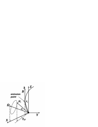
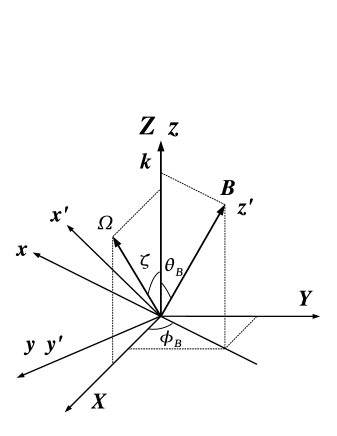
Figure 1: Three frames used in this paper: 1) The fixed frame $XYZ$ with $\hat{\mn@boldsymbol{Z}}\parallel\hat{\mn@boldsymbol{k}}$, $\mn@boldsymbol{\Omega}$ in the $XZ$-plane and $\hat{\mn@boldsymbol{k}}\times\hat{\mn@boldsymbol{\Omega}}=\Omega\sin\zeta\hat{\mn@boldsymbol{Y}}$. The direction of $\mn@boldsymbol{B}$ in this frame is ($\theta_{B},\phi_{B}$); 2) The instantaneous inertial frame $xyz$ with $\hat{\mn@boldsymbol{z}}=\hat{\mn@boldsymbol{Z}}$, $\mn@boldsymbol{B}$ in the $xz$-plane and $\hat{\mn@boldsymbol{k}}\times\hat{\mn@boldsymbol{B}}=-\sin\theta_{B}\hat{\mn@boldsymbol{y}}$; 3) The instantaneous inertial frame $x^{\prime}y^{\prime}z^{\prime}$ with $\hat{\mn@boldsymbol{z}}^{\prime}=\hat{\mn@boldsymbol{B}}$, ${\mn@boldsymbol{k}}$ in the $x^{\prime}z^{\prime}$-plane and $\hat{\mn@boldsymbol{k}}\times\hat{\mn@boldsymbol{B}}=-\sin\theta_{B}\hat{\mn@boldsymbol{y}}^{\prime}$.

2.2 Wave Evolution Equations

The wave equation for photon propagation takes the form

$$\nabla\times({{\mn@boldsymbol{\mu}}^{-1}}\cdot\nabla\times{\mn@boldsymbol{E}})={\omega^{2}\over c^{2}}{\mn@boldsymbol{\mn@boldsymbol{\epsilon}}}\cdot\mn@boldsymbol{E},$$ (2.7)

where $\mn@boldsymbol{E}$ is the electric field, and $\mn@boldsymbol{\mn@boldsymbol{\epsilon}}$, $\mn@boldsymbol{\mu}^{-1}$ are the dielectric and inverse permeability tensors, respectively. The inverse permeability is very close to unity when $B\ll B_{\rm Q}=4.414\times 10^{13}$ G (the critical QED field strength), and we set ${\mn@boldsymbol{\mu}}$ to be unity in the remainder of the paper. In practice, it is most convenient to calculate dielectric tensor in the $x^{\prime}y^{\prime}z^{\prime}$ frame (where the $z^{\prime}$-axis is along $\mn@boldsymbol{B}$, and ${\mn@boldsymbol{k}}$ in the $x^{\prime}z^{\prime}$-plane, see Fig. 1). Once ${\mn@boldsymbol{[\mn@boldsymbol{\epsilon}]}}_{x^{\prime}y^{\prime}z^{\prime}}$ (the matrix representation of the dielectric tensor in the $x^{\prime}y^{\prime}z^{\prime}$ frame) is known, we can easily obtain ${\mn@boldsymbol{[\mn@boldsymbol{\epsilon}]}}_{XYZ}$ in the fixed $XYZ$ frame through a coordinate transformation

$${\mn@boldsymbol{[\mn@boldsymbol{\epsilon}]}}_{XYZ}=\mn@boldsymbol{M}{\mn@boldsymbol{[\mn@boldsymbol{\epsilon}]}}_{x^{\prime}y^{\prime}z^{\prime}}\mn@boldsymbol{M}^{T},$$ (2.8)

where the transformation matrix $\mn@boldsymbol{M}$ is

$$\mn@boldsymbol{M}=\left(\begin{array}[]{ccc}-\cos\phi_{B}&\sin\phi_{B}&0\\ -\sin\phi_{B}&-\cos\phi_{B}&0\\ 0&0&1\end{array}\right)\left(\begin{array}[]{ccc}\cos\theta_{B}&0&-\sin\theta_{B}\\ 0&1&0\\ \sin\theta_{B}&0&\cos\theta_{B}\end{array}\right)=\left(\begin{array}[]{ccc}-\cos\theta_{B}\cos\phi_{B}&\sin\phi_{B}&\sin\theta_{B}\cos\phi_{B}\\ -\cos\theta_{B}\sin\phi_{B}&-\cos\phi_{B}&\sin\theta_{B}\sin\phi_{B}\\ \sin\theta_{B}&0&\cos\theta_{B}\end{array}\right)$$ (2.9)

and $\mn@boldsymbol{M}^{T}$ is the transpose matrix of $\mn@boldsymbol{M}$.

Knowing $\mn@boldsymbol{\mn@boldsymbol{\epsilon}}$ along the trajectory, we can use eq. (2.7) to derive the wave amplitude evolution equation. Let $\mn@boldsymbol{E}=e^{ik_{0}s}\mn@boldsymbol{A}$, where $k_{0}=\omega/c$. Assuming that $|d\mn@boldsymbol{A}/{\rm d}s|\ll k_{0}|\mn@boldsymbol{A}|$ (geometric optics approximation), we obtain

$$\frac{{\rm d}}{{\rm d}s}\left(\begin{array}[]{c}A_{X}\\ A_{Y}\end{array}\right)={ik_{0}\over 2}\left[\begin{array}[]{cc}\sigma_{XX}&\sigma_{XY}\\ \sigma_{YX}&\sigma_{YY}\end{array}\right]\left(\begin{array}[]{c}A_{X}\\ A_{Y}\end{array}\right),$$ (2.10)

where

$$\sigma_{XX} = \epsilon_{XX}-1,$$

$$\sigma_{XY} = \epsilon_{XY},$$

$$\sigma_{YX} = \epsilon_{YX},$$

$$\sigma_{YY} = \epsilon_{YY}-1.$$ (2.11)

The wave evolution equation (2.10) can be used to study the evolution of EM wave amplitude across the pulsar magnetosphere.

We can also follow the evolution of the four Stokes parameters instead of the evolution of the wave amplitudes. The four Stokes parameters are defined by (in the fixed $XYZ$ frame)

$$I = A_{X}A_{X}^{\ast}+A_{Y}A_{Y}^{\ast},$$

$$Q = A_{X}A_{X}^{\ast}-A_{Y}A_{Y}^{\ast},$$

$$U = A_{X}A_{Y}^{\ast}+A_{Y}A_{X}^{\ast},$$

$$V = -i(A_{X}A_{Y}^{\ast}-A_{Y}A_{X}^{\ast}).$$ (2.12)

Combining with eq. (2.10), we obtain the evolution equations for the Stokes parameters:

$$\frac{{\rm d}I}{{\rm d}s} = -k_{0}\frac{\sigma_{XX,i}+\sigma_{YY,i}}{2}I-k_{0}\frac{\sigma_{XX,i}-\sigma_{YY,i}}{2}Q-k_{0}\frac{\sigma_{XY,i}+\sigma_{YX,i}}{2}U-k_{0}\frac{\sigma_{XY,r}-\sigma_{YX,r}}{2}V,$$

$$\frac{{\rm d}Q}{{\rm d}s} = -k_{0}\frac{\sigma_{XX,i}-\sigma_{YY,i}}{2}I-k_{0}\frac{\sigma_{XX,i}+\sigma_{YY,i}}{2}Q-k_{0}\frac{\sigma_{XY,i}-\sigma_{YX,i}}{2}U+k_{0}\frac{\sigma_{XY,r}+\sigma_{YX,r}}{2}V,$$

$$\frac{{\rm d}U}{{\rm d}s} = -k_{0}\frac{\sigma_{XY,i}+\sigma_{YX,i}}{2}I+k_{0}\frac{\sigma_{XY,i}-\sigma_{YX,i}}{2}Q-k_{0}\frac{\sigma_{XX,i}+\sigma_{YY,i}}{2}U-k_{0}\frac{\sigma_{XX,r}-\sigma_{YY,r}}{2}V,$$

$$\frac{{\rm d}V}{{\rm d}s} = k_{0}\frac{\sigma_{XY,r}-\sigma_{YX,r}}{2}I-k_{0}\frac{\sigma_{XY,r}+\sigma_{YX,r}}{2}Q+k_{0}\frac{\sigma_{XX,r}-\sigma_{YY,r}}{2}U-k_{0}\frac{\sigma_{XX,i}+\sigma_{YY,i}}{2}V.$$ (2.13)

Here the subscript “i” and “r” correspond to the real and imaginary part of each element.

If we know the dielectric tensor along the ray, we can integrate eq. (2.10) from the emission point in the inner magnetosphere to large distance where the plasma no longer affect the radiation (both intensity and polarization). We will calculate the dielectric tensor of a relativistic streaming pair plasma in the next section.

3 Wave Modes and Propagation in a Streaming Plasma

The magnetospheres of pulsars consist of relativistic electron-positron pair plasma streaming along magnetic field lines. The Lorentz factor $\gamma$ of the streaming motion and the plasma density $N$ are uncertain. For the open field line region of radio pulsars, pair cascade simulations generally give $\gamma\sim 10^{2}-10^{4}$ and $\eta\equiv N/N_{\rm GJ}\sim 10^{2}-10^{5}$ (e.g., Daugherty & Harding 1982; Hibschman & Arons 2001; Medin & Lai 2009), while recent theoretical works suggest that the corona of magnetars consist of pair plasma with $\gamma$ up to $10^{3}$ and $\eta\sim 2\times 10^{3}(R_{\ast}/r)$ (where $R_{\ast}$ is the stellar radius; Thompson et al. 2002; Beloborodov & Thompson 2007). Here $N_{\rm GJ}=(\Omega B)/(2\pi ec)$ is the Goldreich-Julian density. In this paper, we choose plasma density $\eta=N/N_{\rm GJ}$ to be in the range of 100 – 1000, and the Lorentz factor $\gamma$ of the streaming motion to be 100 – 1000. We also consider a small asymmetry between positrons and electrons, i.e. $\Delta N/N\neq 0$ and $\Delta\gamma/\gamma\neq 0$, where $\Delta N$, $\Delta\gamma$ are the differences in the number densities and Lorentz factors between electrons and positrons.

3.1 Dielectric tensor

The dielectric tensor $\mn@boldsymbol{\mn@boldsymbol{\epsilon}}$ in the $x^{\prime}y^{\prime}z^{\prime}$ frame (with $\hat{\mn@boldsymbol{z}}^{\prime}=\hat{\mn@boldsymbol{B}}$, ${\mn@boldsymbol{k}}$ in the $x^{\prime}z^{\prime}$-plane and $\hat{\mn@boldsymbol{k}}\times\hat{\mn@boldsymbol{B}}=-\sin\theta_{B}\hat{\mn@boldsymbol{y}}^{\prime}$; see Fig. 1) can be written as [see eqs. (2.11) – (2.13) and (2.19) of Wang & Lai 2007]:

$${\mn@boldsymbol{[\mn@boldsymbol{\epsilon}]}}_{x^{\prime}y^{\prime}z^{\prime}}=\left[\begin{array}[]{ccc}\epsilon_{x^{\prime}x^{\prime}}&\epsilon_{x^{\prime}y^{\prime}}&\epsilon_{x^{\prime}z^{\prime}}\\ \epsilon_{y^{\prime}x^{\prime}}&\epsilon_{y^{\prime}y^{\prime}}&\epsilon_{y^{\prime}z^{\prime}}\\ \epsilon_{z^{\prime}x^{\prime}}&\epsilon_{z^{\prime}y^{\prime}}&\epsilon_{z^{\prime}z^{\prime}}\end{array}\right],$$ (3.14)

where

$$\epsilon_{x^{\prime}x^{\prime}} = 1+\sum_{s}\int f_{s,11}f_{s}(\gamma_{s})d\gamma_{s},$$

$$\epsilon_{x^{\prime}y^{\prime}} = -\epsilon_{y^{\prime}x^{\prime}}=i\sum_{s}\int f_{s,12}f_{s}(\gamma_{s})d\gamma_{s},$$

$$\epsilon_{x^{\prime}z^{\prime}} = \epsilon_{z^{\prime}x^{\prime}}=-i\sum_{s}\int\xi_{s}f_{s,11}f_{s}(\gamma_{s})d\gamma_{s},$$

$$\epsilon_{y^{\prime}z^{\prime}} = \epsilon_{z^{\prime}y^{\prime}}=\sum_{s}\int\xi_{s}f_{s,12}f_{s}(\gamma_{s})d\gamma_{s},$$

$$\epsilon_{z^{\prime}z^{\prime}} = 1+\sum_{s}\int\left(f_{s,\eta}+\xi_{s}^{2}f_{s,11}\right)f_{s}(\gamma_{s})d\gamma_{s}.$$ (3.15)

with

$$f_{s,11} = -\frac{v_{s}\gamma_{s}^{-1}(1+i\gamma_{\rm rad})}{(1+i\gamma_{\rm rad})^{2}-u_{s}\gamma_{s}^{-2}\left(1-\beta_{s}\cos\theta_{B}\right)^{-2}},$$

$$f_{s,12} = -\frac{{\rm sign}\left(q_{s}\right)u_{s}^{1/2}v_{s}\gamma_{s}^{-2}\left(1-\beta_{s}\cos\theta_{B}\right)^{-1}}{(1+i\gamma_{\rm rad})^{2}-u_{s}\gamma_{s}^{-2}\left(1-\beta_{s}\cos\theta_{B}\right)^{-2}},$$

$$f_{s,\eta} = -\frac{v_{s}}{(1+i\gamma_{\rm rad})\gamma_{s}^{3}\left(1-\beta_{s}\cos\theta_{B}\right)^{2}},$$

$$\xi_{s} = \frac{n\beta_{s}\sin\theta_{B}}{1-n\beta_{s}\cos\theta_{B}}.$$ (3.16)

Here the subscript “$s$” specifies different species (“e” is for electron and “p” for positron), and $\beta_{s}$, $\gamma_{s}$ and $f_{s}(\gamma_{s})$ are the velocity (divided by $c$), Lorentz factor and its distribution function. The dimenssionless parameters $u_{s}$, $v_{s}$ are

$$u=\frac{\omega_{\rm c}^{2}}{\omega^{2}},\quad u_{s}=u,$$ (3.17)

$$v=\frac{\omega_{\rm pl}^{2}}{\omega^{2}},\quad v_{s}=\frac{N_{s}}{N}v.$$ (3.18)

Here $N_{s}$ is the number density of particles, $N=N_{p}+N_{e}$, $\omega_{\rm c}$ and $\omega_{\rm pl}$ are the cyclotron and plasma frequencies, which are given by

$$\nu_{\rm c}=\frac{\omega_{\rm c}}{2\pi}=\frac{1}{2\pi}\frac{eB}{m_{e}c}=2.795\times 10^{9}\,B_{12}\mbox{ GHz}$$ (3.19)

$$\nu_{\rm pl}=\frac{\omega_{\rm pl}}{2\pi}=\frac{1}{2\pi}\sqrt{\frac{4\pi Ne^{2}}{m_{e}}}=8.960\times 10^{3}N^{1/2}\,{\rm Hz}=2.370\,\eta^{1/2}B_{12}^{1/2}P_{\rm 1s}^{-1/2}\,{\rm GHz},$$ (3.20)

where the magnetic field $B_{12}=B/(10^{12}\,{\rm G})$, the pulsar spin period $P_{\rm 1s}=P/(1\,{\rm s})$, and the dimensionless density $\eta=N/N_{\rm GJ}$ is measured in units of the Goldreich-Julian density, $N_{\rm GJ}=\Omega B/(2\pi ec)\simeq 7.0\times 10^{10}B_{12}P_{\rm 1s}$ cm^-3. The refractive index, $n=ck/\omega$, is generally very close to unity, so we always set $n\simeq 1$ here. The radiative damping

$$\gamma_{\rm rad}=\frac{4e^{2}\omega_{\rm c}}{3mc^{3}}$$ (3.21)

is important only near the cyclotron resonance [where $\gamma_{s}\omega(1-n\beta\cos\theta_{B})\simeq\omega_{\rm c}$] and can be neglected at other places. The function ${\rm sign}(q_{s})$ equals to $-1$ for electrons and $1$ for positrons.

In this paper we focus on cold streaming plasmas, which means that both electrons and positrons in the streaming plasma have single $\gamma_{s}$ or $f_{s}(\gamma_{s})=\delta(\gamma_{s}-\gamma_{s,0})$. Thus, we need not to integrate across $\gamma_{s}$ when calculating each element of the dielectric tensor in eq. (3.15).

When we consider the region $r\ll r_{\rm cyc}$ (the cyclotron resonance radius), we can take the infinite magnetic field limit, and the damping term can be neglected. In this case the dielectric tensor becomes very simple (e.g., Arons & Banard 1986)

$${\mn@boldsymbol{[\mn@boldsymbol{\epsilon}]}}_{x^{\prime}y^{\prime}z^{\prime}}=\left[\begin{array}[]{ccl}1&0&0\\ 0&1&0\\ 0&0&1+f_{\eta}\end{array}\right].$$ (3.22)

with $f_{\eta}=-v\gamma^{-3}(1-\beta\cos\theta_{B})^{-2}$.

3.2 Wave evolution equation for single-$\gamma$ plasma

In this subsection we consider the polarization evolution equation for single $\gamma$ plasma, i.e. all electrons (positrons) have the same $\gamma_{e}$($\gamma_{p}$). We assume that there is a small asymmetry between electrons and positrons in $N_{s}$ or $\gamma_{s}$: $\Delta N/N\ll 1$, where $N=N_{p}+N_{e}$, $\Delta N=N_{p}-N_{e}$ (usually $\Delta N/N$ is the reciprocal of the multiplicity of the cascade), and/or $\Delta\gamma/\gamma\ll 1$ [where $\gamma=(\gamma_{p}+\gamma_{e})/2$, $\Delta\gamma=\gamma_{p}-\gamma_{e}$]. In this case the final matrix elements in the wave evolution equation (2.10) are

$$\sigma_{XX} = F_{11}(1+f_{\theta}\cos^{2}\phi_{B})+F_{\eta}\sin^{2}\theta_{B}\cos^{2}\phi_{B}\simeq F_{11}+F_{\eta}\sin^{2}\theta_{B}\cos^{2}\phi_{B},$$

$$\sigma_{XY} = F_{11}f_{\theta}+F_{\eta}\sin^{2}\theta_{B}\sin\phi_{B}\cos\phi_{B}-iF_{12}\simeq F_{\eta}\sin^{2}\theta_{B}\sin\phi_{B}\cos\phi_{B}-iF_{12},$$

$$\sigma_{YX} = F_{11}f_{\theta}+F_{\eta}\sin^{2}\theta_{B}\sin\phi_{B}\cos\phi_{B}+iF_{12}\simeq F_{\eta}\sin^{2}\theta_{B}\sin\phi_{B}\cos\phi_{B}+iF_{12},$$

$$\sigma_{YY} = F_{11}(1+f_{\theta}\sin^{2}\phi_{B})+F_{\eta}\sin^{2}\theta_{B}\sin^{2}\phi_{B}\simeq F_{11}+F_{\eta}\sin^{2}\theta_{B}\sin^{2}\phi_{B},$$ (3.23)

with

$$F_{11} = \sum_{s}f_{s,11}\simeq-\frac{v\gamma^{-1}}{1+2i\gamma_{\rm rad}-u\gamma^{-2}(1-\beta\cos\theta_{B})^{-2}}=F_{11,r}+iF_{11,i},$$

$$F_{12} = \sum_{s}f_{s,12}=-\sum_{s}\frac{{\rm sign}(q_{s})v_{s}\gamma_{s}^{-}u_{s}^{1/2}\gamma_{s}^{-}\left(1-\beta_{s}\cos\theta_{B}\right)^{-1}}{1+2i\gamma_{\rm rad}-u_{s}\gamma_{s}^{-2}\left(1-\beta_{s}\cos\theta_{B}\right)^{-2}}=F_{12,r}+iF_{12,i},$$

$$F_{\eta} = \sum_{s}f_{s,\eta}\simeq-v\gamma^{-3}(1-\beta\cos\theta_{B})^{-2},$$

$$f_{\theta} = (\cos\theta_{B}-\xi\sin\theta_{B})^{2}-1\simeq-\frac{4\theta_{B}^{2}\gamma^{2}}{(1+\theta_{B}^{2}\gamma^{2})^{2}}.$$ (3.24)

In the deriving of eq. (3.23), we have assumed $\theta_{B}\gamma\gg 1$ (which is valid for most places), so that $f_{\theta}\simeq 0$.

Using eqs. (2.13) and (3.23), we can write the evolution equation of the four stokes parameters as

$$\frac{{\rm d}I}{{\rm d}s} = -k_{0}F_{11,i}I-k_{0}F_{12,i}V,$$

$$\frac{{\rm d}Q}{{\rm d}s} = -k_{0}F_{11,i}Q+k_{0}F_{12,r}U+\frac{k_{0}}{2}F_{\eta}\sin^{2}\theta_{B}\sin 2\phi_{B}V,$$

$$\frac{{\rm d}U}{{\rm d}s} = -k_{0}F_{12,r}Q-k_{0}F_{11,i}U-\frac{k_{0}}{2}F_{\eta}\sin^{2}\theta_{B}\cos 2\phi_{B}V,$$

$$\frac{{\rm d}V}{{\rm d}s} = -k_{0}F_{12,i}I-\frac{k_{0}}{2}F_{\eta}\sin^{2}\theta_{B}(Q\sin 2\phi_{B}-U\cos 2\phi_{B})-k_{0}F_{11,i}V.$$ (3.25)

Here $k_{0}=c/\omega$, the subscript “r” and “i” specify the real and imaginary parts. Equation (3.25) is useful for understanding the different kinds of propagation effects on the polarization evolution (see section 4).

3.3 Wave modes

Using the electric displacement $\mn@boldsymbol{D}={\mn@boldsymbol{\epsilon}}\cdot\mn@boldsymbol{E}$ in the Maxwell equations, we obtain the equation for plane waves with $\mn@boldsymbol{E}\propto e^{i({\mn@boldsymbol{k}}\cdot\mn@boldsymbol{r}-\omega t)}$

$$[\epsilon_{ij}+n^{2}(\hat{k}_{i}\hat{k}_{j}-\delta_{ij})]E_{j}=0,$$ (3.26)

where $n=ck/\omega$ is the refractive index and $\hat{\mn@boldsymbol{k}}={\mn@boldsymbol{k}}/k$. In the coordinate system $xyz$ with ${\mn@boldsymbol{k}}$ along the $z$-axis and $\mn@boldsymbol{B}$ in the $xz$-plane (see Fig. 1), we project the above equation in the $xy$-plane and obtain

$$\left(\begin{array}[]{cc}\eta_{xx}-n^{2}&\eta_{xy}\\ \eta_{yx}&\eta_{yy}-n^{2}\end{array}\right)\left(\begin{array}[]{c}E_{x}\\ Ey\end{array}\right)=0,$$ (3.27)

where

$$\eta_{xx} = \epsilon_{xx}-\epsilon_{xz}\epsilon_{zx}/\epsilon_{zz},$$

$$\eta_{xy} = \epsilon_{xy}-\epsilon_{xz}\epsilon_{zy}/\epsilon_{zz},$$

$$\eta_{yx} = \epsilon_{yx}-\epsilon_{yz}\epsilon_{zx}/\epsilon_{zz},$$

$$\eta_{yy} = \epsilon_{yy}-\epsilon_{yz}\epsilon_{zy}/\epsilon_{zz}.$$ (3.28)

From eq. (3.27), we obtain two eigenmodes, to be labeled as the plus “+” mode and minus “$-$” mode. The refractive indices of the two modes are given by

$$n_{\pm}^{2}=\frac{(\eta_{xx}+\eta_{yy})\pm\sqrt{(\eta_{xx}-\eta_{yy})^{2}+4\eta_{xy}\eta_{yx}}}{2}.$$ (3.29)

We write the mode polarization vector as $\mn@boldsymbol{E}_{\pm}=\mn@boldsymbol{E}_{\pm T}+\mn@boldsymbol{E}_{\pm z}\hat{\mn@boldsymbol{z}}$ in the $xyz$-frame, with the transverse part given by

$$\mn@boldsymbol{E}_{\pm T}=\frac{1}{(1+K_{\pm}^{2})^{1/2}}(K_{\pm},1),$$ (3.30)

where

$$K_{\pm}=\left(\frac{E_{x}}{E_{y}}\right)_{\pm}=-\frac{\eta_{yy}-n_{\pm}^{2}}{\eta_{yx}}=\frac{(\eta_{xx}-\eta_{yy})\pm\sqrt{(\eta_{xx}-\eta_{yy})^{2}+4\eta_{xy}\eta_{yx}}}{2\eta_{yx}},$$ (3.31)

describes the polarization state of the two eigenmodes.

From the dielectric tensor of relativistic streaming pair plasma given by eqs. (3.14)–(3.16), we obtain the tensor components in the $xyz$ coordinate system:

$$\epsilon_{xx} = \epsilon_{x^{\prime}x^{\prime}}\cos^{2}\theta_{B}+\epsilon_{z^{\prime}z^{\prime}}\sin^{2}\theta_{B}-(\epsilon_{x^{\prime}z^{\prime}}+\epsilon_{z^{\prime}x^{\prime}})\sin\theta_{B}\cos\theta_{B},$$

$$\epsilon_{yy} = \epsilon_{y^{\prime}y^{\prime}},$$

$$\epsilon_{zz} = \epsilon_{x^{\prime}x^{\prime}}\sin^{2}\theta_{B}+\epsilon_{z^{\prime}z^{\prime}}\cos^{2}\theta_{B}+(\epsilon_{x^{\prime}z^{\prime}}+\epsilon_{z^{\prime}x^{\prime}})\sin\theta_{B}\cos\theta_{B},$$

$$\epsilon_{xy} = -\epsilon_{yx}=\epsilon_{x^{\prime}y^{\prime}}\cos\theta_{B}-\epsilon_{z^{\prime}y^{\prime}}\sin\theta_{B},$$

$$\epsilon_{xz} = \epsilon_{zx}~{}~{}=(\epsilon_{x^{\prime}x^{\prime}}-\epsilon_{z^{\prime}z^{\prime}})\sin\theta_{B}\cos\theta_{B}+\epsilon_{x^{\prime}z^{\prime}})(\cos^{2}\theta_{B}-\sin^{2}\theta_{B}),$$

$$\epsilon_{yz} = -\epsilon_{zy}=\epsilon_{y^{\prime}x^{\prime}}\sin\theta_{B}+\epsilon_{y^{\prime}z^{\prime}}\cos\theta_{B},$$ (3.32)

Combining the above equations with eq. (3.27), we find that $\eta_{xy}=-\eta_{yx}$, and $\eta_{yx}$ is almost purely imaginary (except very close to cyclotron resonance). We define the polarization parameter, $\beta_{\rm pol}$, as

$$\beta_{\rm pol}=-i\frac{\eta_{xx}-\eta_{yy}}{2\eta_{yx}}\simeq-i\frac{\epsilon_{y^{\prime}y^{\prime}}-\epsilon_{x^{\prime}x^{\prime}}\cos^{2}\theta_{B}-\epsilon_{z^{\prime}z^{\prime}}\sin^{2}\theta_{B}+(\epsilon_{x^{\prime}z^{\prime}}+\epsilon_{z^{\prime}x^{\prime}})\sin\theta_{B}\cos\theta_{B}}{2(\epsilon_{y^{\prime}x^{\prime}}\cos\theta_{B}-\epsilon_{y^{\prime}z^{\prime}}\sin\theta_{B})}$$ (3.33)

Then eq. (3.31) can be written as

$$iK_{\pm}=\beta_{\rm pol}\mp{\rm sign}(\eta_{yx,i})\sqrt{\beta_{\rm pol}^{2}+1}.$$ (3.34)

Here sign($\eta_{yx,i}$) means the sign of the imaginary part of $\eta_{yx}$. Obviously, when $|\beta_{\rm pol}|\gg 1$, the two eigenmodes are linear polarized, while for $|\beta_{\rm pol}|=0$ the two modes are circular-polarized.

Consider a cold pair plasma with $\Delta N=N_{p}-N_{e}\ll N$ and $\Delta\gamma=\gamma_{p}-\gamma_{e}\ll\gamma$. When the Lorentz-shifted frequency, $\gamma\omega\left(1-\beta\cos\theta_{B}\right)$, is much less than the cyclotron frequency $\omega_{\rm c}$, i.e. for $r\ll r_{\rm cyc}$ or $\lambda=\omega_{\rm c}/[\gamma\omega\left(1-\beta\cos\theta_{B}\right)]=u^{1/2}\gamma^{-1}\left(1-\beta\cos\theta_{B}\right)^{-1}\gg 1$, we have

$$\beta_{\rm pol}\simeq\frac{-\lambda\theta_{B}^{2}\gamma^{2}(1+\theta_{B}^{2}\gamma^{2})^{-1}}{(1-\theta_{B}^{2}\gamma^{2})\Delta N/N-\Delta\gamma/\gamma}.$$ (3.35)

Here we assume $\theta_{B}\ll 1$, so that $\lambda\simeq 4u^{1/2}\gamma(1+\theta_{B}^{2}\gamma^{2})^{-1}$. After the photon passes through the cyclotron resonance, $r\gg r_{\rm cyc}$ or $\lambda\ll 1$, the polarization paramerter is given by

$$\beta_{\rm pol}\simeq\frac{\lambda\theta_{B}^{2}\gamma^{2}}{\theta_{B}^{2}\gamma^{2}(3-\theta_{B}^{2}\gamma^{2})\Delta\gamma/\gamma-(1-\theta_{B}^{4}\gamma^{4})\Delta N/N}.$$ (3.36)

These expressions are useful for understanding the effect of mode circularization (section 4.3).

3.4 Evolution of Mode Amplitude

In the $xyz$ frame [with $\hat{\mn@boldsymbol{z}}=\hat{\mn@boldsymbol{k}}$, $\hat{\mn@boldsymbol{B}}=(-\sin\theta_{B},0,\cos\theta_{B})$ in this frame], we know there are two wave modes: “+” mode and “$-$” mode. It is convenient to introduce a mixing angle, $\theta_{m}$, via $\tan\theta_{m}=1/(iK_{+})$, so that

$$\tan 2\theta_{m}=\beta_{\rm pol}^{-1}.$$ (3.37)

In the $xyz$ frame, the transverse components of the mode eigenvectors are

$$\mn@boldsymbol{E}_{+}=\left(\begin{array}[]{c}i\cos\theta_{m}\\ \sin\theta_{m}\end{array}\right),\quad\mn@boldsymbol{E}_{-}=\left(\begin{array}[]{c}-i\sin\theta_{m}\\ \cos\theta_{m}\end{array}\right),$$ (3.38)

In the fixed $XYZ$ frame (see Fig. 1), they become

$$\mn@boldsymbol{E}_{+}=\left(\begin{array}[]{c}i\cos\theta_{m}\cos\phi_{B}-\sin\theta_{m}\sin\phi_{B}\\ i\cos\theta_{m}\sin\phi_{B}+\sin\theta_{m}\cos\phi_{B}\end{array}\right),\quad\mn@boldsymbol{E}_{-}=\left(\begin{array}[]{c}-i\sin\theta_{m}\cos\phi_{B}-\cos\theta_{m}\sin\phi_{B}\\ -i\sin\theta_{m}\sin\phi_{B}+\cos\theta_{m}\cos\phi_{B}\end{array}\right),$$ (3.39)

The general wave amplitude can be written as

$$\left(\begin{array}[]{c}A_{X}\\ A_{Y}\end{array}\right)=A_{+}\mn@boldsymbol{E}_{+}+A_{-}\mn@boldsymbol{E}_{-}.\\$$ (3.40)

Substitute this into the wave equation, we obtain the mode amplitude evolution equation:

$$i{{\rm d}\over{\rm d}s}\left(\begin{array}[]{c}A_{+}\\ A_{-}\end{array}\right)=\left[\begin{array}[]{cc}-\Delta k/2+\phi_{B}^{\prime}\sin 2\theta_{m}&i\theta_{m}^{\prime}+\phi_{B}^{\prime}\cos 2\theta_{m}\\ -i\theta_{m}^{\prime}+\phi_{B}^{\prime}\cos 2\theta_{m}&\Delta k/2-\phi_{B}^{\prime}\sin 2\theta_{m}\end{array}\right]\left(\begin{array}[]{c}A_{+}\\ A_{-}\end{array}\right)$$ (3.41)

where the superscript (^′) specifies ${\rm d}/{\rm d}s$, $\Delta k=k_{+}-k_{-}=\Delta n\omega/c$, and we have subtracted a non-essential unity matrix from the above. This equation generalizes the special cases (where only $\theta_{m}$ or $\phi_{B}$ varies) studied in Lai & Ho (2002,2003) and van Adelsberg & Lai (2006), and it is useful for understanding the effect of mode coupling (section 4.2).

4 Some Important Propagation Effects

With the equations derived in previous sections, we can now identify several key physical effects relevant for the evolution of wave polarization. We consider the “weak dispersion” region where the wave frequency is much larger than the plasma frequency in the plasma rest frame and the refractive indices of the two natural wave modes are very close to unity. So we do not discuss the refraction effect here. The detail discussion about refraction effect can be found in Barnard & Arons (1986).

4.1 Cyclotron Resonance/Absorption

Cyclotron resonance occurs when the wave frequency in the electron/positron rest frame is close to the cyclotron frequency:

$$\tilde{\omega}=\gamma\omega(1-\beta\cos\theta_{B})=\omega_{\rm c}=\frac{eB}{mc}.$$ (4.42)

The eigenmodes at cyclotron resonance point are always two circular polarized modes (marked as “$+$ ” for the left-handed circular polarized mode and “$-$” for the right-handed one). Since the electrons and positrons have different directions of gyration (one is right-handed, the other one is left-handed), the right-handed circular polarized mode is absorbed by electrons while the left-handed circular polarized mode absorbed by positrons. For right-handed circular polarized mode, the scattering cross-section by electrons in the electron rest frame (the physical quantities in the rest frame are marked by “ ^∼ ”) is

$$\tilde{\sigma}_{-}\simeq(2\pi)^{2}\frac{e^{2}}{mc}\delta(\tilde{\omega}-\omega_{\rm c}).$$ (4.43)

The opitical depth of this mode in the rest frame is

$$\tilde{\tau}_{-}=\int\tilde{N_{e}}\tilde{\sigma}{\rm d}\tilde{s}$$ (4.44)

Since the optical depth is Lorentz invariant, and

$$\tilde{N}_{e}=\gamma^{-1}N_{e},\quad{\rm d}\tilde{s}=\gamma_{e}(1-\beta_{e}\cos\theta_{B}){\rm d}s,$$ (4.45)

the optical depth in the “lab” frame is

$$\tau_{-}=\tilde{\tau}_{-}=\int N_{e}\tilde{\sigma}(1-\beta_{e}\cos\theta_{B}){\rm d}s.$$ (4.46)

For a simple model, we set:

$$B(r)\simeq B_{\ast}\left(\frac{R_{\ast}}{r}\right)^{3},\quad N_{e}(r)\simeq\eta_{e}\frac{\Omega B(r)}{2\pi ec}.$$ (4.47)

with $B_{\ast}$ the surface magnetic field. Thus the optical depth is given by (e.g. Rafikov & Goldreich 2005)

$$\tau_{-}\simeq\frac{2\pi}{3}\eta_{e}(1-\beta_{e}\cos\theta_{B})\frac{r_{e,\rm cyc}}{c/\Omega}\simeq 0.62\eta B_{\ast 12}^{1/3}\gamma_{e}^{-1/3}\nu_{9}^{-1/3}P_{\rm 1s}^{-1}(1-\beta_{e}\cos\theta_{B})^{2/3}.$$ (4.48)

with $B_{\ast 12}=B_{\ast}/(10^{12}\,{\rm G})$, $\nu_{9}=\nu/(10^{9}\,{\rm Hz})$. From eq. (4.42) we can find the resonance radius of the electron

$$r_{e,\rm cyc}/R_{\ast}=1.8\times 10^{3}B_{\ast 12}^{1/3}\nu_{9}^{-1/3}\gamma_{e}^{-1/3}\theta_{B}^{-2/3}.$$ (4.49)

The optical depth of the left-handed circular polarized mode caused by the scattering of positrons is similarly given by

$$\tau_{+}\simeq\frac{2\pi}{3}\eta_{p}(1-\beta_{p}\cos\theta_{B})\frac{r_{p,\rm cyc}}{c/\Omega}.$$ (4.50)

with $\eta_{p}=N_{p}/N_{\rm GJ}$ and $r_{p,\rm cyc}$ defined by eq. (4.49) except using $\gamma_{p}$ instead of $\gamma_{e}$.

When there is an asymmetry between electrons and positrons (different density and/or different $\gamma$), the optical depths of the two modes are different:

$$\Delta\tau=\tau_{+}-\tau_{-}=2\tau\left(\frac{\Delta N}{N}-\frac{\Delta\gamma}{6\gamma}\right),$$ (4.51)

with $\tau\simeq\tau_{+}\simeq\tau_{-}$. Now consider a linear-polarized photon propagating through the cyclotron resonance region. The mode evolution is non-adiabatic (which is always the case since the resonance happens after the polarization limiting radius; see sect. 4.2). Before the resonance, the total intensity is

$$I_{\rm i}=I_{\rm i,+}+I_{\rm i,-},\quad{\rm with}~{}I_{\rm i,+}=I_{\rm i,-}$$ (4.52)

which means that the intensities of the two circular-polarized modes are the same. The wave intensity after the cyclotron absorption is

$$I_{\rm f}=I_{\rm f,+}+I_{\rm f,-}=I_{\rm i,+}e^{-\tau_{+}}+I_{\rm i,-}e^{-\tau_{-}}.$$ (4.53)

Because of the difference between $\tau_{+}$ and $\tau_{-}$, the final intensities of the two circular-polarized modes are different. Thus circular polarization can be generated:

$$V_{f}=I_{\rm f,+}-I_{\rm f,-}=I_{\rm i,+}e^{-\tau_{+}}-I_{\rm i,-}e^{-\tau_{-}}.$$ (4.54)

$$\frac{V_{f}}{I_{f}}=\frac{e^{-\tau_{+}}-e^{-\tau_{-}}}{e^{-\tau_{+}}+e^{-\tau_{-}}}.$$ (4.55)

When $\tau_{\pm}\ll 1$, $V_{f}/I_{f}=-\Delta\tau/2=\tau\left(\frac{\Delta\gamma}{6\gamma}-\frac{\Delta N}{N}\right)$.

We can also obtain the same result formally by using the Stokes parameters evolution equation (3.25). Since electrons and positrons have slightly different $\gamma$, the cyclotron absorptions caused by electrons and positrons occur at different radii. We analyse them separately. Consider the cyclotron absorption caused by electrons first. Near the resonance, with

$$x=\frac{r-r_{e,\rm cyc}}{r_{e,\rm cyc}},\quad|x|\ll 1,$$ (4.56)

we have

$$u\gamma_{e}^{-2}\left(1-\beta\cos\theta_{B}\right)^{-2}\simeq\left(\frac{r}{r_{e,\rm cyc}}\right)^{-6}=(1-x)^{6}\simeq 1-6x,$$ (4.57)

where we have assumed $B\propto r^{-3}$. The imaginary part of $F_{11}$ and $F_{12}$ in eq. (3.25) are

$$F_{11,i}=f_{e,11,i}={\rm Im}(f_{e,11})\simeq{\rm Im}\left(-\frac{v_{e}\gamma^{-1}}{2i\gamma_{\rm rad}+6x}\right)=\frac{v_{e}\gamma^{-1}}{2\gamma_{\rm rad}}\frac{1}{1+(3x/\gamma_{\rm rad})^{2}},$$ (4.58)

$$F_{12,i}=f_{e,12,i}={\rm Im}(f_{e,12})\simeq{\rm Im}\left[-f_{e,11}(1+x)^{3}\right]\simeq-f_{e,11,i}.$$ (4.59)

Also $|F_{\eta}|\ll|f_{e,11,i}|$ near the resonance, so we neglect it. Thus, the evolution equation for $I$ and $V$ in eq. (3.25) are simplified to

$${\rm d}I/{\rm d}r = -k_{0}f_{e,11,i}I+k_{0}f_{e,11,i}V,$$

$${\rm d}V/{\rm d}r = k_{0}f_{e,11,i}I-k_{0}f_{e,11,i}V.$$ (4.60)

Then we have

$${\rm d}I_{+}/{\rm d}r = 0,$$

$${\rm d}I_{-}/{\rm d}r = -2k_{0}f_{e,11,i}I_{-},$$ (4.61)

with $I_{+}=(I+V)/2$ the intensity of left circular polarized mode and $I_{-}=(I-V)/2$ the right one. The solution of these equations is

$$I_{f} = I_{i,+}+I_{i,-}e^{-\tau_{-}}$$

$$V_{f} = I_{i,+}+I_{i,-}e^{-\tau_{-}},$$ (4.62)

where $I_{i,+}$, $I_{i,-}$ are the circular-polarized mode intensities before the resonance, and

$$\tau_{-}=\int_{\rm acrossCR}2k_{0}f_{e,11,i}{\rm d}r=\frac{2\pi}{3}\eta_{e}(1-\beta_{e}\cos\theta_{B})\frac{r_{e,{\rm cyc}}}{c/\Omega},$$ (4.63)

in agreement with eq. (4.48). For the cyclotron absorption by positrons, the analysis is exactly the same, except $f_{p,12}=f_{p,11}(1+x)^{3}\simeq f_{p,11}$. The intensities evolution equations are

$${\rm d}I_{+}/{\rm d}r = -2k_{0}f_{p,11,i}I_{+},$$

$${\rm d}I_{-}/{\rm d}r = 0.$$ (4.64)

Including both cyclotron absorption by electrons and positrons, the intensity and Stokes $V$ parameters after the resonance are

$$I_{f} = I_{i,+}e^{-\tau_{+}}+I_{i,-}e^{-\tau_{-}}$$

$$V_{f} = I_{i,+}e^{-\tau_{+}}-I_{i,-}e^{-\tau_{-}}$$ (4.65)

with

$$\tau_{+}=\int_{\rm acrossCR}2k_{0}f_{p,11,i}{\rm d}r=\frac{2\pi}{3}\eta_{p}(1-\beta_{p}\cos\theta_{B})\frac{r_{p,{\rm cyc}}}{r_{\rm lc}}.$$ (4.66)

Thus, our evolution equations for the mode and Stokes parameters derived in section 3 automatically include the correct physics of cyclotron absorption by electrons and positrons.

4.2 Wave mode coupling

Wave mode coupling happens near the “polarization limiting radius”, $r_{\rm pl}$, where the mode evolution changes from adiabatic to non-adiabatic, i.e., from $\Gamma_{\rm ad}(r<r_{\rm pl})>1$ to $\Gamma_{\rm ad}(r>r_{\rm pl})<1$. Generally, this is caused by the rotation of the pulsar. Obviously the concept of wave mode coupling is relevant for determining the observed polarization only when the wave mode is linear polarized, i.e. $r_{\rm pl}<r_{\rm cir}$ (see section 4.3). In the process of wave mode coupling, the circular polarization will be generated. For $r<r_{\rm cir}$ (so that $\theta_{m}=0$ or $\pi/2$), the mode amplitude evolution equation (3.41) simplifies to

$$i{{\rm d}\over{\rm d}s}\left(\begin{array}[]{c}A_{+}\\ A_{-}\end{array}\right)=\left(\begin{array}[]{cc}-\Delta k/2&i\phi_{B}^{\prime}\\ -i\phi_{B}^{\prime}&\Delta k/2\end{array}\right)\left(\begin{array}[]{c}A_{+}\\ A_{-}\end{array}\right),$$ (4.67)

with $\Delta k=\Delta n\omega/c$. The adiabatic parameter is defined as

$$\Gamma_{\rm ad}=\left|\frac{\Delta n\omega}{2c\phi_{B}^{\prime}}\right|,$$ (4.68)

where

$$\Delta n=\frac{1}{2}\{f_{\eta}\sin\theta_{B}^{2}-f_{11}[1-(\cos\theta_{B}-\xi\sin\theta_{B})^{2}]\}.$$ (4.69)

When $r<r_{\rm cyc}$, $\Delta n\simeq 1/2f_{\eta}\sin^{2}\theta_{B}\simeq-2v\theta_{B}^{-2}\gamma^{-3}$, so we have

$$\Gamma_{\rm ad}=5.6\times 10^{9}\eta B_{12}\nu_{9}^{-1}\theta_{B}^{-2}\gamma^{-3}|F_{\phi}|^{-1},$$ (4.70)

where we have used $\phi_{B}^{\prime}=F_{\phi}/r_{\rm lc}$, $r_{\rm lc}=c/\Omega$, and

$$F_{\phi}=\frac{\sin^{2}\alpha\cos\zeta-\sin\alpha\cos\alpha\sin\zeta\cos\psi}{1-\left(\cos\alpha\cos\zeta+\sin\zeta\sin\alpha\cos\psi\right)^{2}}.$$ (4.71)

Obviously, $\Gamma_{\rm ad}\gg 1$ means adiabatic mode evolution while $\Gamma_{\rm ad}\ll 1$ non-adiabatic. The condition $\Gamma_{\rm ad}(r=r_{\rm pl})=1$ then gives the polarization limiting radius

$$r_{\rm pl}/R=1.8\times 10^{3}\eta^{1/3}B_{\ast 12}^{1/3}\nu_{9}^{-1/3}\theta_{B}^{-2/3}\gamma^{-1}|F_{\phi}|^{-1/3}.$$ (4.72)

Compare $r_{\rm pl}$ with $r_{\rm cyc}$, we have

$$r_{\rm pl}/r_{\rm cyc}=\eta^{1/3}\gamma^{-2/3}|F_{\phi}|^{-1/3}=0.215\eta_{2}^{1/3}\gamma_{2}^{-2/3}|F_{\phi}|^{-1/3}\mathrel{\raise 1.29167pt\hbox{$<$}\mkern-14.0mu\lower 2.58334pt\hbox{$\sim$}}1.$$ (4.73)

So in the typcal parameter region ($\eta=100$, $\gamma=100$, $|F_{\phi}|=$ a few), wave mode coupling always occurs before cyclotron absorption.

To understand the wave mode coupling around $r_{\rm pl}$, we write

$$\Gamma_{\rm ad}=x^{-n},$$ (4.74)

with $x=r/r_{\rm pl}$. According to eq. (4.70), the power-law index $n\sim 3$ (not exactly 3 because $\theta_{B}$ also varies as $r$ changes). Then eq. (4.67) can be simplified to

$$i{{\rm d}\over{\rm d}x}\left(\begin{array}[]{c}A_{+}\\ A_{-}\end{array}\right)=|\Lambda|\left(\begin{array}[]{cc}x^{-n}&{\rm sign}(\phi_{B}^{\prime})i\\ -{\rm sign}(\phi_{B}^{\prime})i&-x^{-n}\end{array}\right)\left(\begin{array}[]{c}A_{+}\\ A_{-}\end{array}\right),$$ (4.75)

where

$$\Lambda\equiv r_{\rm pl}\phi_{B}^{\prime}=0.38{\rm sign}(\phi_{B}^{\prime})\eta^{1/3}B_{\ast 12}^{1/3}\nu_{9}^{-1/3}\theta_{B}^{-2/3}\gamma^{-1}P_{1}^{-1}|F_{\phi}|^{2/3}.$$ (4.76)

Similar equation is given by van Adelsberg & Lai (2006), except that in their paper the dispersion relation of X-ray is dominated by QED effect so that $\Delta n>0$, while in our case plasma effect dominates the radio wave propagation with $\Delta n<0$. Figure 2 shows two examples of mode evolution with $\Lambda=0.1$ and $\Lambda=1.0$, both for $n=3$. The photon is $100\%$ linear polarization before the wave mode coupling (Here we set it to be O-mode initially). After the wave mode coupling ($x\gg 1$), the polarization states are frozen. In this process, circular polarization is produced. It is obvious that the larger $\Lambda$ is, the more circular polarization will be generated. Figure 3 shows how the value of $\Lambda$ affects the final circular polarization $|V|/I$ when the power index $n=3$. For $n=3$ and $\Lambda<0.1$, the final circular polarization is given by the expression

$$V/I=2.2{\rm sign}(\phi_{B}^{\prime})|\Lambda|^{3/2}.$$ (4.77)

For $\Lambda\mathrel{\raise 1.29167pt\hbox{$>$}\mkern-14.0mu\lower 2.58334pt\hbox{$\sim$}}1$, the circular polarization $|V|/I$ is close to 1. Equation (4.77) also shows the relationship between the sign of the circular polarization and $\phi_{B}^{\prime}$. An increasing $\phi_{B}$ (or $\phi_{B}^{\prime}>0$) corresponds to positive circular polarization while decreasing $\phi_{B}$ to negative one.

Figure 2: Evolution of the radiation mode amplitudes (top panel) and Stokes parameters (bottom three panels) with power-law index $n=3$ [see eq. (4.74)]. The solid lines are for $\Lambda=1.0$ and the dashed lines for $\Lambda=0.1$. The polarization limiting radius is at $x=1$. The initial values (at a small $x=x_{\rm i}$) are $A_{+}=1$, $A_{-}=0$, $Q=I=1$, $U=0$ and $V=0$. When $x\mathrel{\raise 1.29167pt\hbox{$<$}\mkern-14.0mu\lower 2.58334pt\hbox{$\sim$}}0.5$, the modes evolve adiabatically. At $r\sim r_{\rm pl}$ (or $x=1$) the modes begin to couple, generating circular polarization. At $x\gg 1$, the Stokes parameters are “frozen”.

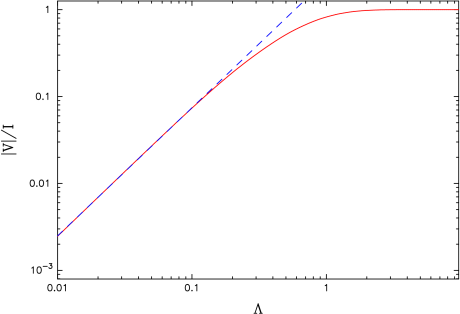
Figure 3: The final circular polarization fraction $|V|/I$ after wave mode coupling as a function of $\Lambda$ with the power-law index $n=3$. The linear polarization fraction before wave mode coupling is assumed to be $100\%$. The dash line depicts the fitting formula [eq. (4.77)] for $\Lambda<0.1$.

4.3 Circularization

Circularization happens when $|\beta_{\rm pol}|\sim 1$, and we can define the radius of circularization $r_{\rm cir}$ by $|\beta_{\rm pol}(r=r_{\rm cir})|=1$. For $r\gg r_{\rm cir}$, the normal modes become circular-polarized.

According to eq. (3.35), if $r_{\rm cir}\ll r_{\rm cyc}$ (or $\lambda\gg 1$, before cyclotron resonance) and $\theta_{B}\gamma\gg 1$, the polarization parameter

$$|\beta_{\rm pol}|\simeq\frac{\lambda}{\theta_{B}^{2}\gamma^{2}\Delta N/N-\Delta\gamma/\gamma}\gg 1,$$ (4.78)

which means the two wave modes are always linear polarized. However, if $r_{\rm cir}\ll r_{\rm cyc}$ and $\theta_{B}\gamma\ll 1$,

$$|\beta_{\rm pol}|\simeq\frac{\lambda\theta_{B}^{2}\gamma^{2}}{\Delta N/N-\Delta\gamma/\gamma},$$ (4.79)

so circularization could happen when

$$\theta_{B}\gamma=\sqrt{(\Delta N/N-\Delta\gamma/\gamma)/\lambda}.$$ (4.80)

Which implies a very small $\theta_{B}$. This condition could be satisfied when the photon ray is nearly aligned with the magenetic field, or when the photon is generated inside the $1/\gamma$ cone of the radiation beam.

If the circularization happens after the cyclotron resonance ($r_{\rm cir}\gg r_{\rm cyc}$ or $\lambda\ll 1$), according to eq. (3.36), the radius of circularization is given by

$$r_{\rm cir}/R_{\ast}=2.2\times 10^{3}B_{\ast 12}^{1/3}\nu_{9}^{-1/3}\theta_{B}^{-4/3}\gamma^{-1/3}(\Delta N/N-\Delta\gamma/\gamma)^{-1/3}.$$ (4.81)

Here we used $B\simeq B_{\ast}(r/R_{\ast})^{-3}$ and assumed $\theta_{B}\gamma\gg 1$. The ratio of $r_{\rm cir}$ and the cyclotron resonance radius [see eq. (4.49)] is

$$r_{\rm cir}/r_{\rm cyc}=1.2~{}\theta_{B}^{-2/3}(\Delta N/N-\Delta\gamma/\gamma)^{-1/3}\gg 1.$$ (4.82)

Obviously, in the parameter regions we interested in, the circularization radius is typically larger than the cyclotron resonance radius and the polarization limiting radius. Thus, this effect does not change the photon polarization state at all.

4.4 Quasi-Tangential Propagation Effect

In their study of the X-ray polarization signals from magnetized neutron stars, Wang & Lai (2009) found that as the X-ray photon travels through the magnetosphere, it may cross the region where its wave vector is aligned or nearly aligned with the magnetic field (i.e., $\theta_{B}$ is zero or small). In such a Quasi-Tangential region (QT region), the azimuthal angle of magnetic field $\phi_{B}$ changes quickly, the two photon modes ($\parallel$ and $\perp$ modes) become (nearly) identical, and mode coupling may occur, thereby affecting the polarization alignment. This Quasi-tangential Effect generally happens at a few $R_{\ast}$ for surface X-ray emission. The physical mechanism is similar to the wave mode coupling effect discussed in section 4.2 [see the mode evolution equation (2.11) in Wang & Lai (2009)], except that the magnetic field plays an important role.

In the radio case, we assume the photon is emitted in the tangential direction of the magnetic field line at the emission point ($\sim 50R_{\ast}$). If the NS is non-rotating, then the ${\mn@boldsymbol{k}}-\mn@boldsymbol{B}$ angle $\theta_{B}$ ($=0$ at the emission point) will increase monotonically and no QT effect will occur. However, when we consider the rotation of the NS, for some special photons (for example, those with small impact angle $\chi$ and special $\Psi_{\rm i}$) $\theta_{B}$ could attain its minimum value at a large radius. As an example, the two bottom panels of Figure 6 and 7 (to be discussed in detail in section 5) shows the evolution of $\theta_{B}$, $\phi_{B}$ along the ray for $\chi=0.5^{o}$. We see that $\theta_{B}$ reaches its minimum value at about $s=700R_{\ast}$ away from the emission point. The azimuthal angle $\phi_{B}$ changes very quickly at this radius. The two linear modes strongly couple with each other. The final polarization state after crossing this QT region is complicated: $\phi_{\rm PA}$ can be modified significantly and different sign of circular polarization can be generated for different geometry, which is different from wave mode coupling effect discussed in section 4.2. In general, the QT effect strongly influence the polarization phase profiles when impact angle is very small (see section 5.3). In our case, the QT effect is always coupled with wave mode coupling effect (occurring at almost same place), and the numerical ray integration is necessary to account for these effects accurately (see section 5).

5 Numerical Results

In section 4 we have discussed various key physical effects related to wave propagation through the magnetosphere. However, in many cases these different effects are coupled and not easy to separate. Thus, to produced the observed polarization profiles, it is necessary to use the numerical ray integrations to calculate the final wave polarization states.

5.1 Single Ray evolution

It is generally accepted that pulsar radio emission is emitted from the open field line region at a few to tens of NS radii (e.g. Cordes 1978; Blaskiewicz et al. 1991; Kramer et al. 1997; Kijak & Gil 2003). In this paper, we choose the emission height $r_{\rm em}=50R_{\ast}$ and assume that at the emission point, the photon is polarized in the ${\mn@boldsymbol{k}}$-$\mn@boldsymbol{B}$ plane (or the O-mode, as in the case of curvature radiation), and propagates along the tangential direction of the local magnetic field line (here we do not consider the emission cone of angle $1/\gamma$). For a given emission height $r_{\rm em}$, the pulsar rotation phase $\Psi_{i}$, the direction of line of sight $\zeta$ (which is the ${\mn@boldsymbol{k}}$-$\mn@boldsymbol{\Omega}$ angle), the surface magnetic field $B_{\ast}$, and the plasma properties (plasma density parameter $\eta$, Lorentz factor of the streaming plasma $\gamma$), we can calculate the dielectric tensor at each point along the photon ray, and integrate the wave evolution equation (2.10) from the emission point to a large radius (generally we choose $r_{\rm lc}/2$), beyond the polarization limiting radius $r_{\rm pl}$ and cyclotron resonance radius $r_{\rm cyc}$, to determine the final polarization state of the photon.

5.1.1 Symmetric pair plasma

We first consider the case of symmetric pair plasmas, i.e., the electrons and positrons have the same Lorentz factors ($\gamma_{p}=\gamma_{e}$, or $\Delta\gamma/\gamma=0$) and densities ($\Delta N/N=0$). In this case, the eigenmodes are always linear polarized (mixing angle $\theta_{m}=0^{o}$ or $90^{o}$). Figure 4 shows an example of the photon polarization evolution along its trajectory. We can clearly find the wave mode coupling effect (at $r_{\rm pl}\sim$ 800 $R_{\ast}$) and cyclotron absorption effect (at $r_{\rm cyc}$ more than 1000$R_{\ast}$). The final polarization position angle $\phi_{\rm PA}$ is determined by $\phi_{B}(r_{\rm pl})$ [see eq. (5.87)]. It is obvious that near the polarization limiting radius, $\Gamma_{\rm ad}\propto(r/r_{\rm pl})^{-n}$ and $n\sim 3$, so that as discussed in section 4.2, the final circular polarization is determined by the value of $\Lambda$ [see eq. (4.77)]. Since we are dealing with a symmetric pair plasma here, cyclotron absorptions do not change the polarization state (but decrease the total intensity).

Figure 5 give some other examples of the evolution of Stokes parameters with different plasma density $\eta$ and Lorentz factor $\gamma$. Different $\eta$ and $\gamma$ correspond to different $r_{\rm pl}$ [according to eq. (4.72), lower $\eta$ and higher $\gamma$ corresponds to a smaller $r_{\rm pl}$], so that the final $\phi_{\rm PA}$ is different too. In all the above cases, the final polarization state changes significantly compared to the original state, not only the linear position angle but also the circular polarization.

At the special parameter region of the initial rotation phase $\Psi_{\rm i}$, the QT effect (see section 4.4) can strongly affect the final polarization state. Figure 6 shows the photon evolution for $\Psi_{\rm i}=-9^{o}$ (the other parameters are the sames as in Fig. 4, e.g. the impact angle $\chi=2^{o}$). Note that in contrast to Fig. 4, here the ${\mn@boldsymbol{k}}-\mn@boldsymbol{B}$ angle $\theta_{B}$ does not vary monotonically along the ray. There exists a QT region around $s\sim 700R_{\ast}$, where $\theta_{B}$ is minimum and $\phi_{B}$ is changing very quickly. As discussed in section 4.4, the final $\phi_{\rm PA}$ and circular polarization are different from the prediction of pure wave mode coupling effect (which is the case in Fig. 4 where QT effect does not occur). For the photon evolution with a smaller photon impact angle $\chi=0.5^{o}$ (but the initial rotation phase and other parameters are the same as in Fig. 6), the QT effect is stronger, as shown in Figure 7. Note that even the sign of the final circular polarization in this figure is positive, as a result of the strong QT effect.

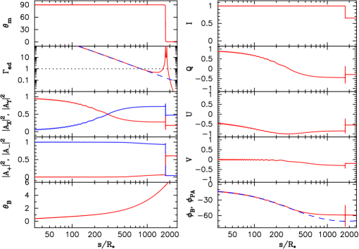
Figure 4: An typical single photon evolution across the magnetosphere. The horizontal axis $s/R_{*}$ is the photon distance away from the emission point. On the left panels, $\theta_{\rm m}$ is the mode mixing angle defined by eq. (3.37), $\Gamma_{\rm ad}$ is the adiabatic parameter defined by eq. (4.70) (the dashed line is the power-law fit of $\Gamma_{\rm ad}$ around $r_{\rm pl}$, which is $\Gamma_{\rm ad}\propto s^{-2.39}$), $A_{X}$ and $A_{Y}$ are the wave amplitudes in the fixed $XYZ$ frame. $A_{+}$ and $A_{-}$ are the mode amplitudes, and $\theta_{B}$ is the angle between ${\mn@boldsymbol{k}}$ and $\mn@boldsymbol{B}$. On the right panels, $I$, $Q$, $U$, $V$ are the Stokes parameters, $\phi_{\rm PA}=0.5\tan^{-1}(U/Q)$ is the linear polarization position angle (solid line) and $\phi_{B}$ is the azimuthal angle of the $\mn@boldsymbol{B}$ field (dashed line). The initial polarization is assumed to be in the ordinary mode, with $A_{+}=1$, $A_{-}=0$. For this example, the parameters are: surface magnetic field $B_{\ast}=10^{12}$ G, NS spin period $P=1$ s, wave frequency $\nu=1$ GHz, plasma density parameter $\eta=N/N_{\rm GJ}=400$ ($N=N_{e}+N_{p}$ and $N_{e}=N_{p}$), Lorentz factor $\gamma=100$ (with $\Delta\gamma/\gamma\simeq 0$), inclination angle $\alpha=30^{o}$, impact angle $\chi=2^{o}$, initial rotation phase $\Psi_{\rm i}=0^{o}$, and emission height $r_{\rm em}=50R_{\ast}$.

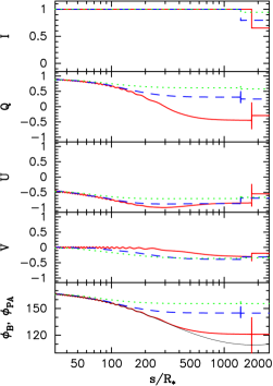
Figure 5: Same as the right panels of Fig. 4, except for different plasma density $\eta$ and Lorentz factor of the streaming motion $\gamma$: the solid lines are for $\eta=400$, $\gamma=100$ (same as Fig. 4), the dashed lines for $\eta=400$, $\gamma=300$ and the dotted lines for $\eta=100$, $\gamma=100$. The thin line in the bottom panel is for $\phi_{B}$. It is obvious that for lower density and/or higher $\gamma$, the wave mode coupling occurs at smaller $r_{\rm pl}$.

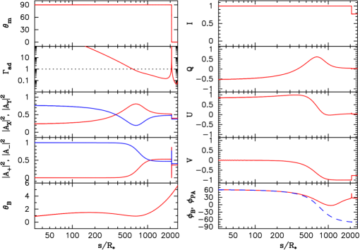
Figure 6: Same as Fig. 4, except for a different initial rotation phase $\Psi_{\rm i}=-9^{o}$. The impact angle is the same as in Fig. 4, $\chi=2^{o}$. Note that in contrast to Fig. 4, here the ${\mn@boldsymbol{k}}-\mn@boldsymbol{B}$ angle $\theta_{B}$ does not vary monotonically along the ray. There exists a quasi-tangential (QT) region around $s\sim 700R_{\ast}$, where $\theta_{B}$ is minimum and $\phi_{B}$ changes very quickly. Strong circular polarization is generated here and the final PA angle $\phi_{\rm PA}$ can not be predicted by simply using eq. (5.84).

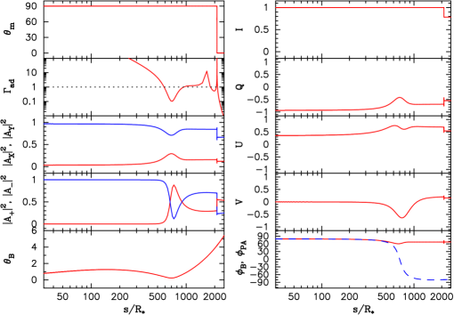
Figure 7: Same as Fig. 6, except for the impact angle $\chi=0.5^{o}$. The very smaller impact angle makes $\phi_{B}$ change more quickly around $s\sim 700R_{\ast}$, so that the QT effect is stronger than the case shown in Fig. 6. Note that the sign of final circular polarization is different from the cases in Fig. 4 and 6.

5.1.2 Asymmetric pair plasma

If the electrons and positrons of the magnetospheric plasma have different velocities and/or densities, the wave eigenmodes cannot always be linearly polarized. As discussed in section 4.3, before cyclotron resonance the natural modes are linearly polarized [see eq. (4.78)] for $\theta_{B}\gamma\gg 1$. After the cyclotron resonance, the natural modes become elliptical polarized. In section 4.3, we have defined a circularization radius $r_{\rm cir}$ where the polarization parameter $|\beta_{\rm pol}|=1$ [see eqs. (4.81) and (4.82)]. For $r\gg r_{\rm cir}$, the natural modes becomes circular polarized.

According to eq. (4.73), for typical plasma parameters of interest in this paper, $\eta\mathrel{\raise 1.29167pt\hbox{$>$}\mkern-14.0mu\lower 2.58334pt\hbox{$\sim$}}100$ and $\gamma\mathrel{\raise 1.29167pt\hbox{$>$}\mkern-14.0mu\lower 2.58334pt\hbox{$\sim$}}100$, wave mode coupling always occurs before the cyclotron resonance ($r_{\rm pl}<r_{\rm cyc}$). Thus, circularization always happens after wave mode coupling, at which point the wave polarization state is already frozen. Therefore the change of natural mode does not affect the observed polarization state. Figure 8 shows the photon evolution in an asymmetric pair plasma. Note that the mode mixing angle $\theta_{m}$ changes from $0^{o}/90^{o}$ to $45^{o}$ after the cyclotron resonance, but the polarization state does not change since $r_{\rm cir}>r_{\rm pl}$.

von Hoensbroech et al. (1998) studied wave modes in a pure electron plasma. They assumed that the background plasma has a much lower Lorentz factor (e.g. $\gamma_{\rm bg}=1.7$) than the Lorentz factor of the radiating beam. In this case $r_{\rm cir}$ may be close to $r_{\rm pl}$ and circular polarization may be generated around $r_{\rm cir}$. Note that they did not calculate $r_{\rm pl}$ but simply assumed that the final photon polarization is determined by the normal mode at some fixed $r_{\rm pl}$.

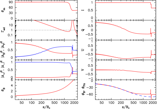
Figure 8: Same as Fig. 4, except for an asymmetric pair plasma with $\Delta\gamma/\gamma=0.2$, $\Delta N/N=0$. Since the Lorentz factors of electrons and positrons are different, their cyclotron resonance occur at different radii. Note that after the cyclotron resonance, the natural modes become circular polarized ($\theta_{m}=45^{o}$).

5.2 Polarization Profiles of Pulsar Emission Beam

Having understood the main features of polarization evolution along a single ray, we now proceed to calculate the polarization profiles of pulsar emission beam. To do this, one needs to know the emission height as a function of pulsar rotation phase. For simplicity, in this paper, we assume that all emissions are from the same height, at $r_{\rm em}=50R_{\ast}$, and defer the results for emissions from a range of heights to a future paper. For a given emission height $r_{\rm em}$, the pulsar rotation phase $\Psi_{i}$, the inclination angle $\alpha$ and the direction of line of sight $\zeta$ (which is the ${\mn@boldsymbol{k}}$-$\mn@boldsymbol{\Omega}$ angle), we can find the position of the emission point $\mn@boldsymbol{r}_{\rm i}$ where the tangential magnetic field line direction is along the line of sight. This emission point, $\mn@boldsymbol{r}_{\rm i}=(r_{\rm em},~{}\theta_{r{\rm i}},~{}\phi_{r{\rm i}})$, is given by (in the fixed $XYZ$ frame)

$$\theta_{r{\rm i}}=\frac{\theta_{\mu{\rm i}}}{2}-\frac{1}{2}\sin^{-1}\left(\frac{1}{3}\sin\theta_{\mu{\rm i}}\right),\quad~{}~{}\phi_{r{\rm i}}=\phi_{\mu{\rm i}},$$ (5.83)

where ($\theta_{\mu{\rm i}}$, $\phi_{\mu{\rm i}}$) is the initial direction of the dipole magnetic momentum $\mn@boldsymbol{\mu}_{i}$ and can be found in eq. (2.5) (with $\Psi$ given by $\Psi_{\rm i}$). We consider emissions only from the open field line region, i.e., the angle between $\mn@boldsymbol{r}_{\rm i}$ and $\mn@boldsymbol{\mu}_{\rm i}$ should be less than $\sqrt{r_{\rm em}/r_{\rm lc}}$.

For given $r_{\rm em}$, $\alpha$, $\zeta$, $\Psi_{i}$ and initial polarization state (ordinary mode), we determine $\mn@boldsymbol{r}_{\rm i}$ and calculate the final observed Stokes parameters by integrating along the ray. When the phase $\Psi_{i}$ varies due to NS rotation, we can observe photons from different emission points and the final observed Stokes parameters will change with the rotation phase — this is the pulsar polarization profile. If we neglect the propagation effect, the observed position angle $\phi_{\rm PA}$ can be described by the Rotating-Vector-Mode (RVM) (see Radhakrishnan & Cooke 1969) as

$$\phi_{\rm PA}=\phi_{\mu{\rm i}}=\phi_{\mu}(\Psi_{i})=\tan^{-1}\frac{-\sin\alpha\sin\Psi_{i}}{\sin\zeta\cos\alpha-\cos\zeta\sin\alpha\cos\Psi_{i}}.$$ (5.84)

The basic assumption of the RVM is that the radiation is emitted with polarization in the plane of the field line curvature (i.e. the ${\mn@boldsymbol{k}}$-$\mn@boldsymbol{B}$ plane) and this polarization direction is unchanged during the propagation. However, as seen in section 5.1, the final polarization state can be modified compared to the initial one because of the propagation effect in the magnetosphere, so that the final PA profile can deviate significantly from the RVM model.

Figure 9 shows a typical example of the phase evolution of the intensity and polarization, taking into account of all the propagation effects. The total intensity is only affected by cyclotron absorption, and a higher plasma density leads to stronger absorption. We see that the relative intensity $I/I_{0}$ varies with the rotation phase $\Psi_{\rm i}$, simply because the wave passes through different paths in the magnetosphere for different $\Psi_{\rm i}$. For illustrative purpose, we consider the initial intensity profile $I_{0}$, given by a Gaussian centered at $\Psi_{\rm i}=0$:

$$I_{0}(\Psi_{\rm i})=\exp(-4\sqrt{\ln 2}\Psi_{\rm i}^{2}/(\Psi_{\rm max}^{2})).$$ (5.85)

Here $\Psi_{\rm max}$ is the initial phase of the photon from the edge of the open field region and is given by

$$\cos\Psi_{\rm max}=\frac{\cos\theta_{\rm open}-\cos\zeta\cos\alpha}{\sin\zeta\sin\alpha}$$ (5.86)

where $\theta_{\rm open}\simeq\sqrt{r_{\rm em}/r_{\rm lc}}$ is the half-cone angle of the open field region at emission height $r_{\rm em}$ (here we simply assume the open field region is always the same as the $\mn@boldsymbol{\mu}\parallel\mn@boldsymbol{\Omega}$ case). Since $I/I_{0}$ depends asymmetrically on $\Psi_{i}$, the observed intensity $I$ is no longer a Gaussion. Non-gaussion profiles have been observed in many pulsars, and the phase-dependent cyclotron absorption illsutrated here is a possible explanation.

The final polarization profiles are also strongly affected by the propagation effects. When the plasma density is not so high, and/or the impact angle $\chi$ is not so small [compared to the half cone angle of the emission beam from the open field region $\theta_{\rm beam}$; e.g., in Fig. 9(a), $\chi=5^{o}$ while $\theta_{\rm beam}\simeq 1.5\theta_{\rm open}=8.8^{o}$], the wave mode coupling effect is not strong and the final circular polarization is not very high. In this case, the final linear polarization position angle is determined by the azimuthal angle of $\mn@boldsymbol{B}$ field at the polarization limiting radius $\phi_{B}(r_{\rm pl})$:

$$\phi_{\rm PA}\simeq\phi_{B}(r_{\rm pl})\simeq\pi+\phi_{\mu}(r_{\rm pl})=\pi+\phi_{\mu}(\Psi_{i}+r_{\rm pl}/r_{\rm lc}).$$ (5.87)

Here we have used the approximation of $\mn@boldsymbol{B}(\mn@boldsymbol{r})=-\mn@boldsymbol{\mu}/r^{3}$ since $r_{\rm pl}\gg R_{\ast}$. In general, the polarization limiting radius, $r_{\rm pl}$, does not vary significantly with different rotation phase $\Psi_{\rm i}$. Thus the final PA profile just shifts by the amount

$$r_{\rm pl}/r_{\rm lc}\simeq 0.08\left(\frac{\eta}{10^{3}}\right)^{1/3}\left(\frac{B}{10^{12}\,{\rm G}}\right)^{1/3}\left(\frac{\nu}{1\,{\rm GHz}}\right)^{-1/3}\left(\frac{\gamma}{10^{2}}\right)^{-1}\left(\frac{\theta_{B}}{0.1}\right)^{-2/3}\left(\frac{P}{1\,{\rm s}}\right)^{-1}\left(\frac{F_{\phi}}{10}\right)^{-1/3}$$ (5.88)

compared to the RVM model. The final circular polarization is always single sign in this case. We can easily find the relationship between $\phi_{\rm PA}$ and the sign of circular polarization. According to eq. (5.87), the monotonicity of the final PA angle $\phi_{\rm PA}(\Psi_{\rm i})$ is given by

$$\frac{{\rm d}\phi_{\rm PA}}{{\rm d}\Psi_{\rm i}}=\frac{{\rm d}\phi_{B}(r_{\rm pl})}{{\rm d}\Psi}\frac{{\rm d}\Psi}{{\rm d}\Psi_{\rm i}}=\frac{{\rm d}\phi_{B}(r_{\rm pl})}{{\rm d}\Psi}.$$ (5.89)

Here $\Psi=\Psi_{\rm i}+s/r_{\rm lc}$ [see eq. (2.2)], so that ${\rm d}\Psi/{\rm d}\Psi_{\rm i}=1$. The sign of the final circular polarization (generated by wave mode coupling effect) is determined by ${\rm d}\phi_{B}(r_{\rm pl})/{\rm d}s$ [$\phi_{B}^{\prime}$ in eq. (4.77)] and:

$$\frac{{\rm d}\phi_{B}(r_{\rm pl})}{{\rm d}s}=\frac{{\rm d}\phi_{B}(r_{\rm pl})}{{\rm d}\Psi}\frac{{\rm d}\Psi}{{\rm d}s}=\frac{{\rm d}\phi_{B}(r_{\rm pl})}{{\rm d}\Psi}\frac{1}{r_{\rm lc}}.$$ (5.90)

So that ${\rm d}\phi_{\rm PA}/{\rm d}\Psi_{\rm i}$ always has the same sign as ${\rm d}\phi_{B}(r_{\rm pl})/{\rm d}s$. According to eqs.  (4.77) and (5.90), we can find that because of the wave mode coupling effect, a monotonically increasing $\phi_{\rm PA}$ leads to a positive $V$ while a monotonically decreasing $\phi_{\rm PA}$ gives a negative $V$. This relationship has been observed in some conal-douple type pulsars; see section 5.3.

(a) $\chi=5^{o}$	(b) $\chi=2^{o}$

Figure 9: The intensity and polarization profiles computed by ray integrations. We use two different impact angles: (a) $\chi=5^{o}$ on the left panels, and (b) $\chi=2^{o}$ on the right panels. The solid lines are for plasma density parameter $\eta=10$, the dashed lines for $\eta=100$ and the dot-dashed line for $\eta=400$. The top panels show the total intensity profiles, where we have adopted (for illustrative purpose) a Gaussian initial intensity profile $I_{0}(\Psi_{\rm i})=\exp(-4\sqrt{\ln 2}\Psi_{\rm i}^{2}/\Psi_{\rm max}^{2}))$ (this initial profile is shown shown as dotted lines, almost coincident with the solid lines). The second panels form the top show the modification factor $I/I_{0}$ due to propagation effects. The bottom three panels show the linear polarization fraction $L/I$, circular polarization $V/I$ and the position angle of the LP, $\phi_{\rm PA}$. In the bottom panels, the dotted lines (almost coincident with the solid line on the left panel) show the prediction from the RVM model: $\phi_{\rm PA}=\phi_{\mu{\rm i}}\simeq\phi_{Bi}$. In these calculations, the initial polarization states are all ordinary mode, and the other parameters are: surface magnetic field $B_{\ast}=10^{12}$ G, NS spin period $P=1$ s, wave frequency $\nu=1$ GHz, Lorentz factor $\gamma=100$ (with $\Delta\gamma/\gamma\simeq 0$), inclination angle $\alpha=30^{o}$, and emission height $r_{\rm em}=50R_{\ast}$.

The polarization profiles can also be quite different from the RVM prediction, especially in the case of low impact angle and/or high plasma density. Figure 9(b) give some examples for the impact angle $\chi=2^{o}$. For the low density case of $\eta=10$, the final PA profile can still be approximated by a simple shift from the RVM model. However, for higher density ($\eta=200$, 400), the final PA profile is not just a simple shift compared with the RVM model. For example, the PA profile of $\eta=400$ case has a $90^{o}$ jump within $1^{o}$ around $\Psi_{i}\simeq-9^{o}$, where the linear polarization $L/I$ is close to 0 while the circular polarization $|V|/I$ reaches almost $100\%$. In this region the QT effect (discussed in section 4.4) plays an important role in determining the final polarization state (see Fig. 6).

5.3 Two-Dimensional Polarization Maps of Pulsar Emission Beam

For a given pulsar, observation at different line of sight (i.e., different $\zeta$ or impact angle $\chi$) would obviously result in different intensity and polarization profiles. Figure 10 gives an example of the two-dimensional polarization map of the observed Stokes parameters, produced by varying $\chi$ and $\Psi_{i}$, while keeping all other parameters fixed. As discussed before, the final total intensity $I$ is only affected by cyclotron absorption, while the linear and circular polarizations are modified by wave mode coupling effect and QT effect, and can deviate significantly from the prediction of RVM model. Figure 11 shows four profiles with four different impact angle $\chi$, corresponding to four sections of Fig. 10. These four sections represent three typical final polarization states produced by the propagation effects:

(i) For a relatively large impact angle $|\chi|$, the final PA profile can be obtained by a small shift from the RVM profile, of the amount $r_{\rm pl}/r_{\rm lc}$ [see eqs. (5.87) and (5.88)]. Figure 9 and the $\chi=-5^{o}$ column of Fig. 11 depict some examples. The final circular polarization is always of single sign: a monotonically increasing $\phi_{\rm PA}$ leads to a positive $V$ while a monotonically decreasing $\phi_{\rm PA}$ gives a negative $V$ [see eqs. (4.77) and (5.90)]. This behavior is consistent with observations of the double cone emission of some pulsars (“conal-double type pulsars”), where a correlation between the sense of CP and the sense of PA variation was found (see Han et al. 1998).

(ii) For relatively small impact angle, the final PA profile is very different from the RVM prediction – the middle two columns ($\chi=-1.9^{0}$ and $\chi=-1^{0}$) of Fig. 11) give some examples. It is clear that there always exists a special line of sight ($\chi=\chi_{\rm jump}$), for which the PA profile has a $90^{o}$ jump (where $Q=0$ while $U$ changes signs [see the $\chi=-1.9^{0}$ column of Fig. 11]. The large jumps in $V/I$ and $\phi_{\rm PA}$ are caused by the QT effect. For $|\chi|<\chi_{\rm jump}$, the PA is not necessarily an monotonic function of $\Psi_{i}$. Nevertheless, the final CP retains a single sign, which is the same as the case with large $|\chi|$.

(iii) For very small impact angle ($|\chi|\ll\chi_{\rm jump}$), the QT effect is much stronger, so that the final PA profile is very different from the prediction of RVM model and even the CP does not stay at a single sign (see the right-most column of Fig. 11).

The above three types of polarization behaviours always exist for different pulsar and plasma parameters (e.g., $B_{\ast}$, $P_{0}$, $\nu$, $\eta$, $\gamma$, $\alpha$ and $r_{\rm em}$). Different parameters just modify the position of $\chi_{\rm jump}$ and the initial rotation phase where the $90^{o}$ jump in PA occurs, while the basic morphology of the emission beam does not change.

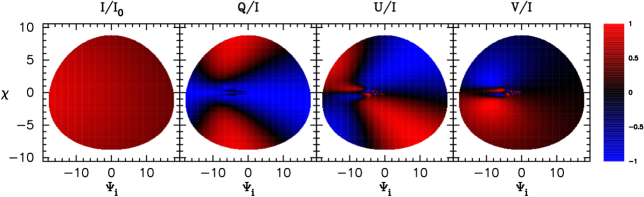
Figure 10: Two-dimensional polarization map of pulsar emission beam. The four panels correspond to the four Stokes parameters $I$, $Q/I$, $U/I$, $V/I$. The filled region is the emission beam from the open field region. The values of the four Stokes parameters are shown as different colors (with red for positive value while blue for negative). The map is obtained by computing the observed wave polarization for different impact angle $\chi$ (which varies from $-\theta_{\rm beam}$ to $\theta_{\rm beam}$, here $\theta_{\rm beam}\simeq 8.8^{o}$) and the rotation phase $\Psi_{i}$. The other (fixed) parameters are: surface magnetic field $B_{\ast}=10^{12}$ G, NS period $P=1$ s, wave frequency $\nu=1$ GHz, plasma density $\eta=N/N_{\rm GJ}=400$ ($N=N_{e}+N_{p}$ and $N_{e}=N_{p}$), Lorentz factor $\gamma=100$ (with $\Delta\gamma/\gamma\simeq 0$), inclination angle $\alpha=30^{o}$, and emission height $r_{\rm em}=50R_{\ast}$.

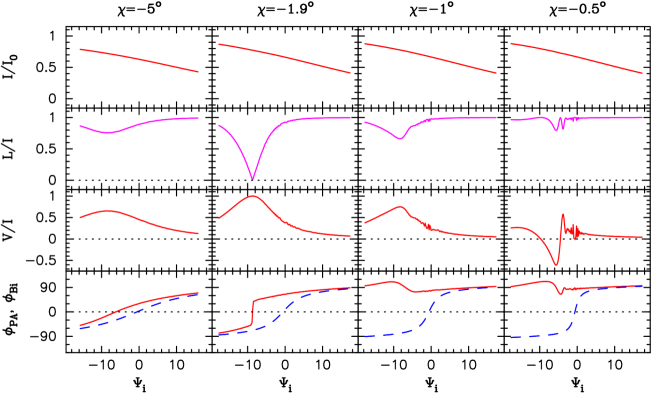
Figure 11: Intensity and polarization profiles of pulsar emission beam. The four columns correspond to four fixed impact angles $\chi=-5^{o}$, $-1.9^{o}$, $-1^{o}$ and $-0.5^{o}$, respectively, which are four sections in Fig. 10. In each column, we plot the Stokes parameters $I/I_{0}$ (top panel), $L/I$ (second panel), $V/I$ (third panel), $\phi_{\rm PA}$ and $\phi_{B\rm i}$ (bottom panel, the solid line for $\phi_{\rm PA}$ and the dashed for $\phi_{B\rm i}$). Note that there exists a $90^{o}$ jump of $\phi_{\rm PA}$ near $\Psi_{\rm i}=-9^{o}$ in the bottom panel of the $\chi=-1.9^{o}$ column. The other parameters are the same as in Fig. 10.

6 Conclusion and Discussion

We have studied the evolution of radio emission polarization in a rotating pulsar magnetosphere filled with relativistic streaming pair plasma. We quantify and compare the relative importance of several key propagation effects that can influence the observed radio polarization signals, including wave mode coupling, cyclotron absorption, propagation through quasi-tangential (QT) region, and mode circularization (due to asymmetric distributions of electrons and positrons). We use numerical integration of the photon polarization along the ray to incorporate all these propagation effects self-consistently within a single framework. We find that, for typical parameters of the magnetospheric plasma produced by pair cascade, and for an initially $100\%$ linear polarized radio wave, the final intensity and polarization position angle are modified by the propagation effects, and significant circular polarization can be generated.

We find that the most important propagation effects are cyclotron absorption, wave mode coupling and QT effect. Generally, cyclotron absorption occurs after the wave mode coupling [$r_{\rm cyc}>r_{\rm pl}$, see eq. (4.73)]. Thus, it only changes the total wave intensity and does not modify the wave polarization ($\phi_{\rm PA}$, $V/I$). For a large impact angle $|\chi|$ and/or relatively low plasma density, the final wave polarization angle $\phi_{\rm PA}$ is determined by the azimuthal angle of $\mn@boldsymbol{B}$ field at the polarization limiting radius $r_{\rm pl}$, and the observed circular polarization is determined by the value of $\Lambda=r_{\rm pl}\phi_{B}^{\prime}$ at $r=r_{\rm pl}$ [see eqs. (4.76) – (4.77)]. In this case, the observed $\phi_{\rm PA}$ profile is similar to the prediction of the Rotating-Vector Model (RVM), except for a phase shift by the amount $r_{\rm pl}/r_{\rm lc}$ [see eq. (5.88)]; the circular polarization has a single sign across the emission beam (see Fig. 9). For a small impact angle and/or high plasma density, the QT effect becomes important, the final polarization profiles are more irregular: a $90^{o}$ sudden jump in PA may occur at certain phase, accompanied by large circular polarization. For very small $|\chi|$, the circular polarization may change signs for at different phases (see the right column of Fig. 11).

In this paper, we have adopted the simplest (and minimum) assumptions about the property of the magnetospheric plasma and the intrinsic radio emission mechanism (see below). Nevertheless, our results already show great promise in explaining a number of otherwise puzzling observations:
(i) It has been observed that in some single-pulse pulsars, the intensity profile deviates from the single guassion shape. One possible reason is that cyclotron absorption depends on the rotation phase (because the ray passes through different region of the magnetosphere), as discussed in section 5.2. Thus, even when the initial intensity profile from the emission beam is a Gaussion, the observed profile can be non-gaussion.
(ii) For the so-called conal double type pulsars, which in our model corresponds to large impact angle $\chi$, the relationship between the single sign of the circular polarization and the derivation of $\phi_{\rm PA}$ (see Han et al. 1998) can be easily understood by the wave mode coupling effect. According to eqs. (4.77) and (5.90), an increasing $\phi_{\rm PA}$ corresponds to the left-hand circular polarization ($V>0$) while a decreasing $\phi_{\rm PA}$ corresponds to the right-hand ($V<0$) one .
(iii) According to our calculation, there exists a special impact angle $\chi_{\rm jump}$, where the observed $\phi_{\rm PA}$ profile has a $90^{o}$ jump (orthogonal polarization mode) and this is accompanied by the maximum circular polarization. This feature may be helpful to explain the polarization profile of PSR J1920+2650 (Figure 12; see Han et al. 2009). (iv) For a very small impact angle, which corresponds to the core emission, the QT effect can cause the sign reversal of circular polarization, which is observed in the core components of many pulsars (e.g. Radhakrishnan & Rankin 1990; Han et al. 1998; You et al. 2006).

Our calculations in this paper have relied on several simplifying assumptions. For example, we have assumed that the radio emission is from the same height for different rotation phases, that the density parameter ($\eta=N/N_{\rm GJ}$) of the magnetospheric plasma is constant everywhere in the emission cone and along the photon trajectory, and that the plasma electrons and positrons have the same for bulk Lorentz factors. In future works, we plan to consider models with varying emission heights, as well as non-trivial electron/positron spatial and velocity distributions. We did not include the small but finite emission cone (angle $1/\gamma$) in our model, and assumed that the initial polarization of photon is always O-mode for different rotation phases. However, different emission mechanisms could give different initial polarization states. We will also be interested in studying the propagation effects on the individual/subpluse emissions, since they may more directly reflect the underlying radio emission processes.

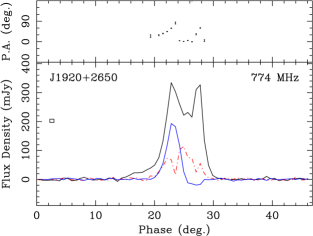
Figure 12: Intensity and polarization profiles of PSR J1920+2650. In the lower panel, the upper thick line is the total intensity ($I$), the dash-dot-dashed line is the linear polarized intensity $L$, and the thin line is the circularly polarized intensity $V$. This pulsar shows extremely strong circular polarization with $V/I\simeq 64\%$ in its first major component.

References

- [] Allen, M. C. & Melrose, D. B. 1982, PASAu, 4, 365
- [] Arons, J. & Barnard, J. J. 1986, ApJ, 302, 120
- [] Backer, D. C.; Rankin, J. M.; Campbell, D. B. 1976, Nature, 263, 202
- [] Barnard, J. J. & Arons, J. 1986, ApJ, 302, 138
- [] Beloborodov, A. M. & Thompson, C. 2007, ApJ, 657, 967
- [] Blandford, R. D. & Scharlemann, E. T. 1976, MNRAS, 174, 59
- [] Blaskiewicz, M., Cordes, J. M. & Wasserman, I. 1991, ApJ, 370, 643
- [] Cheng, A. F. & Ruderman, M. A. 1979, ApJ, 229, 348
- [] Cognard, I.; Shrauner, J. A.; Taylor, J. H. & Thorsett, S. E. 1996, ApJ, 457, 81
- [] Cordes, J. M. 1978, ApJ, 222, 1006
- [] Cordes, J. M.; Rankin, J. & Backer, D. C. 1978, ApJ, 223, 961
- [] Daugherty, J. K. & Harding, A. K. 1982, ApJ, 252, 337
- [] Fussell, D., Luo, Q. & Melrose, D. B. 2003, MNRAS, 343, 1248
- [] Gould, D. M. & Lyne, A. G. 1998, MNRAS, 301, 235
- [] Han, J. L., Demorest, P. B., van Straten, W. & Lyne, A. G. 2009, ApJS, 181, 557
- [] Han, J. L.; Manchester, R. N.; Xu, R. X. & Qiao, G. J. 1998, MNRAS, 300, 373
- [] Hibschman, J. A. & Arons, J. 2001, ApJ, 554, 624
- [] Johnston, S., Ball, L., Wang, N. & Manchester, R. N. 2005, MNRAS, 358, 1069
- [] Kazbegi, A. Z., Machabeli, G. Z. & Melikidze, G. I. 1991, MNRAS, 253, 377
- [] Kijak, J. & Gil, J. 2003, A&A, 397, 969
- [] Kramer, M., Xilouris, K. M., Jessner, A., Lorimer, D. R., Wielebinski, R.& Lyne, A. G., 1997, A&A, 322, 846
- [] Lai, D. & Ho, W. C. G. 2003, ApJ, 588, 962
- [] Lai, D. & Ho, W. C. G. 2002, ApJ, 566, 373
- [] Luo, Q. H. & Melrose, D. B., 2004, in Camilo F., Gaensler B. M., eds, Proc. IAU Symp. 218, Young Neutron Stars and Their Environments. Astron. Soc. Pac., San Francisco, p. 381
- [] Luo, Q. H. & Melrose, D. B. 2001, MNRAS, 325, 187
- [] Lyne, A. G. & Manchester, R. N. 1988, MNRAS, 234, 477
- [] Lyubarsky, Y. 2008, in 40 YEARS OF PULSARS, eds. C. Bassa, Z. Wang, A. Cumming, & V. M. Kaspi, AIP Conf. Ser., 983, 29
- [] Lyubarskii, Y. E. & Petrova, S. A., 1998, Ap&SS, 262, 379
- [] Manchester, R. N.; Taylor, J. H.; Huguenin, G. R. 1975, ApJ, 196, 83
- [] McKinnon, Mark M. & Stinebring, Daniel R. 2000, ApJ, 529, 435
- [] Medin, Z. & Lai, D. 2009, submitted to MNRAS
- [] Melrose, D. B. 2003, in Radio Pulsars, eds. M. Bailes, D. J. Nice, & S. E. Thorsett, AIP Conf. Ser., 302, 179
- [] Melrose, D. B. 1979, AuJPh, 32, 61
- [] Mitra, D. & Li, X. H. 2004, A&A, 421, 215
- [] Petrova, S. A. 2006, MNRAS, 366, 1539
- [] Petrova, S. A. & Lyubarskii, Y. E. 2000, A&A, 355, 1168
- [] Radhakrishnan, V. & Cooke, D. J. 1969, ApJ, 3, 225
- [] Radhakrishnan, V. & Rankin, J. M. 1990, ApJ, 352, 258
- [] Rafikov, R. R. & Goldreich, P. 2005, ApJ, 631, 488
- [] Rankin, J. M. 1983, ApJ, 274, 333
- [] Stinebring, D. R., Cordes, J. M., Rankin, J. M., Weisberg, J. M., & Boriakoff, V. 1984a, ApJS, 55, 247
- [] Stinebring, D. R., Cordes, J. M., Weisberg, J. M., Rankin, J. M., & Boriakoff, V. 1984b, ApJS, 55, 279
- [] Thompson, C., Lyutikov, M., & Kulkarni, S. R. 2002, ApJ, 574, 332
- [] van Adelsberg, M. & Lai, D. 2006, MNRAS, 373, 1495
- [] van Hoensbroech, A., Lesch, H. & Kunzl, T. 1998, A&, 336, 209
- [] Wang, C. & Lai, D. 2007, MNRAS, 377, 1095
- [] Wang, C. & Lai, D. 2009, MNRAS, 398, 515
- [] Weisberg, J. M., Cordes, J. M., Kuan, B., Devine, K. E., Green, J. T. & Backer, D. C. 2004, ApJS, 150, 317
- [] Weisberg, J. M., Cordes, J. M., Lundgren, S. C., Dawson, B. R., Despotes, J. T., Morgan, J. J., Weitz, K. A., Zink, E. C. & Backer, D. C. 1999, ApJS, 121, 171
- [] Xilouris, K. M.; Seiradakis, J. H.; Gil, J.; Sieber, W. & Wielebinski, R. 1995, A&A, 293, 153
- [] Xu, R. X., Liu, J. F., Han, J. L. & Qiao, G. J. 2000, ApJ, 535, 354
- [] You, X. P. & Han, J. L. 2006, ChJAA, 6, 237