Emission coordinates for the navigation in space

Abstract

A general approach to the problem of positioning by means of pulsars or other pulsating sources located at infinity is described. The counting of the pulses for a set of different sources whose positions in the sky and periods are assumed to be known, is used to provide null emission, or light, coordinates for the receiver. The measurement of the proper time intervals between successive arrivals of the signals from the various sources is used to give the final localization of the receiver, within an accuracy controlled by the precision of the onboard clock. The deviation from the flat case is discussed, separately considering the different possible causes: local gravitational potential, finiteness of the distance of the source, proper motion of the source, period decay, proper acceleration due to non-gravitational forces. Calculations turn out to be simple and the result is highly positive. The method can also be applied to a constellation of satellites orbiting the Earth.

1 Introduction 

An extremely important problem posed by the needs of navigation through space and also of movement on the surface of the Earth and close to it, is the one of positioning with respect to some appropriate global reference system. Presently this problem is dealt mostly using GPS. Analogous systems are GLONASS and in the next future the European Galileo system (as well as others partially deployed or under implementation). All these systems were initially developed for military purposes, and, in the case of both GPS and GLONASS, they are still under primary military control. The basic idea there, is quite traditional: if we are able to measure the times of flight of electromagnetic signals arriving from a set of at least three sources occupying known positions, then we can, by means of a triangulation process, work out the position of the receiver in the same reference frame as the sources. This approach requires a common global time reference and implies the emitters to be synchronized with each other and with the user. If the sources are at least four, you may, in principle, dispense with the clock of the receiver. In practice a rapidly converging trial and error approach is used and a clock at the reception point is also needed. As it is also well known, GPS treats the relativistic aspects of the positioning as perturbations to a basic Newtonian method [1][2]. If relativity were neglected the positioning error would turn out to be huge and unacceptable. The special relativistic effects (influence of the speed of the satellites and Sagnac effect) and the general relativistic ones (blue shift of the flying clocks with respect to the ones on the ground) are separately introduced as corrections. Here we shall expound the essentials of a positioning system developed from scratch on fully relativistic bases and using the very space-time as the actual fiducial frame. As we shall see we describe our approach considering the pulsars as sources, even though the method is applicable to the case of freely falling clocks in the terrestrial environment (satellites) also. The idea of using pulsars as clocks has been considered almost from the year of their discovery. It has been discussed in various ways because it is appealing, however there are technological limitations which make things difficult. The point is mainly that the signals from pulsars are very weak, so that, usually, sophisticated and large sized devices (radiotelescopes) are needed. To avoid the inconvenience of the dimensions of the antenna, X-ray pulsars have also been envisaged [3]: the number of sources is not that big and the signals are weak too, however the noise is comparatively small also. In our case we shall consider millisecond pulsars where unfortunately the signal to noise ratio is really unfavorable. We thought however that comparatively large antennas could be allowed for space missions. In any case we are not treating here the technology problems. We have developed a computation method and a reasonably simple (much simpler than the present GPS method) algorithm to convert the arrival times of the signals from the pulsars into practical coordinates of a reference frame at rest with the ”fixed” stars. As we shall see, our method includes the effects of the gravitational field and allows a spacecraft to know what its absolute motion is with an accuracy controlled by the precision of the clock it carries, making it independent from control from the ground.

2
Pulsars

I am here very shortly reviewing pulsars and their features. Pulsars are neutron stars generated at the moment of the implosion of the core of a collapsing star in a supernova event. The pulsar possesses a very high magnetic field whose axis is in general not aligned with the spin axis of the star. Matter from an accretion disk, falling towards the surface of the pulsar, is ionized, then expelled, in the form of charged particles, along the lines of the magnetic field. The particles flux is accompanied by a highly collimated beam of electromagnetic radiation. Due to the misalignment of the magnetic field and the rotation axis of the star, the beam behaves as the radiation from a lighthouse. When we are in an appropriate position for seeing it, it reaches us one time per revolution of the star. The neutron star is spun at very high angular speeds by the conservation of angular momentum during the collapse. The rotation period of the pulsar coincides with the return time of the pulses. The period of the known pulsars ranges from the scale of the millisecond up to several seconds and slowly decays in time, due to rotational energy loss by the star. The behaviour of the objects under observation since years is very well known. Even though the time profile of each single pulse is usually different from the others, pulsars may be thought of as extremely stable clocks whose accuracy is overcome only by the best modern atomic clocks. In the long term however pulsars always carry the day. This is the reason why these objects can be considered as interesting celestial beacons. The known pulsars so far are approximately 1800 and are all located in our galaxy (apart from a handful of X-rays emitting objects in the Magellanic clouds), usually within a few thousands of light years from the Earth. Many of the stars are in binary systems, however we shall focus on isolated millisecond pulsars. Isolated objects may reasonably be considered as ”fixed stars” since their proper motions in the sky show up only on rather long periods of time.

3
Emission coordinates

In a relativistic framework, space and time are compound together in a four-dimensional manifold endowed with geometrical properties. The gravitational field is accounted for as a curvature in the manifold. In order to localize ”events” (points in space-time) four independent numbers (coordinates) are needed. These may of course be, for example, three Cartesian coordinates and one time, but any quadruple of independent parameters would fit as well. Consider now four independent clocks. Suppose, for simplicity, they are in free fall (geodetic motion) and that they broadcast their own time (their proper time). An observer who receives the signals from the four emitters gets, at any moment, the information concerning the proper emission time of the perceived signal from each source. The quadruple of these times depends on the space-time position of the receivers; each quadruple is uniquely associated with each event. This means that the four times conveyed by the electromagnetic signals are indeed a good set of coordinates for identifying positions in space and time. It is also clear now why these coordinates are called emission coordinates. Their use has been analyzed and proposed by various authors [4][5][6][7][8].

4
Basic frame

Suppose now to have a number ($\geq 4$) of sources of electromagnetic pulsed signals located at infinity and at rest with respect to each other. Let us assume also that our space-time is flat (Minkowski space-time). In these conditions the four-dimensional trajectories of electromagnetic signals, as well as of freely falling objects (inertial observers) are straight lines. Each one of our sources is characterized by the frequency of its pulses and by their direction in space. In a relativistic description this information is contained in a four- vector, tangent to the space-time trajectory (world-line) of the light rays. The four-vector of the $a$-th source may be written as

$$\chi_{a}=\frac{2\pi}{T_{a}}(1,\hat{n}_{a})$$

where $T_{a}$ is the period of the pulsar and $\hat{n}$ is a unit ordinary vector in space (three-vector) whose components are the direction cosines in any given reference frame. In relativity $\chi_{a}$ is the wave four-vector of the electromagnetic signal from source $a$ and is a null vector because it is self-orthogonal, i.e. the scalar product by itself is zero

$$\chi_{a}^{2}=\chi_{a}\cdot\chi_{a}=0$$ (1)

Under the general conditions we have chosen the wave vector from each source is fixed (the same everywhere and at all times). If we wish to localize an event with respect to an arbitrary origin, we may think to draw a radius four-vector from the origin to the given event. In four, as well as in three, dimensions a vector is characterized by its components with respect to some basis. In our case we can choose as basis vectors four neither collinear nor coplanar wave vectors from different sources. This will be a typical null basis, so called because of the nature of its elements [9]. The components of the position four-vector with respect to this basis will be called the null coordinates of the given event. We may associate to each of the new basis vectors (which essentially marks a direction in space-time) a family of conjugate three-dimensional hypersurfaces proceeding more or less as we would do in three dimensions. In this case we get a family of parallel null hyperplanes filling up the whole space-time. In three dimensions one would obtain the wave fronts and the concept may safely be extended to four dimensions. We then may single out the set of hyperplanes that represent the wave fronts of the corresponding pulses and label them by the ordinal numbers counted from an arbitrary origin. Finally we cover the whole space-time with a grid made of the fiducial hyperplanes. The situation is sketched in figure 1.

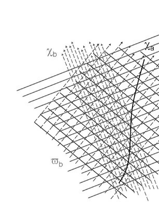
Figure 1: An example of the grid mapping, in this case, a flat 1+1 dimensional manifold. Vertically there is time, horizontally space. Dashed lines are worldlines of electromagnetic signals; the arrows show the directions of the null wavevectors $\chi_{a}$ and $\chi_{b}$. The symbols $\varpi_{a,b}$ label the two families of hyperplanes corresponding to the wavefronts. Each wavefront is associated with an integer number; the knots in the resulting grid are identified by a pair of integers: their null coordinates. The continuous wavy line represents the world-line of an observer.

Considering now a receiver able to recognize and count the signals coming from the various sources, the ordinal numbers used to label the subsequent pulses will naturally be a set of null coordinates using the $\chi$ vectors as their basis and having a single value over each specific null hypersurface. Introducing the periods of each source, the position four-vector of an event may then be written as

$$r=[(n+x)T]^{a}\chi_{a}$$ (2)

The Einstein convention has been used; $n$ is an integer and $x$ a fractional number, usually ranging from 0 to 1, even though, as we shall see, it will be allowed to assume values bigger than 1.

In practice, considering the dimensions and the definition of $\chi$, the components of the position four-vector coincide with the phases of the waves reaching the event from the various sources. The phase has the same value over any given hypersurface.

While travelling through space-time (see fig.1) an observer “crosses” successive hyperplanes and can count the crossing events (arrival of the pulses). The start (the $0$) of the reckoning will be arbitrarily chosen in correspondence of the arrival of, say, a signal from source $a$, then the $0$ for source $b$ will be the first $b$ pulse arriving after the $0$ of $a$, etc… If the receiver carries its own clock, this can be used to measure the proper time span between the arrival times from the various sources. In practice the receiver will be able to reconstruct its own world-line with respect to the infinitely far away sources and the arbitrarily chosen origin. We have implicitly assumed that the frequencies of the pulses from the basis sources are not too different from each other and the best choice would be to use the smallest one as the reference (the $a$-th source). As said, the families of hyperplanes build a space-time coordinated grid; the knots of the grid are identified by quadruples of integer numbers.

A general event will of course not coincide with any of the knots of the grid, but will be contained within a four-volume whose size, expressed in metrical units, will be

$$\Delta V=\frac{c^{2}}{4!}\varepsilon^{abcd}\left(T^{2}\chi\right)_{a}\wedge\left(T^{2}\chi\right)_{b}\wedge\left(T^{2}\chi\right)_{c}\wedge\left(T^{2}\chi\right)_{d}$$ (3)

The compact mathematical notation of eq. (3) introduces the speed of light $c$ and the completely anti-symmetric Levi-Civita tensor. In practice (3) is the determinant of a square 4$\times$4 matrix whose rows are the vectors $(T^{2}\chi)_{a}$. Since the directions in space of the basis null vectors will in general not be orthogonal to each other, the size of the uncertainty volume depends also on the angles between the positions of the sources in the sky. It is however possible to make a rough estimate of the linear uncertainty in the position. In the case of millisecond pulsars the typical edge of the uncertainty hypervolume, then the localization uncertainty in space, would be very big, in the order of $\sim 10^{5}$ m. However, if the receiver is equipped with its own clock, as we have assumed, the observer is able to measure the proper time span between the arrival times of the signals, i. e. the interval (space-time distance) between the intersections of his world-line and, say, the $n_{a}$-th hyperplane and the three successive $n_{b}$-th, $n_{c}$-th, $n_{d}$-th. This information makes the reconstruction of the observer’s world-line possible with an accuracy determined by the precision of the onboard clock. Using for instance a quartz oscillator one would have $\sim 10^{-9}$ s or 30 cm; using atomic clocks this could reduce to $\sim$ 3 cm or less.

5 Detailed positioning within the grid

In order to locate the arrival events at positions that do not coincide with the knots of the grid, we may start from eq. (2). Suppose the emission from the sources is continuous and the arrival times can be determined with an arbitrary precision, then we may rewrite (2), leaving aside the distinction in an integer and a fractional part,

$$r=\tau^{a}\chi_{a}$$ (4)

A successive event along the world line of the receiver will be at

$$r^{\prime}=\tau^{\prime a}\chi_{a}=\tau^{\prime 1}\chi_{1}+\tau^{\prime 2}\chi_{2}+\tau^{\prime 3}\chi_{3}+\tau^{\prime 4}\chi_{4}$$ (5)

The flatness hypothesis allows us to write the displacement vector between the two events as a simple difference vector

$$\Delta r=r^{\prime}-r=\left(\tau^{\prime 1}-\tau^{1}\right)\chi_{1}+\left(\tau^{\prime 2}-\tau^{2}\right)\chi_{2}+\left(\tau^{\prime 3}-\tau^{3}\right)\chi_{3}+\left(\tau^{\prime 4}-\tau^{4}\right)\chi_{4}$$ (6)

If we suppose that the acceleration of the receiver is small enough to make the change in velocity between $r$ and $r\prime$ negligible, i.e. that the world-line is practically rectilinear between the two events, we have that the norm of $\Delta r$ coincides with the corresponding proper time interval $\Delta t$:

$$\begin{array}[]{c}\left(\Delta t\right)^{2}=2g_{ab}\Delta t^{a}\Delta t^{b}+2g_{ac}\Delta t^{a}\Delta t^{c}+2g_{ad}\Delta t^{a}\Delta t^{d}\\ +2g_{bc}\Delta t^{b}\Delta t^{c}+2g_{bd}\Delta t^{b}\Delta t^{d}+2g_{cd}\Delta t^{c}\Delta t^{d}\end{array}$$ (7)

Eq. (7) is nothing else than the square of (6), i. e. the scalar product by itself. In the formula we have introduced the fundamental geometric operator which is needed in order to write the scalar products: the metric tensor $g_{ab}$. Given a basis the elements of the metric tensor in that representation are the scalar products between pairs of basis vectors. In our case we have

$$g_{ab}=\left(T\chi\right)_{a}\cdot\left(T\chi\right)_{b}$$ (8)

The $\chi$’s are null vectors, so all diagonal terms of the metric tensor are zero:

$$g_{aa}=T_{a}^{2}\chi_{a}\cdot\chi_{a}=0$$ (9)

Coming to a more realistic situation we remember that the signals consist in a series of pulses, whose periods we have included into the basis vectors in order to make them adimensioned. As we already did in eq. (2) we can express the null coordinates of the event we are considering in terms of an integer plus a fractional part, so that in general:

$$\tau^{a}=\left[\left(n+x\right)T\right]^{a}$$ (10)

Let us next consider a sequence of arrival times from respectively sources $a,b,c,d$ and label the corresponding events as 1,2,3,4,5,6,7,8. We choose the first event as coinciding with the crossing of a hyper-surface belonging to the $a$ family, so that $x_{a1}=0$ . The second event will be at the next crossing of a $b$-hypersuface, the third will be at the encounter with the subsequent $c$-hypersurface, and so on. The arrival times of the signals in the sequence will correspond to the space-time positions:

$$\begin{array}[]{c}r_{1}=\left(n_{1}T\right)^{a}\chi_{a}+\left[\left(n_{1}+x_{1}\right)T\right]^{b}\chi_{b}+\left[\left(n_{1}+x_{1}\right)T\right]^{c}\chi_{c}+\left[\left(n_{1}+x_{1}\right)T\right]^{d}\chi_{d}\\ r_{2}=\left[\left(n_{2}+x_{2}\right)T\right]^{a}\chi_{a}+\left(n_{2}T\right)^{b}\chi_{b}+\left[\left(n_{2}+x_{2}\right)T\right]^{c}\chi_{c}+\left[\left(n_{2}+x_{2}\right)T\right]^{d}\chi_{d}\\ r_{3}=\left[\left(n_{3}+x_{3}\right)T\right]^{a}\chi_{a}+\left[\left(n_{3}+x_{3}\right)T\right]^{b}\chi_{b}+\left(n_{3}T\right)^{c}\chi_{c}+\left[\left(n_{3}+x_{3}\right)T\right]^{d}\chi_{d}\\ r_{4}=\left[\left(n_{4}+x_{4}\right)T\right]^{a}\chi_{a}+\left[\left(n_{4}+x_{4}\right)T\right]^{b}\chi_{b}+\left[\left(n_{4}+x_{4}\right)T\right]^{c}\chi_{c}+\left(n_{4}T\right)^{d}\chi_{d}\\ r_{5}=\left[\left(n_{1}+1\right)T\right]^{a}\chi_{a}+.....\\ r_{6}=....+\left[\left(n_{1}+1\right)T\right]^{b}\chi_{b}+.....\\ r_{7}=....+\left[\left(n_{1}+1\right)T\right]^{c}\chi_{c}+.....\\ r_{8}=....+\left[\left(n_{1}+1\right)T\right]^{d}\chi_{d}+.....\end{array}$$ (11)

We may easily count the $n$’s but have no direct means to measure the $x$’s. However if we suppose that the acceleration of the receiver is small enough to allow for the identification of the world line, in a couple of periods of the sources, with a straight line and if we carry on board the receiver a clock, we are able to measure the proper time intervals between the $i$-th and $j$-th arrival events, $t_{ij}$. With all this, trivial geometric considerations lead to the values of our interest. It is

$$\begin{array}[]{c}x_{a1}=0,\text{ ~{}}x_{b1}=1-\frac{t_{12}}{t_{26}},\text{ ~{}}x_{c1}=1-\frac{t_{13}}{t_{37}},\text{ ~{}}x_{d1}=1-\frac{t_{14}}{t_{48}}\\ x_{a2}=\frac{t_{12}}{t_{15}},\text{ ~{}}x_{b2}=1,\text{ ~{}}x_{c1}=x_{c1}+\frac{t_{12}}{t_{37}},\text{ ~{}}x_{d2}=x_{d1}+\frac{t_{12}}{t_{48}}\\ x_{a3}=\frac{t_{13}}{t_{15}},\text{ ~{}}x_{b3}=1+\frac{t_{13}}{t_{26}},\text{ ~{}}x_{c3}=1,\text{ ~{}}x_{d3}=x_{d1}+\frac{t_{13}}{t_{48}}\\ x_{a4}=\frac{t_{14}}{t_{15}},\text{ ~{}}x_{b4}=1+\frac{t_{14}}{t_{26}},\text{ ~{}}x_{c4}=x_{c1}+\frac{t_{14}}{t_{37}},\text{ ~{}}x_{d4}=1\end{array}$$ (12)

Moving the sequence forward by four steps, we can reconstruct the whole world-line of the receiver.

5.1 Accuracy

Suppose the accuracy of the on board clock is $\pm\delta t$. It will be reflected in an uncertainty on the values of the $x_{a}$’s. In the worst case it would be:

$$\left|\delta x_{a}\right|=4\left(\frac{1}{t_{i,i+4}}+\frac{t_{1,1+1}}{t_{1,1+4}^{2}}\right)\delta t$$ (13)

For example if we have $\delta t\sim 10^{-10}$ s and it is $t_{i,i+1}\approx t_{i,i+4}/4$ with $t_{i,i+4}\char 126\relax 10^{-3}$ s, the final uncertainty on the coordinates would be

$$\left|\delta x_{a}\right|\approx 5\times 10^{-7}\text{ s}$$ (14)

Multiplying by the speed of light we get the equivalent uncertainty in the positioning, which would be in the order of 150 m.

The situation becomes better if we allow for longer proper time intervals (instead of $t_{i,i+4}$ put $t_{i,i+4n}$, being $n$ an integer). In turn the maximum interval you may use in this approach is limited by the viability of the linear world-line hypothesis, i.e. by the acceleration of the observer with respect to the ”fixed stars”.

6 Accelerated motion and perturbations

According to the procedure described in the previous section the accuracy of the final localization depends on the accuracy of the onboard clock. From (13) we have seen that the final result depends on the length of the receiver’s world-line over which a linear dependence on proper time may be assumed. Let us then write the parametric equation of the world-line from a given event up to second order in proper time. It is:

$$\begin{array}[]{c}x^{a}=u_{\left(0\right)}^{a}\frac{t}{T_{a}}+\frac{1}{2}\frac{a^{a}}{T_{a}}t^{2}\\ x^{b}=....\\ ....\end{array}$$ (15)

Here $u^{a}$ and $a^{a}$ are respectively the $a$-th components of the four-velocity $u$ and four-acceleration $a$ of the observer at proper time $t=0$.

The linearity hypothesis is acceptable as far as the second term in the development is smaller than the clock precision. The condition is

$$\frac{1}{2}\left|a^{a}\right|t^{2}\leq\left|u^{a}\right|\delta t$$ (16)

Eq. (16) defines also the maximum time interval that can be used in order to reduce the localization inaccuracy; for longer times the deviation from linearity appears. It will be

$$t_{\max}=\sqrt{2\left|\frac{u^{a}}{a^{a}}\right|\delta t}$$ (17)

Just to fix a rule of thumb estimate, suppose we have a receiver moving in a flat space time with $a\sim 10$ m/s² three-dimensional acceleration and $v\sim 3\times 10^{5}$ m/s velocity. If the direction cosines are with respect to a Cartesian background reference frame, we have

$$\frac{u^{a}}{a^{a}}=\frac{c}{g}\frac{1-v\left(\cos\alpha\cos\alpha_{a}+\cos\beta\cos\beta_{a}+\cos\gamma\cos\gamma_{a}\right)/c}{\mathcal{D}}$$

The unlabeled angles refer to the direction cosines of the observer’s velocity, the others to the positions of the sources; $g$ is the value of the three-dimensional acceleration. The quantity $\mathcal{D}$ stays for

$$\begin{array}[]{c}\mathcal{D=}\frac{v/c}{1-v^{2}/c^{2}}\times\left(\cos\alpha\cos\alpha_{g}+\cos\beta\cos\beta_{g}+\cos\gamma\cos\gamma_{g}\right)\\ \times\left(1-\cos\alpha\cos\alpha_{a}-\cos\beta\cos\beta_{a}-\cos\gamma\cos\gamma_{a}\right)\\ -\left(\cos\alpha_{a}\cos\alpha_{g}+\cos\beta_{a}\cos\beta_{g}+\cos\gamma_{a}\cos\gamma_{g}\right)\end{array}$$ (18)

The $g$-labeled angles refer to the direction cosines of the three-acceleration vector.

Just to make an estimate, let us introduce the numbers of our example. We have

$$t_{\max}\approx 8\times 10^{-2}\text{ s}$$

which corresponds to several periods of a millisecond pulsar, thus validating the linearization process described in the previous section.

6.1 A gravitational field

Of course a deviation from the linearity of the observer’s world-line can also be due to the curvature of space-time i.e. to a gravitational field. Let us exclude, for the moment, any gravitomagnetic effect, and consider an approximated line element like

$$ds^{2}=g_{00}d\tau^{2}-g_{ss}\left(dX^{2}+dY^{2}+dZ^{2}\right)$$ (19)

represented in a Cartesian reference frame with space coordinates $X$,$Y$,$Z$.

In such a space the modulus of the space part of a null four-vector, is given by

$$\left|k_{a}\right|=\frac{2\pi}{T_{a}}c\sqrt{\left|\frac{g_{00}}{g_{ss}}\right|}$$ (20)

The $g_{00}$ and $g_{ss}$ factors account for the presence of the gravitational field.

In a weak field, which is the usual condition almost everywhere in the universe, we may assume

$$\begin{array}[]{c}g_{00}=1+\Phi\\ g_{ss}=-\frac{1}{g_{00}}\simeq-1+\Phi\end{array}$$ (21)

being $\Phi<<1$ the (static) gravitational potential divided by $c$. We have then

$$\left|k_{a}\right|=\frac{2\pi}{T_{a}}c\left(1+\Phi\right)$$ (22)

Once we have introduced these notations and this approximation it is possible to convert the metric tensor to its form with respect to the null basis. Then the metric tensor can be used to compute scalar products up to first order in the perturbation represented by $\Phi$.

Remember that, by definition, the velocity four-vector is a unit vector and let us start considering the identity:

$$1=g_{ab}u^{a}u^{b}$$ (23)

Let us then perturb it with respect to the flat case in the absence of non-gravitational accelerations. We have

$$0=u^{a}u^{b}\delta g_{ab}+2g_{ab}u^{a}\delta u^{b}$$ (24)

To first order in $\Phi$ this becomes

$$0=\Phi g_{ab\left(0\right)}u_{\left(0\right)}^{a}u_{\left(0\right)}^{b}+2g_{ab\left(0\right)}u_{\left(0\right)}^{a}\delta u^{b}$$

i.e.

$$0=\Phi+2g_{ab\left(0\right)}u_{\left(0\right)}^{a}\delta u^{b}$$ (25)

The label $(0)$ refers to the flat space-time (no gravitational field) values and use has been made of (23).

Solving eq. (25) we get

$$\delta u^{b}=-\frac{\Phi}{2}u_{\left(0\right)}^{b}$$ (26)

We have used again the identity (23).

Let us consider now two successive events separated by the proper time interval $dt$ and let us call $q^{a}$ the $a$ component of the purely gravitational acceleration. We can write:

$$\begin{array}[]{c}u^{a\prime}-u^{a}=du^{a}=q^{a}dt=d\left(\delta u^{a}\right)\\ =-\frac{u_{\left(0\right)}^{a}}{2}d\Phi=-\frac{u_{\left(0\right)}^{a}}{2}\left(Tdx\right)^{b}\nabla_{b}\Phi\end{array}$$ (27)

From (27) we see that

$$q^{a}=-\frac{u_{\left(0\right)}^{a}}{2}u_{\left(0\right)}\cdot\triangledown\Phi$$ (28)

The appropriated variables for the calculation of the gradient are the $(xT)^{a}$.

Introducing the uncertainty $\delta t$ in the proper time measurement and using the second order development of the world-line (now a geodetic line) (15) we see that the gravitational effect emerges out of the experimental uncertainty when:

$$u_{\left(0\right)}^{a}\delta t\leq\frac{1}{4}u_{\left(0\right)}^{a}\left|u_{\left(0\right)}\cdot\nabla\Phi\right|t^{2}$$ (29)

i.e.

$$\left|u_{\left(0\right)}\cdot\nabla\Phi\right|\geq 4\frac{\delta t}{t^{2}}$$ (30)

6.2 Distance and movement of the source

So far we have assumed ”fixed” sources located at infinity. Let us first examine what can the effect of a finite distance be in the case of pulsars. Geometrically the equal phase ordinary surfaces are no more plane and over a distance $l$ the difference in position is $\sim l{{}^{2}}/R$ being $R$ the distance of the source from the receiver. Let us consider the order of magnitude of a typical pulsar’s distance $R\sim 10^{3}$ light years $\sim 10^{19}$ m: we see that the induced position error (when neglecting the curvature and assuming the distance to be infinite) stays below $\sim 1$ cm for distances up to $l\sim 10^{8}$ m, comparable with the Earth-Moon distance.

As for the proper motion of the pulsars, one with respect to the other, it affects the basis null vectors producing an additional proper time dependence and simulating a contributed ”acceleration”. We may express it in a Cartesian reference frame, writing:

$$a_{p}^{a}=\left.\frac{\partial u^{a}}{\partial t}\right|_{\text{proper motion}}=-\overset{i=4}{\underset{i=1}{\mathop{\displaystyle\sum}}}g_{ii}u^{i}\tan\alpha\frac{\partial\alpha}{\partial t}$$ (31)

The $\alpha$ is any of the angular coordinates of the source in the sky.

A similar contribution comes from the slow decay of the pulsar’s frequency. Now it is

$$a_{T}=\left.\frac{\partial u^{a}}{\partial t}\right|_{\text{period}}=\frac{u_{\left(0\right)}^{a}}{T^{a}}\frac{\partial T^{a}}{\partial t}$$ (32)

In any case we may remark that the decay law of the period as well as the proper motion in the sky are, for most pulsars, very well known, so that the effects represented by eq.s (31) and (32) can be treated as systematic and are easily accounted for.

7 Conclusion

Despite the apparent complexity of the mathematics we have displayed, here we have developed a very simple method for the use of pulsars for localization purposes. In fact the local measurements to be done are just time measurements that can be obtained with great accuracy, and the basic formulae (11) and (12) are plain linear relations. The effects of acceleration, either from gravitational or non-gravitational origin, appear at the second order and again calculations are very simple. The final accuracy in the positioning would easily be in the meter range, being essentially controlled by the precision of the clock used by the observer.

Of course the main problem with pulsars, which is the extreme weakness of their signals, stays there, and requires appropriate technological improvements in the detection devices. I would also remark that we thought of millisecond pulsars, however the method I have sketched is in no way depending on the class of pulsars we choose. Everything works equally well, for instance, with X-ray pulsars or even with second pulsars.

Finally, in principle the same approach I have presented can be applied to sources other than pulsars. If for instance we consider satellites orbiting the Earth, much like in the GPS, the method still works, provided you allow for the time dependence of the direction cosines of the null four-vectors of the null basis. Now these cosines would depend on proper time according to the space-time orbit of the satellites, which we may think to accurately know.

The method is fully relativistic and it automatically accounts for gravitational redshift and speed effects. Furthermore there is no need for synchronization between the signals from the different sources, nor have they to have the same frequency.

Summing up, I think this approach would be the most modern and appropriate, after one century of relativity, performing a new technological and methodological Copernican revolution, transferring the basic frame from the Earth to the very space-time with its intrinsic properties and curvature.

8 Acknowledgments and credits

Various members of the RELGRAV group of the Physics Department of the Politecnico di Torino collaborated to the present work which is part of a project for the development of a fully relativistic positioning system. They are Emiliano Capolongo, Roberto Molinaro and Matteo Luca Ruggiero.

Our research has been supported by Piemonte local government within the MAESS-2006 project ”Development of a standardized modular platform for low-cost nano- and micro-satellites and applications to low-cost space missions and to Galileo” and by ASI.

References

- [1] Ashby N., Relativity in the Global Positioning System 6 1, http://www.livingreviews.org/lrr-2003-1, (2003)
- [2] Pascual-Sánchez J. F., Ann. Phys. (Leipzig), 16, 258, (2007)
- [3] Sheikh S.I., Pines D.J., Ray P.S., Wood K.S., Lovellette M.N., Wolff M.T., Journal of Guidance, Control and Dynamics, 29, 49-63, (2006).
- [4] Coll B., Proc. 23rd Spanish Relativity Meeting, ERE-2000 on Reference Frames and Gravitomagnetism, World Scientific, Singapore, pp 53-65, (2001).
- [5] Coll B., Pozo M. J., Class. Quantum Grav., 23, 7395-7416, (2006).
- [6] Coll B., Ferrando J. J., Morales-Lladosa, Phys. Rev. D, 80, 064038, (2009).
- [7] Ruggiero M. L, Tartaglia A., Int. J. of Mod. Phys., 17, 311-326, (2008).
- [8] Bini D, Geralico A, Ruggiero M.L, Tartaglia A., Clas. Quantum Grav., 25, p. 205011-1-205011-11, (2008)
- [9] Rovelli C., Phys. Rev. D, 65, 044017 (2002)