The COSMOS-WIRCam near-infrared imaging survey: I: selected passive and star forming galaxy candidates at 11affiliation: Based on data collected at the Subaru Telescope, which is operated by the National Astronomical Observatory of Japan; the European Southern Observatory under Large Program 175.A-0839, Chile and the Canada-France-Hawaii Telescope with WIRCam and MegaPrime/MegaCam the latter operated as a joint project by the CFHT Corporation, CEA/DAPNIA, the NRC and CADC of Canada, the CNRS of France, TERAPIX and the University of Hawaii. This research has made use of the NASA/IPAC Infrared Science Archive, which is operated by the Jet Propulsion Laboratory (JPL), California Institute of Technology, under contract with NASA. Support for this work was provided by the Spitzer Science Center which is operated by JPL and Caltech under a contract with NASA.
Abstract
We present a new near-infrared survey covering the COSMOS field conducted using WIRCam at the Canada–France–Hawaii Telescope. By combining our near-infrared data with Subaru and images, we construct a deep, wide-field optical-infrared catalogue. At (AB magnitudes), our survey completeness is greater than and for stars and galaxies, respectively, and contains galaxies and stars. Using the diagram, we divide our galaxy catalogue into quiescent and star-forming galaxy candidates. At , our catalogues contain quiescent and star-forming galaxies representing the largest and most secure sample at these depths and redshifts to date. Our counts of quiescent galaxies turns over at , an effect which we demonstrate cannot be due to sample incompleteness. Both the number of faint and bright quiescent objects in our catalogues exceeds the predictions of a recent semi-analytic model of galaxy formation, indicating potentially the need for further refinements in the amount of merging and active galactic nucleus feedback at in these models. We measure the angular correlation function for each sample and find that the slope of the field galaxy correlation function flattens to by . At small angular scales, the angular correlation function for passive galaxies is considerably in excess of the clustering of dark matter. We use precise 30-band photometric redshifts to derive the spatial correlation length and the redshift distributions for each object class. At we find Mpc for the passive candidates and Mpc for the star-forming galaxies. Our galaxies have an average photometric redshift of , in approximate agreement with the limited spectroscopic information currently available.The stacked image will be made publicly available from IRSA.
Subject headings:
cosmology: observations — cosmology: dark matter — galaxies: large scale structure of the universe — galaxies: surveys1. Introduction
Understanding the formation and evolution of galaxies is one of the central themes in observational cosmology. To address this issue considerable work is underway to construct complete galaxy samples over a broad redshift range using many diverse ground and space-based facilities. The ultimate aim of these studies is to construct distribution functions of galaxy properties such as stellar mass, star formation rate, morphology and nuclear activity as a function of redshift and environment and to use these measurements in conjunction with theoretical models to establish the evolutionary links from one cosmic epoch to another. Essentially we would like to understand how the galaxy population at distant times became the galaxies we see around us today and to identify the physical mechanisms driving this transformation. Improvements in both modelling and observations are the ultimate drivers in achieving this understanding.
The cold dark matter (CDM) model of structure formation remains our best description of how structures grow on large scales from minute fluctuations in the cosmic microwave background (Mo & White, 1996; Springel et al., 2006). In this picture, structures grow “hierarchically”, with the smallest objects forming first. Unfortunately, CDM only tells us about the underlying collisionless dark component of the universe; what we observe are luminous galaxies and stars. At large scales, the relationship between dark matter and luminous objects (usually codified as the “bias”) is simple, but at small scales (less than a few megaparsecs) the effects of baryonic physics intervene to make the relationship between luminous and non-luminous components particularly complex. Understanding how luminous objects “light up” in dense haloes of dark matter one is essentially the problem of understanding galaxy formation. “Semi-analytic” models avoid computationally intensive hydrodynamic simulations by utilising a set of scaling relations which connect dark matter to luminous objects (as will be explained later in this paper), and these models are now capable of predicting how host of galaxy properties, mass assembly and star-formation rate evolve as a function of redshift.
Observationally, at redshifts less than one, various spectroscopic surveys such as the VVDS (Le Fèvre et al., 2005; Ilbert et al., 2005; Pozzetti et al., 2007) DEEP2 (Faber et al., 2007; Noeske et al., 2007) and zCSOSMOS-bright (Lilly et al., 2007b; Silverman et al., 2009; Mignoli et al., 2009) have mapped the evolution of galaxy and active galactic nuclei (AGNs) populations over fairly wide areas on the sky. There is now general agreement that star formation in the Universe peaks at and that of mass assembly took place in the redshift range (Connolly et al., 1997; Dickinson et al., 2003; Arnouts et al., 2007; Pozzetti et al., 2007; Noeske et al., 2007; Pérez-González et al., 2008). Alternatively stated, half of today’s stellar mass appears to be in place by (Drory et al., 2005; Fontana et al., 2004). This is largely at odds with the predictions of hierarchical structure formation models which have difficulty in accounting for the large number of evolved systems at relatively early times in cosmic history (Fontana et al., 2006). Furthermore, there is some evidence that around half the stellar mass in evolved or “passive” galaxies assembled relatively recently (Bell et al., 2004). It is thus of paramount importance to gather the largest sample of galaxies possible at this redshift range.
In the redshift range identifiable spectral features move out of the optical wave bands and so near-infrared imaging and spectroscopy become essential. The role of environment and large-scale structure at these redshifts is largely unexplored (Renzini & Daddi, 2009). It is also worth mentioning that in addition to making it possible to select galaxies in this important range, near-infrared galaxy samples offer several advantages compared to purely optical selections (see, for example Cowie et al. (1994)). They allow us to select galaxies in the rest-frame optical, correspond more closely to a stellar-mass-selected sample and are less prone to dust extinction. As corrections in band are insensitive to galaxy type over a wide redshift range, near-infrared-selected samples provide a fairly unbiased census of galaxy populations at high redshifts (providing that the extinction is not too high, as in the case of some submillimeter galaxies). Such samples represent the ideal input catalogues from which to extract targets for spectroscopic surveys as well as for determining accurate photometric redshifts.
Cowie et al. (1996) carried out one of the first extremely deep, complete selected surveys and made the important discovery that star-forming galaxies at low redshifts have smaller masses than actively star-forming galaxies at , a phenomenon known as “downsizing”. Stated another way, the sites of star-formation “migrate” from higher-mass systems at high redshift lower-mass systems at lower redshifts. More recent -selected surveys include the K20 survey (Cimatti et al., 2002) reaching and the GDDS survey (Abraham et al., 2004) which reached provide further evidence for this picture. The areas covered by these surveys was small, comprising only arcmin2 and arcmin2 K20 and GDDS respectively. While Glazebrook et al. (2004) and Cimatti et al. (2008) provided spectroscopic confirmation of evolved systems and provided further evidence for the downsizing picture (Juneau et al., 2005) their limited coverage made them highly susceptible to the effects of cosmic variance. It became increasingly clear that much larger samples of passively evolving galaxies were necessary.
At the number of passive galaxies at redshifts is small and spectroscopic followup of a complete magnitude-limited sample can be time-consuming. For this reason a number of groups have proposed and validated techniques based on applying cuts in colour-colour space to isolate populations in certain redshift ranges. Starting with the Lyman-break selection at (Steidel et al., 1996), similar techniques have been applied at intermediate redshifts to select extremely red objects (EROs; Hu & Ridgway (1994)) or distant red galaxies (DRGs; Franx et al. (2003)) and the “BzK” technique used in this paper (Daddi et al., 2004). The advantage of these methods is that they are easy to apply requiring at most only three or four photometric bands; their disadvantage being that the relationships between each object class is complicated and some selection classes contain galaxies with a broad range of intrinsic properties (Daddi et al., 2004; Lane et al., 2007; Grazian et al., 2007). The relationship to the underlying complete galaxy population can also be difficult to interpret (Fèvre et al., 2005). Ideally, one like to make complete mass-selected samples at a range of redshifts but such calculations require coverage in many wave bands and can depend sensitively on the template set (Pozzetti et al., 2007; Longhetti & Saracco, 2009). Moreover, for redder populations the mass uncertainties can be even larger; Conroy et al. (2009) estimate errors as larger as 0.6 dex at .
At Daddi et al. (2004) used spectroscopic data from the K20 survey in combination with stellar evolutionary tracks to define their “BzK” technique. They demonstrated that in the colour-colour plane, star-forming galaxies and evolved systems are well separated at , making it possible accumulate larger samples of passive galaxies at intermediate redshifts that was possible previously with simple one-colour criterion.
Subsequently, several other surveys have applied these techniques to larger samples of near-infrared selected galaxies. In one of the widest surveys to date, Kong et al. (2006) constructed -band selected samples over a arcmin2 field reaching reaching to over a 320 arcmin2 sub-field. The exploration of a field of this size made possible to measure the clustering properties of star-forming and passive galaxy sample and to establish that passively evolving galaxies in this redshift range are substantially more strongly clustered than star-forming ones, indicating that a galaxy-type - density relation reminiscent of the local morphology-density relation must be already in place at .
The UKIDSS survey reaches over a -deg2 area included in the Subaru-XMM Newton Deep Survey and Lane et al. (2007) used this data set to investigate the different commonly-used selected techniques at intermediate redshifts, concluding most bright DRG galaxies have spectra energy distributions consistent with dusty star-forming galaxies or AGNs at . They observe a turn-over in the number counts of passive galaxies.
Other recent works include the MUSYC/ECDFS survey covering arcmin2 to over the CDF South field (Taylor et al., 2009), not to be confused with the GOODS-MUSIC catalog of Fontana et al. (2006), which covers 160 arcmin2 of GOODS-South field to . This -band selected catalogue, as well as the FIREWORKS catalog by Wuyts et al. (2008), are based on the ESO Imaging Survey coverage of the GOODS-South field111http://www.eso.org/science/goods/releases/20050930./ These studies have investigated, amongst other topics, the evolution of the mass function at and what number of red sequence galaxies which were already in place at .
Finally, one should mention that measuring the distribution of a “tracer” population, either red passive galaxies or normal field galaxies can provide useful additional information on the galaxy formation process. In particular one can estimate the mass of the dark matter haloes hosting the tracer population and, given a suitable model for halo evolution, identify the present-day descendants of the tracer population, as has been done for Lyman break galaxies at . A few studies have attempted this for passive galaxies at , but small fields of view have made these studies somewhat sensitive to the effects of cosmic variance. The “COSMOS” project (Scoville et al., 2007) comprising a contiguous equatorial field with extensive multi-wavelength coverage, is well suited to probing the universe at intermediate redshift.
In this paper we describe a -band survey covering the entire COSMOS field carried out with WIRCam at the Canada-France-Hawaii Telescope (CFHT). The addition of deep, high resolution data to the COSMOS field enables us to address many of scientific issues outlined in this introduction, in particular to address the nature of the massive galaxy population in the redshift range .
Our principal aims in this paper are to (1) present a catalogue of -selected galaxies in the COSMOS field; (2) present the number counts and clustering properties of this sample in order principally to establish the catalogue reliability; (3) present the COSMOS imaging data for the benefit of other papers which make indirect use of this dataset (for example, in the computation of photometric redshifts and stellar masses).
Several papers in preparation or in press make use of the data presented here. Notably, Ilbert et al. (2009b) combine this data with IRAC and optical data to investigate the evolution of the galaxy mass function. The deep part of the zCOSMOS survey (Lilly et al., 2007a) is currently collecting large numbers galaxies spectra at in the central part of the COSMOS field using a colour-selection based on the - band data set described here.
Throughout the paper we use a flat lambda cosmology (, ) with km s-1 Mpc-1. All magnitudes are given in the AB system, unless otherwise stated. The stacked image presented in this paper will made publicly available at IRSA.222http://irsa.ipac.caltech.edu/Missions/cosmos.html
2. Observations and data reductions
2.1. Observations
WIRCam (Puget et al., 2004) is a wide-field near-infrared detector at the 3.6m CFHT which consists of four cryogenically cooled HgCdTe arrays. The pixel scale is giving a field of view at prime focus of . The data described in this paper were taken in a series of observing runs between 2005 and 2007. A list of these observations and the total amount of on-sky integration time for each run can be found in Table 1.
Observing targets were arranged in a set of pointing centres arranged in a grid across the COSMOS field. At each pointing centre observations were shifted using the predefined “DP10” WIRCAM dithering pattern, in which each observing cube of four micro-dithered observations is offset by in RA and in decl. Our overall observing grid was selected so as to fill all gaps between detectors and provide a uniform exposure time per pixel across the entire field and to ensure a the WIRCAM focal plane was adequately sampled to aid in the computation of the astrometric solution. All observations were carried out in queue-scheduled observing mode. Our program constraints demanded a seeing better than and an air mass less than 1.2. Observations were only validated by CFHT if these conditions were met. In practice, a few validated images were outside these specifications (usually due to short-term changes in observing conditions) , and were rejected at later subsequent processing steps.
Observations were made in the filter (“-short”; (Skrutskie et al., 2006)), which has a bluer cutoff than the standard filter, and unlike the filter (Wainscoat & Cowie, 1992) has a “cut-on” wavelength close to standard . This reduces the thermal background and for typical galaxy spectra decreases the amount of observing time needed to reach a given signal-to-noise ratio (S/N) compared to the standard filter. A plot of the WIRCam filter is available from CFHT.333http://www.cfht.hawaii.edu/Instruments/Filters/wircam.html
2.2. Pre-reductions
WIRCam images were pre-reduced using IRAF444http://iraf.noao.edu/ using a two-pass method. To reduce the data volume the four micro-dithers were collapsed into a single frame at the beginning of the reduction process. This marginally reduced the image quality (by less than FWHM) but made the reduction process manageable on a single computer. After stacking the sub-frames the data were bias subtracted and flat fielded using the bias and flat field frames provided by the CFHT WIRCam queue observing team. A global bad pixel mask was generated using the flat to identify the dead pixels; the dark frames were used to identify hot pixels. A median sky was then created and subtracted from the images using all images in a given dither pattern. The images were then stacked using integer pixel offsets and the WCS headers with IRAF’s imcombine task. These initial stacks of the science data are used to generate relatively deep object masks through SExtractor’s ’CHECKIMAGE_TYPE = OBJECTS’ output file. These object masks are used to explicitly mask objects when re-generating the sky in the second pass reduction. Supplementary masks for individual images are made to mask out satellites or other bad regions not included in the global bad pixel mask on a frame-by-frame basis.
In the second pass reduction, we individually sky-subtract each science frame using the object masked images and any residual variations in the sky is removed by subtracting a constant to yield a zero mean sky level. These individual sky-subtracted images of a single science frame are then averaged with both sigma-clipping to remove cosmic rays and masking using a combination of the object mask and any supplementary mask to remove the real sources and bad regions in the sky frames. The region around the on-chip guide star is also masked. These images are further cleaned of any non-constant residual gradients as needed by fitting to the fully masked (object supplementary global bad pixel masks) background on a line-by-line basis. Any frames with poor sky subtraction or other artifacts after this step were rejected.
Next amplifier cross talk is removed for bright Two Micron All Sky Survey (2MASS) stars which creates “donut” shaped ghosts at regularly spaced intervals. These are unfortunately variable, with their shape and level depending on the brightness of the star and the amplifier the star falls on. We proceed in three steps: we first build for each star a median image of the potential cross talk pattern it could generate. This is done by taking the median of pixels sub-frames at 64 pixel intervals above and below the star position, taking into account the full bad pixel mask. Next, we check whether the cross-talk is significant by comparing the level of the median image to the expected noise. If cross-talk is detected, we subtract it by fitting at every position it could occur the median shape determined in the preceding steps.
After pre-reduction, the TERAPIX tool QualityFITS was used to create weight-maps, catalogues, and quality assessment Web pages for each image. These quality assessment pages provide information on the instrument point-spread function (PSF), galaxy counts, star counts, background maps and a host of other information. Using this information, images with focus or electronic problems were rejected. QualityFITS also produces a weight-map for each WIRCam image; this weight map is computed from the bad pixel mask and the image flat-field. Observations with seeing FWHM greater than were rejected.
| Year | RunID | total integration time (hrs) |
|---|---|---|
| 2005 | BH36 | 8.1 |
| 2005 | BH89 | 3.5 |
| 2006 | AH97 | 12.8 |
| 2006 | AC99 | 2.1 |
| 2006 | BF97 | 12.7 |
| 2006 | BH22 | 13.3 |
| 2007 | AF34 | 6 |
| 2007 | AC20 | 6.1 |
| 2007 | AH34 | 17 |
2.3. Astrometric and photometric solutions
In the next processing step the TERAPIX software tool Scamp (Bertin, 2006) was used to compute a global astrometric solution using the COSMOS i* catalogue Capak et al. (2007) as an astrometric reference.
Scamp calculates a global astrometric solution. For each astrometric ”context” (defined by the QRUNID image keyword supplied by CFHT) we derive a two-dimensional third-order polynomial which minimises the weighted quadratic sum of differences in positions between the overlapping sources and the COSMOS reference astrometric catalogue derived from interferometric radio observations. Each observation with the same context has the same astrometric solution. Note that we use the STABILITY_MODE “instrument” parameter setting which assumes that the derived polynomial terms are identical exposure to exposure within a given context but allows for anamorphosis induced by atmospheric refraction. This provides reliable, robust astrometric solutions for large numbers of images. The relative positions of each wircam detector are supplied by precomputed header file which allows us to use the initial, approximate astrometric solution supplied by CFHT as a first guess.
Our internal and external astrometric accuracies are and arcseconds respectively. Scamp produces an XML summary file containing all details of the astrometric solution, and any image showing a large reduced chisquared is flagged and rejected.

We do not use Scamp to compute our photometric solutions (the version we used (1.2.11MP) assumes that the relative gains between each WIRCam detector is fixed). Instead, we first use the astrometric solution computed by scamp to match 2MASS stars with objects in each WIRCam image. We then compute the zero-point of each WIRCam detector by comparing the fluxes of 2MASS sources with the ones measured by SExtractor in a two-pass process. First, saturated objects brighter than magnitudes or objects where the combined photometric error between SExtractor and 2MASS is greater than 0.2 magnitudes are rejected. An initial estimate of the zero-point is produced by computing the median of the difference between the two cleaned catalogues. Any object where this initial estimation differ by more than from the median is rejected, and the final difference is computed using an error-weighted mean. The difference between 2MASS and COSMOS catalogues in the stacked image is shown in Figure 1. Note that the main source of scatter at these magnitudes () comes from uncertainties in 2MASS photometry. The magnitude range with good sources between objects in 2MASS and WIRCam catalogues is quite narrow (around two magnitudes) so setting these parameters is quite important.
Finally, all images and weight-maps were combined using Swarp (Bertin et al., 2002). The tangent point used in this paper was , (J2000) with a pixel scale of 0.15”/pixel to match COSMOS observations in other filters. The final image has an effective exposure time of one second and a zero point of AB magnitudes. This data will be publically available from the IRSA web site. The seeing on the final stack is excellent, around FWHM. Thanks to rigorous seeing constraints imposed during queue-scheduled observations, seeing variation over the final stack is small, less than .
2.4. Complementary datasets
We also add Subaru-suprime , and imaging data (following the notation in Capak et al. (2007)). We downloaded the image tiles from IRSA555http://irsa.ipac.caltech.edu/ and recombined them with Swarp to produce a single large image astrometrically matched to the band WIRCam image (the astrometric solutions for the images at IRSA were calculated using the same astrometric reference catalogue as our current image, and they share the same tangent point). Catalogues were extracted using SExtractor (Bertin & Arnouts, 1996) in dual-image mode, using the band image as a detection image. An additional complication arises from the fact that the Subaru images saturate at . To account for this, we use the TERAPIX tool Weightwatcher to create “flag-map” images in which all saturated pixels are indicated (the saturation limit was determined interactively by examining bright stars in the images). During the subsequent scientific analysis, all objects which have flagged pixels are discarded. We also manually masked all bright objects by defining polygon region files. In addition, we also automatically masked regions at fixed intervals from each bright star to remove positive crosstalk in the image. The final catalogue covers a total area of after masking.
3. Catalogue preparation and photometric calibration
3.1. Computing colours
We used SExtractor in dual-image mode with the band as a reference image to extract our catalogues. For this selected catalogue, we measured band total magnitudes using SExtractor’s MAG_AUTO measurement and aperture colours. Our aperture magnitudes are measured in a diameter of and we compute a correction to “total” magnitudes by comparing the flux of point-like sources in this small aperture with measurements in a larger diameter aperture. We verified that for the and Subaru-suprime images the difference between these apertures varies less than magnitudes, indicating that seeing variations are small across the images which was confirmed by an analysis of the variation of the best-fit Gaussian FWHM for and images over the full field.
Obviously for extended bright objects this colour measurement will be dominated the object nucleus as the majority of the objects studied in this paper are unresolved, distant galaxies we will neglect this effect. We verified that for these objects, variable-aperture colours computed using MAG_AUTO gave results very similar (within 0.1 mag) to these corrected aperture colours.
Based on these considerations, we apply the following corrections to our aperture measurements to compute colours:
| (1) |
| (2) |
| (3) |
For the our corrections are more involved.
As noted in Capak et al. (2007) the Subaru -band images were taken over several nights with variable seeing. To mitigate the effects of seeing variation on the stacked image PSF individual exposures were smoothed to the same (worst) FWHM with a Gaussian before image combination. This works well at faint magnitudes where many exposures were taken so the non-Gaussian wings of the PSF average out. However, at bright magnitudes () the majority of longer exposures are saturated, so the non-Gaussian wings of the PSF in the few remaining exposures can bias aperture photometry. To correct for this non-linear effect we apply a magnitude dependent aperture correction in the transition magnitudes between . After first applying the correction to total magnitude,
| (4) |
We apply a further correction, for , and for , . For ,
| (5) |
Flux errors in SExtractor are underestimated (in part due to correlated noise in the stacked images) and must be corrected. For a given image section, we compute a correction factor from the ratio of the one-sigma error between a series of apertures on empty regions of the sky and the median SExtractor errors for all objects. The mean correction factor is derived from several such regions. For , and images we multiply our flux errors by 1.5; for the image we apply a correction factor of .
3.2. Catalogue completeness and limiting magnitude
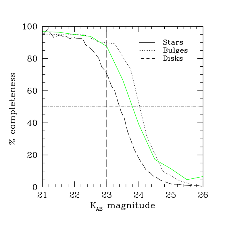
We conducted an extensive set of realistic simulations to determine limiting magnitude as a function of object magnitude and profile. In our simulations, we first created a noiseless image containing a realistic mix of stars, disk-dominated and bulge-dominated galaxies using the TERAPIX software stuff and skymaker. Type-dependent luminosity functions are their evolution with redshift are taken from the VVDS survey (Zucca et al., 2006; Ilbert et al., 2006). The spectral energy distribution (SED) of each galaxy type was modelled using empirical templates of Coleman et al. (1980). The disk size distribution was modelled using the fitting formula and parameters presented in de Jong & Lacey (2000).
Next, we used SExtractor to detect all objects on the stacked image (using the same configuration used to detect objects for the real catalogues) and to produce a CHECKIMAGE in which all these objects were removed (keyword CHECKIMAGE_TYPE -OBJECTS). In the next step this empty background was added to the simulated image, and SExtractor run again in “assoc-mode” in which a match is attempted between each detected galaxy and the output simulated galaxy catalogue produced by stuff. In the last step, the magnitude histograms of the number output galaxies is compared to the magnitude histograms in the input catalogue; this ratio gives the completeness function of each type of object. In total around 30,000 objects (galaxy and stars) in one image were used in these simulations. The results from these simulations are shown in Figure 2. The solid line shows the completeness curve for stars and the dotted line for disks. The completeness fraction is for disks and for stars and bulges at .
In addition to these simulations, we compute upper limits for each filter based on simple noise statistics in apertures of (after applying the noise correction factors listed above). The , limiting magnitude for our data at the centre of the field are , and AB magnitudes for , and magnitudes respectively.
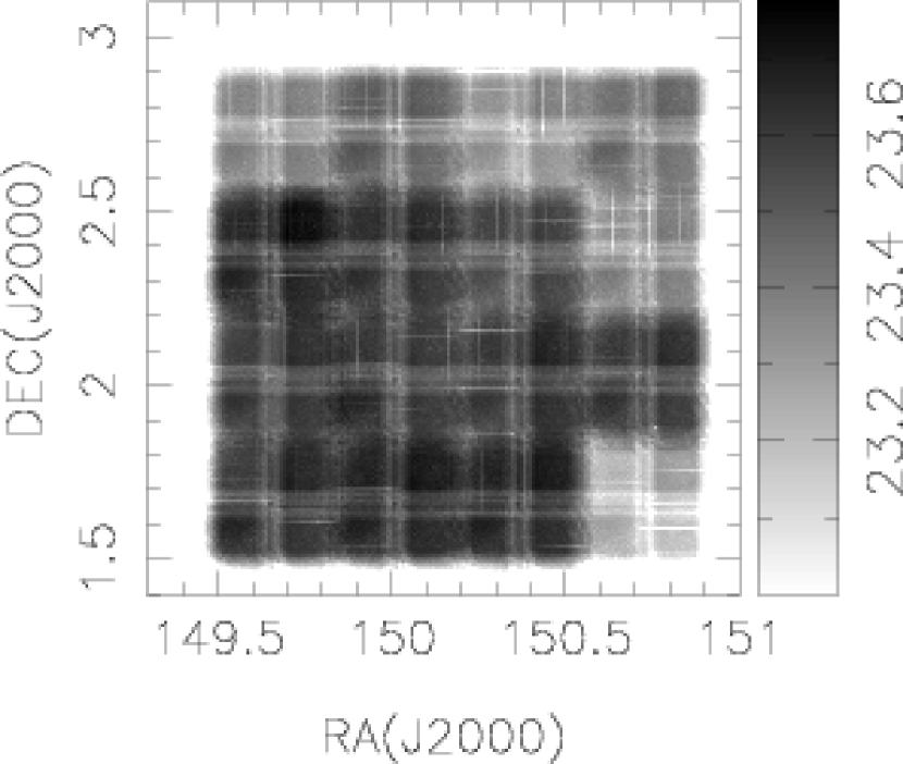
A related issue is the uniformity of the limiting magnitude over the full image. Figure 3 shows the limiting magnitude as a function of position for the stack. This was created by converting the weight map to an rms error map, scaling this error map from per pixel to units of in the effective area of an optimally weighted aperture, and then converting this flux to units of AB magnitude. This depth map agrees well with the completeness limit for point sources shown Figure 2. Note that future COSMOS-WIRCam observations (which will be available in around one years’ time) are expected to further reduce the depth variations across the survey area.
Based on the considerations outlined in this section, we adopt as the limiting magnitude for our catalogues. At this limit our catalogue is greater than and complete for point-sources and galaxies respectively. At this magnitude the number of spurious sources (based on carrying out detections on an image of the stack multiplied by -1) is less than of the total.
3.3. The selection
One of the principal objectives of this paper is to produce a reliable catalogue of objects at using a colour-colour selection technique. A number of different methods now exist to select galaxies in colour-colour space. For instance, the “dropout” technique (Steidel et al., 1996) makes use of Lyman-break spectral feature and the opacity of the high-redshift universe to ultraviolet photons to select star-forming galaxies at , provided they are not too heavily reddened. Similar techniques can be used at (Adelberger et al., 2004; Erb et al., 2003) and large samples of UV-selected star-forming galaxies now exist at these redshifts. At intermediate redshifts, spectroscopy has shown that “ERO” galaxies which are galaxies selected according to red optical-infrared colours contains a mix of old passive galaxies and dusty star-forming systems in the redshift range (Cimatti et al., 2002; Yan et al., 2004). The “DRG” criteria, which selects galaxies with is affected by similar difficulties (Papovich et al., 2006; Kriek et al., 2006). On the other hand, the “” criterion introduced by Daddi et al. (2004) can reliably select galaxies in the redshift range with relatively high completeness and low contamination. Based on the location of star-forming and reddened systems in a spectroscopic control sample lie in the and plane and considerations of galaxy evolutionary tracks, it has been adopted and tested in several subsequent studies (e.g., Kong et al. (2006); Lane et al. (2007); Hayashi et al. (2007); Blanc et al. (2008); Dunne et al. (2009); Popesso et al. (2009)). selected galaxies are estimated to have masses of at (Daddi et al., 2004; Kong et al., 2006).
Compared to other colour criteria, it offers the advantage of distinguishing between actively star-forming and passively-evolving galaxies at intermediate redshifts. It also sharply separates stars from galaxies, and is especially efficient for galaxies. The criterion was originally designed using the redshift evolution in the diagram of various star-forming and passively-evolving template galaxies (i.e., synthetic stellar populations) located over a wide redshift interval. Daddi et al. carried out extensive verifications of their selection criteria using spectroscopic redshifts.
To make the comparison possible with previous studies we wanted our photometric selection criterion to match as closely as possible as the original “BzK” selection proposed in Daddi et al. and adopted by the authors cited above. As our filter set is not the same as this work we applied small offsets (based on the tracks of synthetic stars), following a similar procedure outlined in Kong et al. (2006).
To account for the differences between our Subaru filter and the VLT filter used by Daddi et al. (2004) we use this empirically-derived transformation, defining , then for blue objects with ,
| (6) |
otherwise, for objects with ,
| (7) |
This “” quantity is the actual corrected colour which we use in this paper.
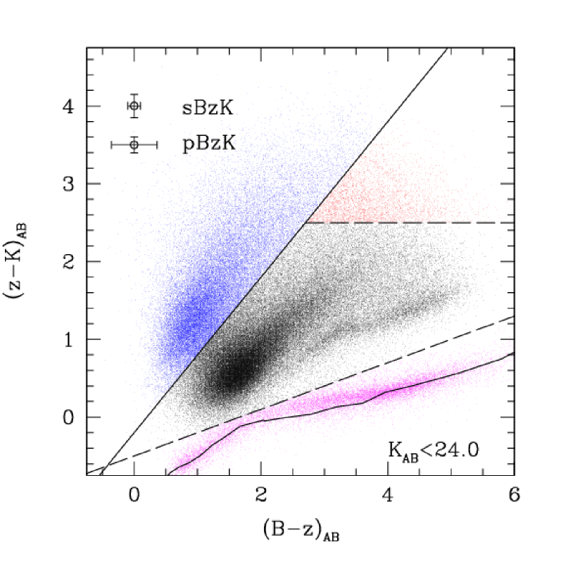
Finally we divide our catalogue into galaxies at , stars, star-forming galaxies and passively evolving galaxies at , by first defining the quantity introduced in Daddi et al. (2004):
| (8) |
For galaxies expected at star-forming galaxies (hereafter ) are selected as those objects with . One should also note that the reddening vector in the plane is approximately parallel to the selection criteria, which ensure that the selection is not biased against heavily reddened dusty galaxies.
Old, passively evolving galaxies (hereafter ) can be selected as those objects which have
| (9) |
Stars are selected using this criteria:
| (10) |
Finally, the full galaxy sample consists simply of objects which do not fulfill this stellarity criterion. The result of this division is illustrated in Figure 4. The solid line represents the colours of stars in the filter set of Daddi et al. using the empirically corrected spectra presented in Lejeune et al. (1997), and it agrees very with our corrected stellar locus.
4. Source counts
We now present number counts of the three populations selected in the previous Section.
4.1. Star and galaxy counts
of Stars, Galaxies and Star-Forming galaxies per Half-magnitude Bin.
| Galaxies | Stars | |||||
|---|---|---|---|---|---|---|
| 16.25 | 102 | 1.73 | ||||
| 16.75 | 204 | 2.03 | ||||
| 17.25 | 487 | 2.41 | ||||
| 17.75 | 838 | 2.65 | ||||
| 18.25 | 1479 | 2.89 | 750 | 2.60 | ||
| 18.75 | 2588 | 3.14 | 928 | 2.69 | ||
| 19.25 | 4073 | 3.33 | 1038 | 2.74 | 24 | 1.10 |
| 19.75 | 6410 | 3.53 | 1138 | 2.78 | 61 | 1.51 |
| 20.25 | 9433 | 3.70 | 1257 | 2.82 | 195 | 2.01 |
| 20.75 | 12987 | 3.84 | 1397 | 2.87 | 710 | 2.57 |
| 21.25 | 17027 | 3.95 | 1425 | 2.88 | 1982 | 3.02 |
| 21.75 | 22453 | 4.07 | 1586 | 2.92 | 4191 | 3.35 |
| 22.25 | 29502 | 4.19 | 1504 | 2.90 | 7684 | 3.61 |
| 22.75 | 36623 | 4.29 | 1596 | 2.93 | 11109 | 3.77 |
Note. — Note. Logarithmic counts are normalised to the effective area of our survey, .
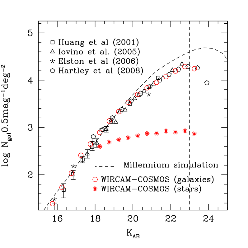
Figure 5 shows our differential galaxy number counts compared to a selection of measurements from the literature. We note that at intermediate magnitudes () counts from the four surveys presented here are remarkably consistent (Elston et al., 2006; Huang et al., 1997; Hartley et al., 2008). At discrepancies between different groups concerning measurement of total magnitudes and star-galaxy separation leads to an increased scatter. At these magnitudes, shot noise and large-scale-structure begin to dominate the number count errors.
The COSMOS-WIRCam survey is currently the only work to provide unbroken coverage over the range . In addition, our colour-selected star-galaxy separation provides a very robust way to reject stars from our faint galaxy sample. These stellar counts are shown by the asterisks in Figure 5. We note that at magnitudes brighter than our stellar number counts become incomplete because of saturation in the Subaru image (our catalogues exclude any objects with saturated pixels which preferentially affect point-like sources). Our galaxy and star number counts are reported in Table 2.
4.2. and counts
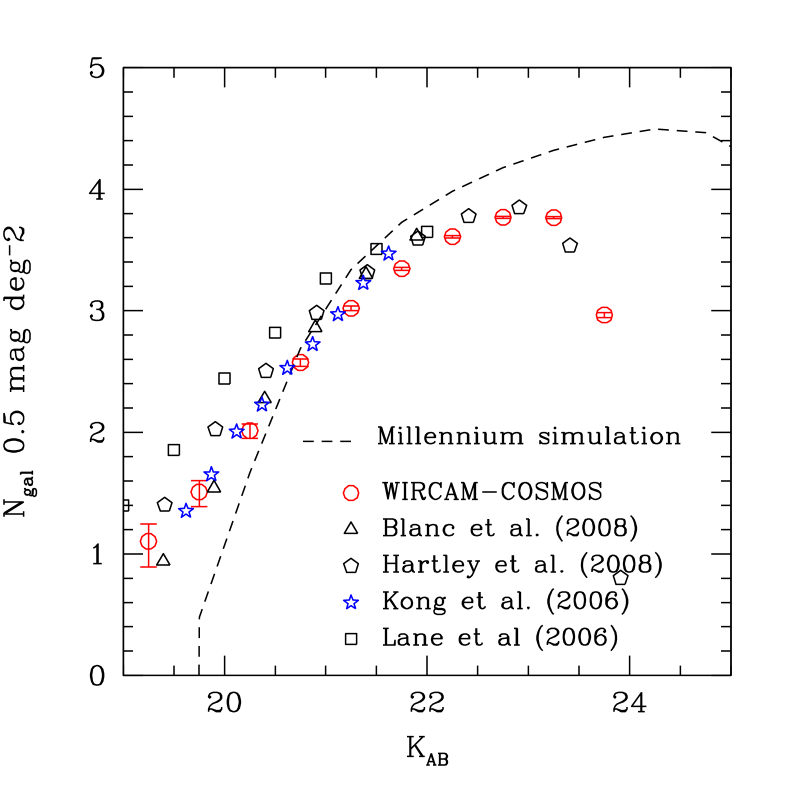
Figure 6 shows the counts of star-forming galaxies compared to measurements from the literature. These counts are summarised in Table 2. We note an excellent agreement with the counts in Kong et al. (2006) and the counts presented by the MUYSC collaboration (Blanc et al., 2008). However, the counts presented by the UKIDSS-UDS group (Lane et al., 2007; Hartley et al., 2008) are significantly offset compared to our counts at bright magnitudes, and become consistent with it by . These authors attribute the discrepancy to cosmic variance but we find photometric offsets a more likely explanation (see below).
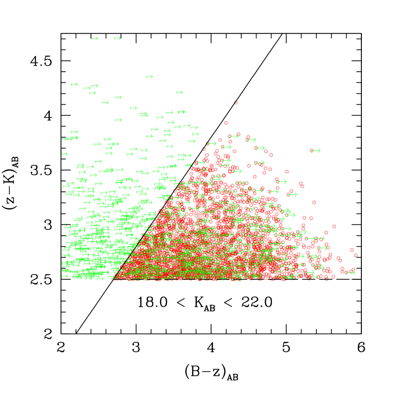
Figure 7 shows in more detail the zone occupied by passive galaxies in Figure 4. Left of the diagonal line are objects classified as star-forming galaxies. Objects not detected in are plotted as right-pointing arrows with colours computed from the upper limit of their magnitudes. An object is considered undetected if the flux in a 2″aperture is less than the corrected noise limit. For the band this corresponds to approximately 29.1 mag. This criterion means that in addition to the galaxies already in the selection box, fainter with -band non-detections (shown with the green arrows) may be scattered rightward into the region.
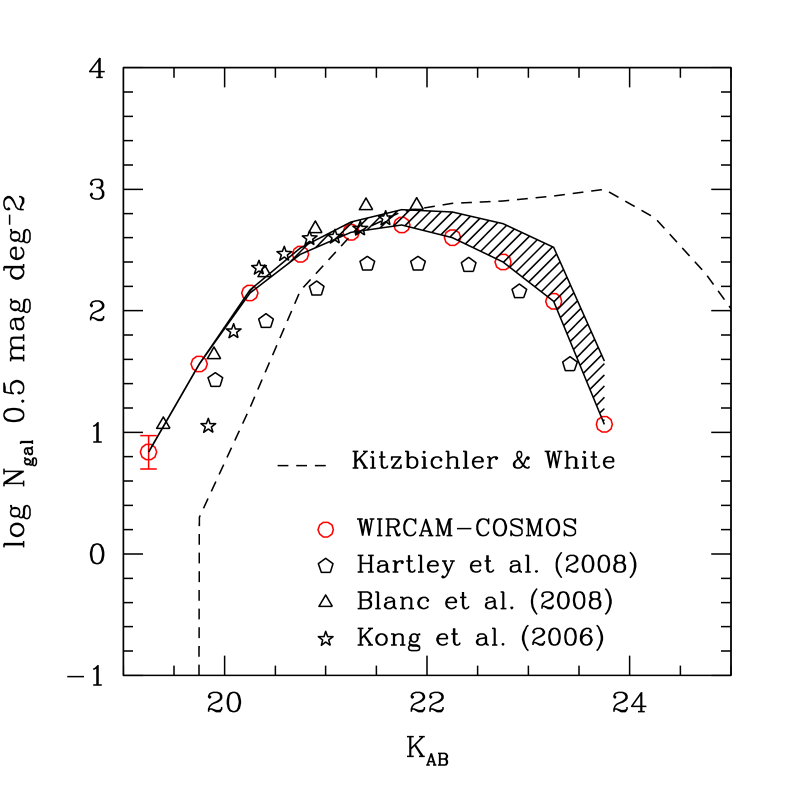
Counts for our passive galaxy population including these “additional” objects are represented by the hatched region in Figure 8. The upper limit for the source counts in this figure represents the case in which all the sources undetected in are scattered into the region. Even accounting for these additional objects we unambiguously observe a flattening and subsequent turnover in the passive galaxy counts at around , well above the completeness limit of either our or data in agreement with (Hartley et al., 2008).
This upper limit, however, is a conservative estimate. We have made a better estimate of this upper limit by carrying out a stacking analysis of the objects not detected in in both the passive and star-forming regions of the diagram. For each apparent magnitude bin in Table we median-combine Subaru band postage stamps for objects with no -band detection, producing separate stacks for the star-forming and passive regions of the diagram. In both cases, objects below our detection limit are clearly visible (better than a three-sigma detection) in our stacked images at each magnitude bin to . By assuming that the mean magnitude of the stacked source to be the average magnitude of our undetected sources, we can compute the average colour of our undetected sources, and reassign their location in the diagram if necessary. This experiment shows that at most only of the star-forming galaxies undetected in move to the passive region.
Our number counts are summarised in Table 3, which also indicates the upper count limits based on band observations. As before, our counts are in good agreement with those presented in Kong et al. (2006) and Blanc et al. (2008) but are above the counts in Hartley et al. (2008).
To investigate the origin of this discrepancy, we compared our diagram with Hartley et al.’s, which should also be in the Daddi et al. filter set. We superposed our diagram on that of Hartley et al. and found that the Hartley et al. stellar locus is bluer by in both and compared to our measurements666Since the first draft of this manuscript was prepared, a communication with W. Hartley has confirmed that the transformations to the Daddi et al. system were incorrectly computed in their work.. We have already seen that our stellar locus agrees well with the theoretical stellar sequence computed using the Lejeune et al. (1997) synthetic spectra in the Daddi et al. filter set and also with the stellar locus presented in Daddi et al. and Kong et al.. We conclude therefore that the number counts discrepancies arise from an incorrect transformation to the Daddi et al. filter set.
| Passive | Passive (upper limits)aaThe upper limit to the was computed by including all the galaxies undetected in with | |||
|---|---|---|---|---|
| 19.25 | 13 | 0.84 | 13 | 0.84 |
| 19.75 | 69 | 1.56 | 69 | 1.56 |
| 20.25 | 265 | 2.15 | 280 | 2.17 |
| 20.75 | 553 | 2.47 | 621 | 2.52 |
| 21.25 | 837 | 2.65 | 1015 | 2.73 |
| 21.75 | 963 | 2.71 | 1285 | 2.83 |
| 22.25 | 757 | 2.60 | 1229 | 2.81 |
| 22.75 | 475 | 2.40 | 984 | 2.72 |
Note. — Logarithmic counts are normalised to the effective area of our survey, .
4.3. Comparison with the Semi-analytic Model of Kitzbichler & White
In Figures 5, 6 and 8 we show counts of galaxies extracted from the semi-analytical model presented in Kitzbichler & White (2007).
Semi-analytic models start from either an analytic “merger tree” of dark matter haloes or, in the case of the model used here, merger trees derived from a numerical simulation, the Millennium simulation (Springel et al., 2005)). Galaxies are “painted” onto dark matter haloes using a variety of analytical recipes which include treatments of gas cooling, star-formation, supernovae feedback, and black hole growth by accretion and merging. An important recent advance has been the addition of “radio mode” AGN feedback Bower et al. (2006); Croton et al. (2007) which helps provide a better fit to observed galaxy luminosity functions. The Kitzbichler & White model is derived from the work presented by Croton et al. (2006) and further refined by Lucia & Blaizot (2007). It differs only from these papers in the inclusion of a refined dust model. We refer the readers to these works for further details. An extensive review of semi-analytic modelling techniques can be found in Baugh (2006).
To derive counts of quiescent galaxies, we follow the approach of Daddi et al. (2007) and select all galaxies at in the star-formation rate - mass plane (Figure 18 from Daddi et al.) which have star-formation rates less than three times the median value for a given mass. Star-forming objects were defined as those galaxies which do not obey this criterion, in this redshift range. (Unfortunately the publicly available data do not contain all the COSMOS bands so we cannot directly apply the selection criterion to them.).
In all three plots, the models over-predict the number of faint galaxies, an effect already observed for the selected samples investigated in Kitzbichler & White. We also note that adding an upper redshift cut to the model catalogues to match our photometric redshift distributions (see later) does not change appreciably the number of predicted galaxies.
Considering in more detail the counts of quiescent galaxies we find that at models are below observations by a factor of two, whereas at model counts are in excess of observations by around a factor of 1.5. Given the narrow redshift range of our passive galaxy population, apparent magnitude is a good proxy for absolute magnitude which can itself be directly related to underlying stellar mass Daddi et al. (2004). This implies that these models predict too many small, low-mass passively-evolving galaxies and too few large high mass passively evolving galaxies at .
It is instructive to compare our results with Figure 7 from Kitzbichler & White, which shows the stellar mass function for their models. At , the models both under-predict the number of massive objects and over-predict the number of less massive objects, an effect mirroring the overabundance of luminous objects with respect to the Kitzbichler & White model seen in our data.
A similar conclusion was drawn by Fontana et al. (2006) who recently compared predictions for the galaxy stellar mass function for massive galaxies for a variety of models with observations of massive galaxies up to in the GOODS field. They also concluded that models incorporating AGN feedback similar to Kitzbichler & White under-predicted the number of high mass galaxies.
Thanks to the wide-area, deep band data available in the COSMOS field, we are able to make reliable measurements of the number of faint passive galaxies. Reassuringly, the turnover in counts of passive galaxies observed in our data is qualitatively in agreement with the measurements of the faint end of the mass function of quiescent galaxies at made in Ilbert et al. (2009b).
5. Photometric redshifts for the and population
For many years studies of galaxy clustering at have been hindered by our imperfect knowledge of the source redshift distribution and small survey fields. Coverage of the COSMOS field in thirty broad, intermediate and narrow photometric bands has enabled the computation of very precise photometric redshifts (Ilbert et al., 2009a).
These photometric redshifts were computed using deep Subaru data described in Capak et al. (2007) combined with intermediate band data, the data presented in this paper, data from near-infrared camera WFCAM at the United Kingdom Infrared Telescope and IRAC data from the Spitzer-COSMOS survey (sCOSMOS, Sanders et al. (2007)). These near- and mid-infrared bandpasses are an essential ingredient to compute accurate photometric redshifts in the redshift range , in particular because they permit the location of the Å break to be determined accurately. Moreover, spectroscopic redshifts of 148 galaxies with a from the early zCOSMOS survey (Lilly et al., 2007b) have been used to check and train these photometric redshifts in this important redshift range.
A set of templates generated by Polletta et al. (2007) using the GRASIL code Silva et al. (1998) are used . The nine galaxy templates of Polletta et al. include three SEDs of elliptical galaxies and six spiral galaxies templates (S0, Sa, Sb, Sc, Sd, Sdm). This library is complemented with 12 additional blue templates generated using the models ofBruzual & Charlot (2003).
The photometric redshifts are computed using a standard template fitting procedure (using the “Le Phare” code). Biases in the photo-z are removed by iterative calibration of the photometric band zero-points. This calibration is based on 4148 spectroscopic redshifts at from the zCOSMOS survey Lilly et al. (2007b). As suggested by the data, two different dust extinction laws Prevot et al. (1984); Calzetti et al. (2000) were applied specific to the different SED templates. A new method to account for emission lines was implemented using relations between the UV continuum and the emission line fluxes associated with star formation activity.
Based on a comparison between photometric redshifts and 4148 spectroscopic redshifts from zCOSMOS, we estimate an accuracy of for the galaxies brighter than . We extrapolate this result at fainter magnitude based on the analysis of the 1 errors on the photo-z. At , we estimate an accuracy of , at , , respectively.
5.1. Photometric redshift distributions

We have cross-correlated our catalogue with photometric redshifts to derive redshift selection functions for each photometrically-defined galaxy population. Note that although photometric redshifts are based on an optically-selected catalogue, this catalogue is very deep () and contains almost all the objects present in the -band selected catalogue. At , 138376 were successfully assigned photometric redshifts, representing of the total galaxy population.
Figure 9 shows the redshift distribution for all -selected galaxies, as well as for -selected passively-evolving and star-forming galaxies in the magnitude range . We have computed the redshift selection function in several magnitude bins and found that the effective redshift does not depend significantly on apparent magnitude for the and populations.
By using only the blue grism of the VIMOS spectrograph at the VLT, the zCOSMOS-Deep survey is not designed to target galaxies, and so no spectroscopic redshifts were available to train the photometric redshifts of objects over the COSMOS field. At these redshifts the main spectral features of galaxies, namely Ca II H& K and the 4000 Å break, have moved to the near infrared. Hence, optical spectroscopy can only deliver redshifts based on identifying the so called Mg-UV feature at around 2800Å in the rest frame. All in all, spectroscopic redshifts of passive galaxies at are now available for only a few dozen objects (Glazebrook et al., 2004; Daddi et al., 2005; Kriek et al., 2006; McGrath et al., 2007; Cimatti et al., 2008). We note that the average spectroscopic redshift of these objects () indicates that the average photometric redshift of of our galaxies to the same -band limit may be systematically underestimated. For the medium to short term one has to unavoidably photometric redshifts when redshifts are needed for large numbers of passive galaxies at .

From Figure 9 we can estimate the relative contribution of each classification type to the total number of galaxies to at least . This is shown in Figure 10, where we show for each bin in photometric redshift the number of each selection class as a fraction of the total number of galaxies. Upper and lower confidence limits are computed using Poisson statistics and the small-number approximation of Gehrels (1986); in general we can make reliable measurements to . In the redshift range at the population represents around of the total number of galaxies, in contrast to for -selected galaxies. The sum of both components represents at most of the total population at .
We estimate the fraction of DRG galaxies using band data described in Capak et al. (2007). DRG-selected galaxies remain an important fraction of the total galaxy population, reaching around of the total at . This in contrast with Reddy et al. (2005) who found no significant overlap in the spectroscopic redshift distributions of and DRG galaxies.
Our work confirms that most bright passive- galaxies lie in a narrower redshift range than either the or the DRG selection. We also see that the distribution in photometric redshifts for the DRG galaxies is quite broad. Similar conclusions were reached by Grazian et al. (2007) and Daddi et al. (2004) using a much smaller, fainter sample of galaxies.
6. Clustering properties
6.1. Methods
For each object class we measure , the angular correlation function, using the standard Landy & Szalay (1993) estimator:
| (11) |
where , and are the number of data–data, data–random and random–random pairs with separations between and . These pair counts are appropriately normalised; we typically generate random catalogues with ten times higher numbers of random points than input galaxies. We compute at a range of angular separations in logarithmically spaced bins from to with , where is in degrees. At each angular bin we use bootstrap errors to estimate the errors in . Although these are not in general a perfect substitute for a full estimate of cosmic variance (e.g. using an ensemble of numerical simulations), they should give the correct magnitude of the uncertainty (Mo et al., 1992).
We use a sorted linked list estimator to minimise the computation time required. The fitted amplitudes quoted in this paper assume a power-law slope for the galaxy correlation function, ; however this amplitude must be adjusted for the ‘integral constraint’ correction, arising from the need to estimate the mean galaxy density from the sample itself. This can be estimated as (e.g. Adelberger et al., 2005),
| (12) |
Our quoted fitted amplitudes are are corrected for this integral constraint, i.e., we fit
| (13) |
For the COSMOS field, for . An added complication is that the integral constraint correction depends weakly on the slope,; in fitting simultaneously and we use an interpolated look-up table of values for in our minimisation procedure.
Finally, it should be mentioned that in recent years it has become increasingly clear that the power-law approximation for is no longer appropriate (see for example, Zehavi et al. (2004)). In reality, the observed is the sum of the contributions of galaxy pairs in separate dark matter haloes and within the same halo of dark matter; it is only in a few fortuitous circumstances that this observed is well approximated by a power law of slope . We defer a detailed investigation of the shape of in terms of these “halo occupation models” to a second paper, but these points should be borne in mind in the forthcoming analysis.
6.2. Clustering of galaxies and stars
To verify the stability and homogeneity of our photometric calibration over the full of the COSMOS field we first compute the correlation function for stellar sources. These stars, primarily residing in the galactic halo, should be unclustered. They are identified as objects below the diagonal line in Figure 4. This classification technique is more robust than the usual size or compactness criterion, which can include unresolved galaxies.

The amplitude of as a function of angular scale for stars and faint galaxies is shown in Figure 11. For comparison we have also plotted the clustering amplitude for our faintest selected galaxy sample. The inset plot shows a zoom on measurements at large scale scales where the amplitude of is very low. At each angular bin our stellar correlation function is consistent with zero out to degree scales down to a limiting magnitude of . If we fit a power-law correlation function of slope 0.8 to our stellar clustering measurements we find (at ; in comparison, the faintest galaxy correlation function signal we measure is , around times larger.
Figure 12 shows for galaxies in three magnitude slices. It is clear that the slope of becomes shallower at fainter magnitudes. At small separations (less than ) decreases due to object blending. Our fitted correlation amplitudes and slopes for field galaxies are reported in Table 4.
| 18.5 | ||
| 19.0 | ||
| 19.5 | ||
| 20.0 | ||
| 20.5 | ||
| 21.0 | ||
| 21.5 | ||
| 22.0 | ||
| 22.5 | ||
| 23.0 |


In Figure 13 we investigate further the dependence of slope on limiting magnitude. Here we fit for the slope and amplitude simultaneously for all slices. At bright magnitudes the slope corresponds to the canonical value of ; towards intermediate magnitudes it becomes steeper and fainter magnitudes progressively flatter. It is interesting to compare this Figure with the COSMOS optical correlation function presented in Figure 3 of McCracken et al. (2007) which also showed that the slope of the angular correlation function becomes progressively shallower at fainter magnitudes. One possible interpretation of this behaviour is that at bright magnitudes our -selected samples are dominated by bright, red galaxies which have an intrinsically steeper correlation function slope; our fainter samples are predominantly bluer, intrinsically fainter objects with shallower intrinsic correlation function slope.
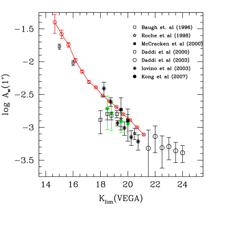
Finally, it is instructive to compare our field galaxy clustering amplitudes with literature measurements as our survey is by far the largest at these magnitude limits. Figure 14 shows the scaling of the correlation amplitude at one degree as a function to limiting magnitude, compared a compilation of measurements from the literature. To make this comparison, we have assumed a fixed slope of and converted the limiting magnitude of each of our catalogues to Vega magnitudes.
In general our results are within the error bars of most measurements, although it does appear that the COSMOS field is slightly more clustered than other fields in the literature, as we have discussed previously (McCracken et al., 2007).
6.3. Galaxy clustering at
In the previous Sections we have demonstrated the reliability of our estimates of and our general agreement with preceding literature measurements for magnitude-limited samples. We now investigate the clustering properties of passive and star-forming galaxy candidates at selected using our diagram. Figure 15 shows the spatial distribution of the galaxies in our sample; a large amount of small-scale clustering is evident.

| Passive | Star-forming | |||
|---|---|---|---|---|
| 22.0 | ||||
| 23.0 | ||||
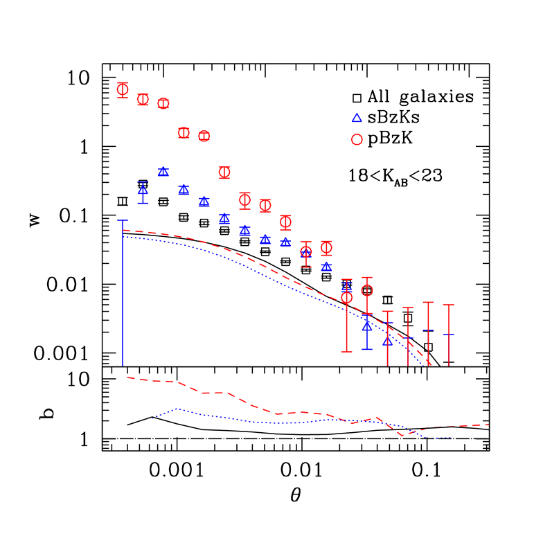
The upper panel of Figure 16 shows the angular correlation functions for our , and for all galaxies. In each case we apply a magnitude cut. For comparison we show the clustering amplitude of dark matter computed using the redshift selection functions presented in Section 5 and the non-linear power spectrum approximation given in Smith et al. (2003). At intermediate to large scales, the clustering amplitude of field galaxies and the population follows very well the underlying dark matter.
The lower panel of Figure 16 shows the bias , as a function of scale, computed simply as . Dashed, dotted and solid lines show values for , and field galaxies retrospectively (in this case our measurements have been corrected for the integral constraint). The bias for the faint field galaxy population is 1.2 at indicating that the faint selected galaxy population traces well the underlying dark matter. In comparison, at the same scales, the bias values for the passive and star-forming galaxies are 2.5 and 2.1 respectively.
Our best-fitting and amplitudes (quoted at ) for and galaxies are reported in Table 5. Given that for the galaxies we may compare with previous authors who generally assume a fixed slope for all measurements. At , corresponding to , Kong et al. (2006) find whereas (at ) we measure , closer to the value of found by Blanc et al. (2008). We note that both Hayashi et al. (2007) and Adelberger et al. (2005) also investigated the luminosity dependence of galaxy clustering at although with samples considerable smaller than those presented here. It is plausible that field-to-field variation and large scale structure are the cause of the discrepancy between these surveys.
The best fitting slopes for our populations is , considerably steeper than the field galaxy population (no previous works have attempted to fit both slope and amplitude simultaneously for the populations due to small sample sizes). In the next section we will derive the spatial clustering properties of both populations.
6.4. Spatial clustering
To de-project our measured clustering amplitudes and calculate the comoving correlation lengths at the effective redshifts of our survey slices we use the photometric redshift distributions presented in Section 5.
Given a redshift interval and a redshift distribution we define the effective redshift in the usual way, namely, is defined as
| (14) |
Using these redshift distributions together with the fitted correlation amplitudes in presented in Sections 6.2 and 6.3 we can derive the comoving correlation lengths of each galaxy population at their effective redshifts using the usual Limber (1953); Peebles (1980) inversion. We assume that does not change over the redshift interval probed.
It is clear that our use of photometric redshifts introduces an additional uncertainty in . We attempted to estimate this uncertainty by using the probability distribution functions associated with each photometric redshift to compute an ensemble of values, each estimated with a different . The resulting error in from these many realisations is actually quite small, for the population. Of course, systematic errors in the photometric redshifts could well be much higher than this. Figure 9. in Ilbert et al. shows the error in the photometric redshifts as a function of magnitude and redshift. Although all galaxy types are combined here, we can see that the approximate error in the photometric redshifts between is . Our estimate of the correlation length is primarily sensitive to the median redshift and the width of the correlation length. An error translates into an error of in . We conclude that, for our and measurements, the dominant source of uncertainty in our measurements of comes from our errors on .
We note that previous investigations of the correlation of passive galaxies always assumed a fixed ; from Figure 12 it is clear that our slope is much steeper. These surveys, however, fitted over a smaller range of angular scales and therefore could not make an accurate determination of the slope for the population. In all cases we fit for both and .
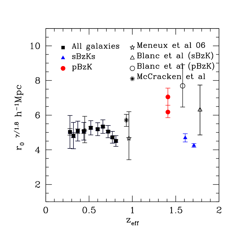
Our spatial correlation amplitudes for and galaxies are summarised in Table 6. Because of the degeneracy between and we also quote clustering measurements as . These measurements are plotted in Figure 17. At lower redshifts, our field galaxy samples are in good agreement with measurements for optically selected redder galaxies from the CFHTLS and VVDS surveys (Meneux et al., 2006; McCracken et al., 2008). At higher redshifts, our clustering measurements for and galaxies are in approximate agreement with the measurements of Blanc et al. (2008). We note that part of the differences with the measurements of Blanc et al. arises from the their approximation of the redshift distribution of passive galaxies using simple Gaussian distribution.
Interestingly, a steep slope for optically-selected passive galaxies has already been reported at lower redshift surveys; for example, Madgwick et al. (2003) found that passive galaxies had a much steeper slope than active galaxies in the 2dF galaxy redshift survey.
The highly biased nature of the galaxy population indicates that these objects reside in more massive dark matter haloes than either the field galaxy population or the population, and we intend to present a more detailed discussion of the spatial clustering of each galaxy sample in the framework of the halo occupation models in a future paper.
| Passive galaxies | Star-forming galaxies | |||||
|---|---|---|---|---|---|---|
| 22.0 | 1.41 | 1.61 | ||||
| 23.0 | 1.41 | 1.71 | ||||
7. Summary and conclusions
We have presented counts, colours and clustering properties for a large sample of selected galaxies in the COSMOS-WIRCam survey. This represents the largest sample of galaxies to date at this magnitude limit. By adding deep Subaru and data we are able to classify our catalogue into star-forming and quiescent/passive objects using the selection criterion proposed by Daddi et al. (2004). To our catalogues comprises galaxies, of which are classified as passive galaxies and as star-forming galaxies. We have also identified a large sample of faint stars.
Counts of field galaxies and star-forming galaxies change slope at . Our number counts of quiescent galaxies turns over at , confirming an observation previously made in shallower surveys (Lane et al., 2007). This effect cannot be explained by incompleteness in any of our very deep optical bands. Our number counts of passive, star-forming and field galaxies agree well with surveys with brighter magnitude limits.
We have compared our counts to objects selected in a semi-analytic model of galaxy formation. For simple magnitude-limited samples the Kitzbichler & White (2007) model reproduces very well galaxy counts in the range . However, at fainter magnitudes Kitzbichler & White’s model predict many more objects than are observed.
Comparing this model with predictions of passive galaxy counts, we find that at model counts are below observations by a factor of 2, whereas at model counts are in excess of observations by around a factor of 1.5. This implies that the Kitzbichler & White model predicts too many small, low-mass passively-evolving galaxies and too few large high-mass passively evolving galaxies at . In these models, bulge formation takes place by mergers. At , passive galaxies in the millennium simulation have stellar masses of , similar to spectroscopic measurements of passive galaxies (Kriek et al., 2006). This suggests that the difference between models and observations is linked to the amount of “late merging” taking place (Lucia & Blaizot, 2007). The exact choice of the AGN feedback model can also sensitively affect the amount star-formation in massive systems (Lucia et al., 2006; Bower et al., 2006). It is clear that observations of the abundance of massive galaxies can now provide insight into physical processes occurring in galaxies at intermediate redshifts. For the time being it remains a challenge for these models to reproduce both these observations at high redshift and lower-redshift reference samples.
Our results complement determinations of the galaxy stellar mass function at intermediate redshifts which show that total mass in stars formed in semi-analytic models is too low at compared to models (Fontana et al., 2006). We note that convolution with standard uncertainties of dex in mass function estimates at can make a significant difference in the mass function, as can be see in Figure 14 of Wang et al. (2008) who show detailed comparisons between semi-analytic models and observations. The discrepancy between our observations and models cannot be explained in this way.
We have cross-matched our catalogue with precise 30-band photometric redshifts calculated by Ilbert et al. and have used this to derive the redshift distributions for each galaxy population. At our passive galaxies have a redshift distribution with , in approximate agreement with similar spectroscopic surveys comprising smaller numbers of objects. Most of our galaxies have , in contrast with the redshift distribution for galaxies and for the general field galaxy population which extend to much higher redshifts at this magnitude limit. In the redshift range at the population represents around of the total number of galaxies, in contrast to for -selected galaxies. DRG-selected galaxies remain an important fraction of the total galaxy population, reaching around of the total at . Our work confirms that most galaxies satisfying the passive- selection criteria lie in a narrower redshift than either - or DRG-selected objects. Interestingly, a few a passive galaxies in our survey have , and it is tempting to associate these objects with higher-redshift evolved galaxies detected in spectroscopic surveys (Kriek et al., 2008). We have investigated the clustering properties of our catalogues for which the field of view of the COSMOS survey provides a unique probe of the distant universe. Our stellar correlation function is zero at all angular scales to demonstrating the photometric homogeneity and stability of our catalogues. For a selected samples, the clustering amplitude declines monotonically toward fainter magnitudes. However, the slope of the best-fitting angular correlation function becomes progressively shallower at fainter magnitudes, an effect already seen in the COSMOS optical catalogues.
At the faintest magnitude slices, the field galaxy population (all objects with ) is only slightly more clustered than the underlying dark matter distribution, indicating that selected samples are excellent tracers of the underlying mass. On the other hand, star-forming and passive galaxy candidates are more clustered than the field galaxy population. At arcminute scales and smaller the passive BzK population is strongly biased with respect to the dark matter distribution with bias values of 2.5 and higher, depending on scale.
Using our photometric redshift distributions, we have derived the comoving correlation length for each galaxy class. Fitting simultaneously for slope and amplitude we find a comoving correlation length of Mpc for the passive population and Mpc for the star-forming galaxies at . Our field galaxy clustering amplitudes are in approximate agreement with optically-selected red galaxies at lower redshifts.
High bias values are consistent with a picture in which galaxies inhabit relatively massive dark matter haloes on order of M⊙, compared to the and field galaxy population. We will return to this point in future papers, where will interpret these measurements in terms of the halo model.
Measuring spectroscopic redshifts for a major fraction of 3000 galaxies in the COSMOS field one will have to wait for the advent of large-throughput, wide-field near-infrared (-band) spectrographs on 8-10m class telescopes, such as FMOS at Subaru (Kimura et al. 2006). Smaller field, cryogenic, multi-object spectrographs such as MOIRCS at Subaru (Ichikawa et al., 2006), EMIR at the GTC telescope (Garzón et al., 2006), and Lucifer at the LBT (Mandel et al., 2006) should prove effective in producing high S/N spectra for a relatively small fraction of the galaxies in the COSMOS field.
Since this paper was prepared, additional COSMOS-WIRCam data observations have been taken which will increase the total exposure time by . In addition, new - observations have also been made. Both these data products will be made publicly available in around one year from the publication of this article. In the longer term, the COSMOS field will be observed as part of the UltraVISTA deep near-infrared survey which will provide extremely deep observations over the central part of the field.
8. Acknowledgements
This work is based in part on data products produced at TERAPIX at the Institut d’Astrophysique de Paris. H.J. McC acknowledges the use of TERAPIX computing facilities and the hospitality of the IfA, Honolulu, where this paper was finished. M. L. Kilbinger is acknowledged for help with dark matter models in Section 6 and N. V. Asari for the stacking analysis in Section 4. This research has made use of the VizieR catalogue access tool provided by the CDS, Strasbourg, France. This research was supported by ANR grant “ANR-07-BLAN-0228”. ED and CM also acknowledge support from “ANR-08-JCJC-0008”. JPK acknowledges support from the CNRS. We thank the referee for an extensive commentary on a earlier version of this paper.
References
- Abraham et al. (2004) Abraham, R. G., et al. 2004, AJ, 127, 2455
- Adelberger et al. (2005) Adelberger, K. L., Steidel, C. C., Pettini, M., Shapley, A. E., Reddy, N. A., & Erb, D. K. 2005, ApJ, 619, 697
- Adelberger et al. (2004) Adelberger, K. L., Steidel, C. C., Shapley, A. E., Hunt, M. P., Erb, D. K., Reddy, N. A., & Pettini, M. 2004, ApJ, 607, 226
- Arnouts et al. (2007) Arnouts, S., et al. 2007, A&A, 476, 137
- Baugh (2006) Baugh, C. M. 2006, Reports on Progress in Physics, 69, 3101
- Baugh et al. (1996) Baugh, C. M., Gardner, J. P., Frenk, C. S., & Sharples, R. M. 1996, MNRAS, 283, L15
- Bell et al. (2004) Bell, E. F., et al. 2004, ApJ, 608, 752
- Bertin (2006) Bertin, E. 2006, in Astronomical Society of the Pacific Conference Series, Vol. 351, Astronomical Data Analysis Software and Systems XV, ed. C. Gabriel, C. Arviset, D. Ponz, & S. Enrique, 112–+
- Bertin & Arnouts (1996) Bertin, E., & Arnouts, S. 1996, A&A, 117, 393
- Bertin et al. (2002) Bertin, E., Mellier, Y., Radovich, M., Missonnier, G., Didelon, P., & Morin, B. 2002, Astronomical Data Analysis Software and Systems XI, 281, 228
- Blanc et al. (2008) Blanc, G. A., et al. 2008, ApJ, 681, 1099
- Bower et al. (2006) Bower, R. G., Benson, A. J., Malbon, R., Helly, J. C., Frenk, C. S., Baugh, C. M., Cole, S., & Lacey, C. G. 2006, MNRAS, 370, 645
- Bruzual & Charlot (2003) Bruzual, G., & Charlot, S. 2003, MNRAS, 344, 1000
- Calzetti et al. (2000) Calzetti, D., Armus, L., Bohlin, R. C., Kinney, A. L., Koornneef, J., & Storchi-Bergmann, T. 2000, ApJ, 533, 682
- Capak et al. (2007) Capak, P., et al. 2007, ApJS, 172, 99
- Cimatti et al. (2002) Cimatti, A., et al. 2002, A&A, 381, L68
- Cimatti et al. (2008) —. 2008, A&A, 482, 21
- Coleman et al. (1980) Coleman, G. D., Wu, C.-C., & Weedman, D. W. 1980, ApJS, 43, 393
- Connolly et al. (1997) Connolly, A. J., Szalay, A. S., Dickinson, M., Subbarao, M. U., & Brunner, R. J. 1997, ApJ, 486, L11
- Conroy et al. (2009) Conroy, C., Gunn, J. E., & White, M. 2009, ApJ, 699, 486
- Cowie et al. (1994) Cowie, L. L., Gardner, J. P., Hu, E. M., Songaila, A., Hodapp, K.-W., & Wainscoat, R. J. 1994, ApJ, 434, 114
- Cowie et al. (1996) Cowie, L. L., Songaila, A., Hu, E. M., & Cohen, J. G. 1996, AJ, 112, 839
- Croton et al. (2007) Croton, D. J., Gao, L., & White, S. D. M. 2007, MNRAS, 374, 1303
- Croton et al. (2006) Croton, D. J., et al. 2006, MNRAS, 365, 11
- Daddi et al. (2000) Daddi, E., Cimatti, A., Pozzetti, L., Hoekstra, H., Röttgering, H. J. A., Renzini, A., Zamorani, G., & Mannucci, F. 2000, A&A, 361, 535
- Daddi et al. (2004) Daddi, E., Cimatti, A., Renzini, A., Fontana, A., Mignoli, M., Pozzetti, L., Tozzi, P., & Zamorani, G. 2004, ApJ, 617, 746
- Daddi et al. (2005) Daddi, E., et al. 2005, ApJ, 631, L13
- Daddi et al. (2007) —. 2007, ApJ, 670, 156
- de Jong & Lacey (2000) de Jong, R. S., & Lacey, C. 2000, ApJ, 545, 781
- Dickinson et al. (2003) Dickinson, M., Papovich, C., Ferguson, H. C., & Budavári, T. 2003, ApJ, 587, 25
- Drory et al. (2005) Drory, N., Salvato, M., Gabasch, A., Bender, R., Hopp, U., Feulner, G., & Pannella, M. 2005, ApJ, 619, L131
- Dunne et al. (2009) Dunne, L., et al. 2009, MNRAS, 394, 3
- Elston et al. (2006) Elston, R. J., et al. 2006, ApJ, 639, 816
- Erb et al. (2003) Erb, D. K., Shapley, A. E., Steidel, C. C., Pettini, M., Adelberger, K. L., Hunt, M. P., Moorwood, A. F. M., & Cuby, J.-G. 2003, ApJ, 591, 101
- Faber et al. (2007) Faber, S. M., et al. 2007, ApJ, 665, 265
- Fèvre et al. (2005) Fèvre, O. L., et al. 2005, Nature, 437, 519
- Fontana et al. (2004) Fontana, A., et al. 2004, A&A, 424, 23
- Fontana et al. (2006) —. 2006, A&A, 459, 745
- Franx et al. (2003) Franx, M., et al. 2003, ApJ, 587, L79
- Garzón et al. (2006) Garzón, F., et al. 2006, Proc. SPIE, 6269, 40
- Gehrels (1986) Gehrels, N. 1986, ApJ, 303, 336
- Glazebrook et al. (2004) Glazebrook, K., et al. 2004, Nature, 430, 181
- Grazian et al. (2007) Grazian, A., et al. 2007, A&A, 465, 393
- Hartley et al. (2008) Hartley, W. G., et al. 2008, MNRAS, 391, 1301
- Hayashi et al. (2007) Hayashi, M., Shimasaku, K., Motohara, K., Yoshida, M., Okamura, S., & Kashikawa, N. 2007, ApJ, 660, 72
- Hu & Ridgway (1994) Hu, E. M., & Ridgway, S. E. 1994, AJ, 107, 1303
- Huang et al. (1997) Huang, J., Cowie, L. L., Gardner, J. P., Hu, E. M., Songaila, A., & Wainscoat, R. J. 1997, ApJ, 476, 12+
- Ichikawa et al. (2006) Ichikawa, T., et al. 2006, Proc. SPIE, 6269, 38
- Ilbert et al. (2005) Ilbert, O., et al. 2005, A&A, 439, 863
- Ilbert et al. (2006) Ilbert, O., et al. 2006, A&A, 453, 809
- Ilbert et al. (2009a) —. 2009a, ApJ, 690, 1236
- Ilbert et al. (2009b) —. 2009b, ArXiv:0903.0102
- Iovino et al. (2005) Iovino, A., et al. 2005, A&A, 442, 423
- Juneau et al. (2005) Juneau, S., et al. 2005, ApJ, 619, L135
- Kitzbichler & White (2007) Kitzbichler, M. G., & White, S. D. M. 2007, MNRAS, 376, 2
- Kong et al. (2006) Kong, X., et al. 2006, ApJ, 638, 72
- Kriek et al. (2008) Kriek, M., van der Wel, A., van Dokkum, P. G., Franx, M., & Illingworth, G. D. 2008, ApJ, 682, 896
- Kriek et al. (2006) Kriek, M., et al. 2006, ApJ, 645, 44
- Landy & Szalay (1993) Landy, S. D., & Szalay, A. S. 1993, ApJ, 412, 64
- Lane et al. (2007) Lane, K. P., et al. 2007, MNRAS, 379, L25
- Le Fèvre et al. (2005) Le Fèvre, O., et al. 2005, A&A, 439, 845
- Lejeune et al. (1997) Lejeune, T., Cuisinier, F., & Buser, R. 1997, ApJS, 125, 229
- Lilly et al. (2007a) Lilly, S., et al. 2007a, ApJS, 172, 70
- Lilly et al. (2007b) Lilly, S. J., et al. 2007b, ApJS, 172, 70
- Limber (1953) Limber, D. N. 1953, ApJ, 117, 134
- Longhetti & Saracco (2009) Longhetti, M., & Saracco, P. 2009, MNRAS, 394, 774
- Lucia & Blaizot (2007) Lucia, G. D., & Blaizot, J. 2007, MNRAS, 375, 2
- Lucia et al. (2006) Lucia, G. D., Springel, V., White, S. D. M., Croton, D., & Kauffmann, G. 2006, MNRAS, 366, 499
- Madgwick et al. (2003) Madgwick, D. S., et al. 2003, MNRAS, 344, 847
- Mandel et al. (2006) Mandel, H. G., et al. 2006, Proc. SPIE, 6269, 107
- McCracken et al. (2008) McCracken, H. J., Ilbert, O., Mellier, Y., Bertin, E., Guzzo, L., Arnouts, S., Le Fèvre, O., & Zamorani, G. 2008, A&A, 479, 321
- McCracken et al. (2007) McCracken, H. J., et al. 2007, ApJS, 172, 314
- McGrath et al. (2007) McGrath, E. J., Stockton, A., & Canalizo, G. 2007, ApJ, 669, 241
- Meneux et al. (2006) Meneux, B., et al. 2006, A&A, 452, 387
- Mignoli et al. (2009) Mignoli, M., et al. 2009, A&A, 493, 39
- Mo et al. (1992) Mo, H. J., Jing, Y. P., & Boerner, G. 1992, ApJ, 392, 452
- Mo & White (1996) Mo, H. J., & White, S. D. M. 1996, MNRAS, 282, 347
- Noeske et al. (2007) Noeske, K. G., et al. 2007, ApJ, 660, L43
- Papovich et al. (2006) Papovich, C., et al. 2006, ApJ, 640, 92
- Peebles (1980) Peebles, P. J. E. 1980, The large-scale structure of the universe (Princeton University Press)
- Pérez-González et al. (2008) Pérez-González, P. G., et al. 2008, ApJ, 675, 234
- Polletta et al. (2007) Polletta, M., et al. 2007, ApJ, 663, 81
- Popesso et al. (2009) Popesso, P., et al. 2009, A&A, 494, 443
- Pozzetti et al. (2007) Pozzetti, L., et al. 2007, A&A, 474, 443
- Prevot et al. (1984) Prevot, M. L., Lequeux, J., Prevot, L., Maurice, E., & Rocca-Volmerange, B. 1984, A&A, 132, 389
- Puget et al. (2004) Puget, P., et al. 2004, Proc. SPIE, 5492, 978
- Reddy et al. (2005) Reddy, N. A., Erb, D. K., Steidel, C. C., Shapley, A. E., Adelberger, K. L., & Pettini, M. 2005, ApJ, 633, 748
- Renzini & Daddi (2009) Renzini, A., & Daddi, E. 2009, eprint arXiv, 0906, 4662
- Roche et al. (1998) Roche, N., Eales, S., & Hippelein, H. 1998, MNRAS, 295, 946
- Sanders et al. (2007) Sanders, D. B., et al. 2007, ApJS, 172, 86
- Scoville et al. (2007) Scoville, N., et al. 2007, ApJS, 172, 1
- Silva et al. (1998) Silva, L., Granato, G. L., Bressan, A., & Danese, L. 1998, ApJ, 509, 103
- Silverman et al. (2009) Silverman, J. D., et al. 2009, ApJ, 696, 396
- Skrutskie et al. (2006) Skrutskie, M. F., et al. 2006, AJ, 131, 1163
- Smith et al. (2003) Smith, R. E., et al. 2003, MNRAS, 341, 1311
- Springel et al. (2006) Springel, V., Frenk, C. S., & White, S. D. M. 2006, Nature, 440, 1137
- Springel et al. (2005) Springel, V., et al. 2005, Nature, 435, 629
- Steidel et al. (1996) Steidel, C. C., Giavalisco, M., Pettini, M., Dickinson, M., & Adelberger, K. L. 1996, ApJ, 462, L17
- Taylor et al. (2009) Taylor, E. N., et al. 2009, ApJ, 694, 1171
- Wainscoat & Cowie (1992) Wainscoat, R. J., & Cowie, L. L. 1992, AJ, 103, 332
- Wang et al. (2008) Wang, J., Lucia, G. D., Kitzbichler, M. G., & White, S. D. M. 2008, MNRAS, 384, 1301
- Wuyts et al. (2008) Wuyts, S., Labbé, I., Schreiber, N. M. F., Franx, M., Rudnick, G., Brammer, G. B., & van Dokkum, P. G. 2008, ApJ, 682, 985
- Yan et al. (2004) Yan, L., et al. 2004, ApJS, 154, 75
- Zehavi et al. (2004) Zehavi, I., et al. 2004, ApJ, 608, 16
- Zucca et al. (2006) Zucca, E., et al. 2006, A&A, 455, 879