Quantifying Photometric Redshift Errors in the Absence of Spectroscopic Redshifts

Abstract

Much of the science that is made possible by multiwavelength redshift surveys requires the use of photometric redshifts. But as these surveys become more ambitious, and as we seek to perform increasingly accurate measurements, it becomes crucial to take proper account of the photometric redshift uncertainties. Ideally the uncertainties can be directly measured using a comparison to spectroscopic redshifts, but this may yield misleading results since spectroscopic samples are frequently small and not representative of the parent photometric samples. We present a simple and powerful empirical method to constrain photometric redshift uncertainties in the absence of spectroscopic redshifts. Close pairs of galaxies on the sky have a significant probability of being physically associated, and therefore of lying at nearly the same redshift. The difference in photometric redshifts in close pairs is therefore a measure of the redshift uncertainty. Some observed close pairs will arise from chance projections along the line of sight, but it is straightforward to perform a statistical correction for this effect. We demonstrate the technique using both simulated data and actual observations, and discuss how its usefulness can be limited by the presence of systematic photometric redshift errors. Finally, we use this technique to show how photometric redshift accuracy can depend on galaxy type.

1. Introduction

Redshift surveys are a major and growing industry in astronomical research. The use of photometric, as opposed to spectroscopic, redshifts in these surveys makes it possible to study a much larger number of objects for a given amount of telescope time, and to study the faintest sources. However photometric redshifts are susceptible to larger random and systematic errors, which can propagate into derived quantities; in order to derive meaningful results using photometric redshifts it is crucial to understand their uncertainties. For instance both random and systematic redshift errors can lead to systematic errors in the luminosity and mass functions (Chen et al., 2003; Marchesini et al., 2007). Studies of galaxy clustering can also be strongly affected (Adelberger, 2005; Quadri et al., 2008). In both of these cases, it is possible to correct for the systematic errors in derived quantities if the distribution of photometric redshift errors is well-understood, but in practice this is seldom the case. Surveys that are designed to constrain the cosmological parameters require especially tightly-constrained photometric redshifts, and significant work has gone in to establishing the photometric redshift accuracy and calibration requirements (e.g. Albrecht et al., 2006; Huterer et al., 2006; Mandelbaum et al., 2008).

The standard method used to estimate photometric redshift uncertainties is to directly compare the photometric redshifts to the spectroscopic redshifts for some subset of objects. However spectroscopic samples are frequently not representative of the full photometric samples; at least at $z\gtrsim 1$, galaxies with high-confidence spectroscopic redshifts are often brighter, bluer, biased toward a specific sub-population (e.g. Lyman Break Galaxies or AGN), or cover a different redshift range than the full photometric sample. Furthermore, if the parameters used to calculate photometric redshifts are tuned to minimize the differences between the photometric and spectroscopic redshifts, there is little guarantee that these parameters are optimal for the full photometric sample.

The photometric redshift calculation itself also naturally produces an estimate of the photometric redshift uncertainties. For template-fitting approaches (e.g. Bolzonella, Miralles, & Pelló, 2000; Brammer, van Dokkum, & Coppi, 2008), the uncertainties are derived from the $\chi^{2}(z)$ of the template fits. However, in practice the uncertainties determined in this way (not to mention the photometric redshifts themselves) can depend quite sensitively on the shape and number of templates used. Similarly, the uncertainties derived when using empirical photometric redshift algrorithms depend on the quality of the training set (e.g. Collister & Lahav, 2004).

In this paper we describe a simple empirical method of using close pairs of objects on the sky to estimate the width and shape of the photometric redshift error distribution. Because galaxies are strongly clustered in real space, there is a high probability that any one galaxy has nearby neighbors. Therefore, close pairs of objects will have a significant probability of lying at the same redshift, and the differences in photometric redshifts of paired galaxies can then be used to constrain the redshift errors. We first illustrate the method using a simulated data set, and then show examples using public data. Below we use the terms physical pairs when referring to objects that are physically-associated with each other (and thus lie at similar redshifts), and projected pairs when referring to objects that lie at different redshifts. Additionally, to avoid confusion between an object’s actual redshift and its photometric redshift, we refer at times to the former quantity as its spectroscopic redshift. All magnitudes are on the AB system.

2. Method

2.1. Overview

Here we illustrate how it is possible to estimate the distribution of photometric redshift errors in a completely empirical way, even in the absence of spectroscopic redshifts. The underlying principle is that galaxies in an ordinary astronomical image will show significant angular clustering (i.e. an excess number of near neighbors over what would be expected from a purely random distribution), which simply reflects the real-space clustering projected on the sky. But the angular clustering arises only from galaxies that are physically associated with each other, and thus lie at (nearly) the same redshift. In other words, a sample of all close pairs of objects in an astronomical image will have a random contribution from projected pairs, and an excess contribution from pairs in which both objects lie at the same redshift.

To demonstrate this principle, we use mock observations generated from the Millennium Simulation (Springel et al., 2005). The method used to create these “lightcones” is described by Kitzbichler & White (2007). We obtained the positions and redshifts of all simulated galaxies down to $K=23.9$ in a single $\sim 2\rm{deg}^{2}$ lightcone from the Millennium database . We select objects with $0.9<z<1.0$ in the lightcone, and determine the redshift distribution of all objects lying within a small angular separation of the selected objects. This is shown by the black histogram in Fig. 1. The prominent spike at $0.9<z<1.0$ shows that many of these nearby neighbors lie at the same redshift. We then create “photometric redshifts” for all objects in the catalog by applying random Gaussian offsets to the true redshifts, and repeat this procedure. The blue dotted histogram shows the result; the spike is still present, but has been broadened by the redshift errors. Finally, to estimate the contribution to $N(z)$ by close pairs that arise only in projection, we randomize the angular positions of objects in the catalog, and repeat the procedure again. This randomization removes the clustering of sources, so now the only pairs are projected pairs; the result is shown by the red dashed histogram. We can isolate the physical pairs, in a statistical sense, by subtracting the red histogram from the blue, and can estimate the distribution of photometric redshift errors from the width and shape of the spike.

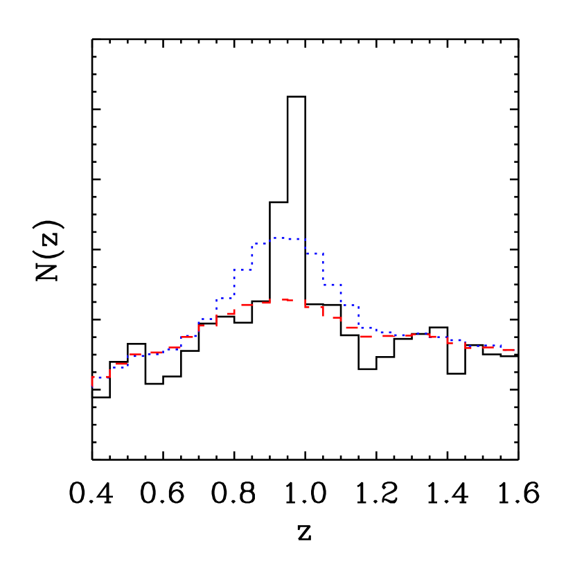
Figure 1.— The redshift distribution of nearby neighbors of objects drawn from a lightcone based on the Millennium Simulation. We select objects at $0.9<z<1.0$ and plot the redshift distribution of all neighbors (chosen, in this case, to have an angular separation $2.5\arcsec<\theta<15\arcsec$ from the central object) as the black histogram. The spike shows that a significant number of the nearby neighbors lie at the same redshift as the central objects. The blue dotted histogram has been calculated in the same way as the black histogram, except that the redshifts of all objects have been perturbed to simulate photometric redshifts; the spike is still visible, but has been broadened by the redshift errors. The red dashed histogram shows the redshift distribution of neighbors after randomizing the galaxy positions, and simply reflects the overall redshift distribution of all objects in the catalog; this can be taken as an estimate of the contribution to $N(z)$ of projected close pairs.

2.2. Estimating Photometric Redshift Accuracy from Physically-Associated Pairs

In the absence of spectroscopic redshifts, the dispersion of photometric redshifts can be estimated by comparing the difference in the photometric redshifts of the objects in physical pairs. To see how this is done, we model the photometric redshifts as being offset from the true redshifts using

$$z_{phot}=\delta_{z}\cdot(1+z)+z,$$ (1)

where $\delta_{z}$ is a random deviate. Eq. 1 implicitly assumes that the uncertainties are constant in units of $(1+z)$ — but note that this condition is at best only approximately met in current data sets. Since typical photometric redshift uncertainties are significantly larger than the true redshift differences in physically-associated pairs, we can assume that the true redshifts of both objects in a pair are identical.

The best estimate of the true redshift of a pair is its mean photometric redshift. We can then measure the quantity

$$\Delta_{z}\equiv(z_{phot,1}-z_{phot,2})/(1+z_{mean}).$$ (2)

From eqs. 1 and 2, it can be shown that

$$\Delta_{z}\simeq\delta_{1}-\delta_{2}-\frac{1}{2}(\delta_{1}^{2}-\delta_{2}^{2}),$$ (3)

where we have kept only the first- and second-order terms. If $\delta_{z}$ follows a Gaussian distribution, and if $\delta_{z}<<1$, then the dispersion in $\Delta_{z}$ is related to the dispersion in $\delta_{z}$ by

$$\sigma(\Delta_{z})\simeq\sqrt{2}\sigma(\delta_{z}).$$ (4)

where we have additionally assumed that both objects in the pair have similar uncertainties. There may be times when it is useful to consider close pairs of different types of objects, such as bright-faint pairs, in which case this assumption will not hold and the uncertainties should be added in quadrature.

2.3. Subtracting out the Projected Pairs

Unless pairs with only very small angular separations are used, the number of projected pairs will be comparable to, or significantly greater than, the number of physical pairs. It then becomes necessary to statistically subtract out the contaminants. The expected number and distribution of contaminants can be easily estimated by randomizing the positions of the galaxies from which the observed pairs are drawn (while keeping the redshifts the same), and by detecting the random pairs. The random positions should follow the same observing geometry constraints as the observed positions (i.e. avoiding the locations of bright stars or other image artifacts), and the process can be repeated several times to reduce the uncertainty.

For purposes of illustration, we create “photometric redshifts” for objects in the lightcone by perturbing the true redshifts with Gaussian random deviates with $\sigma=0.06$, which is a typical error for high signal-to-noise objects in high-quality data sets at $z>1$. We select objects in the lightcone with $1<z_{phot}<2$, and identify all pairs with an angular separation 2.5–15$\arcsec$. The lower limit is applied to minimize the effect of blending on the object photometry (this is obviously not an issue for the simulated data used in this section, but will be an issue for actual data). The upper limit was chosen arbitrarily; a larger value would yield more pairs, and thus a more accurate estimate of the redshift uncertainties, but 15$\arcsec$ is sufficient for our purposes and limits the computational expense. The left panel of Fig. 2 shows the distribution of $\Delta z_{phot}/(1+z_{mean})$ for both the observed pairs and the pairs found in the randomized catalog. In the right panel we subtract the randomized histogram from the true histogram; this subtraction is a statistical correction for the projected pairs. Also shown is the best-fitting Gaussian, which has width $\sigma=0.084$, which is essentially identical to the expected value of $\sqrt{2}\cdot 0.06$ from eq. 4. .

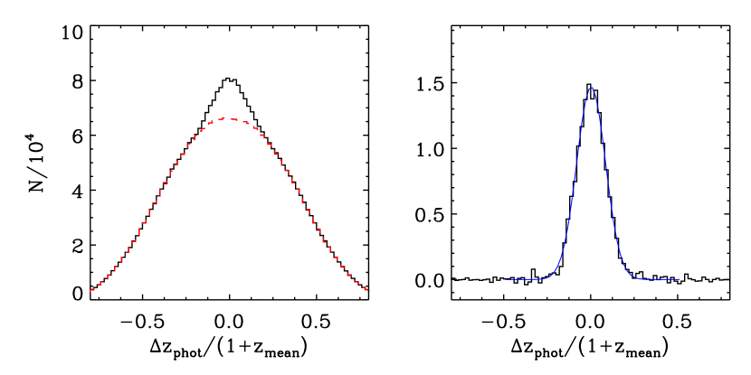
Figure 2.— Left: The black histogram shows the distribution of $\Delta z_{phot}/(1+z_{mean})$ for galaxy pairs selected with $1<z_{phot}<2$ in a simulated lightcone. The red histogram shows the same thing, but drawn from a catalog in which the galaxy positions have been randomized in order to estimate the distribution for chance projections. Right: The histogram shows an estimate of the distribution of redshift separations for physical galaxy pairs, which comes from subtracting the red histogram from the black histogram in the left panel. The blue curve shows the best-fitting Gaussian, which has a width that is greater than the photometric redshift errors by a factor of $\simeq\sqrt{2}$.

It can be numerically intensive to generate several random catalogs based on the actual data, and to identify all close pairs, as described above — especially if one wishes to repeat the measurements many times for different samples of galaxies. In practice we speed up the method by creating a single large catalog of points with random angular positions, detecting the pairs, and storing the vector of pair separations. Then we can quickly mimic the random catalogs described above for any range of angular separations by assigning to each value of the separation a value of $\Delta_{z}$, where the photometric redshifts in eq. 2 are drawn at random from the data. The remaining step is to scale the number of random pairs to the number there would be if the random catalog had the same number of objects as the data catalog.

2.4. Non-Gaussian Errors

In the previous sections we dealt with the case of Gaussian photometric redshift errors. But in actual data sets the average photometric redshift probability distribution will not generally be a perfect Gaussian, and hence $\Delta_{z}$ will also deviate from a Gaussian. It is therefore of interest to consider other functional forms, particularly those with more prominent wings than a simple Gaussian. One possibility is to consider the case of error distributions that are the sum of two Gaussians. We first note that the distribution of $z_{phot,1}-z_{phot,2}$ is simply the error distribution convolved with itself . A single Gaussian convolved with itself will become broader by a factor of $\sqrt{2}$, which explains presence of that factor in eq. 4. A double Gaussian convolved with itself results in a triple Gaussian (i.e. each of the two Gaussians convolved with themselves, plus a third Gaussian which is the two Gaussians convolved with each other).

To illustrate how this works, we produce “photometric redshifts” in the lightcone by perturbing the spectroscopic redshifts by a double Gaussian, with widths $\sigma_{1}=0.03$ and $\sigma_{2}=0.09$, and we set the relative areas of the second to the first Gaussian to $r=0.5$. This is the same as saying that $2/3$ of the objects have a redshift error given by $\sigma_{1}$ and $1/3$ have an error given by $\sigma_{2}$. We then calculate $\Delta(z_{phot})/(1+z_{mean})$ for the close pairs, and fit a function of the form

$$F(x)=AG(x,2\sigma_{1}^{2})+A2rG(x,\sigma_{1}^{2}+\sigma_{2}^{2})+Ar^{2}G(x,2\sigma_{2}^{2})$$ (5)

where $G(x,\sigma^{2})$ is a normalized Gaussian with variance $\sigma^{2}$, and $A$ is just an overall normalization factor. Thus the fitting parameters are $(A,\sigma_{1},\sigma_{2},r)$, and we have increased the number of parameters relative to the single Gaussian case by two.

Figure 3 shows the result. We obtain $(\sigma_{1},\sigma_{2},r)=(0.031,0.083,0.50)$, which is close to the input values. This figure also shows the result of fitting a single Gaussian to the distribution; the fit is obviously not as good, but still give a reasonable estimate of the errors, with $\sigma=0.06$. In practice, fits using eq. 5 can become somewhat unstable in certain regimes of parameter space due to covariance in the fitting parameters, or due to poor signal-to-noise. It is useful to constrain the fitting parameters so they do not reach very small, or negative, values.

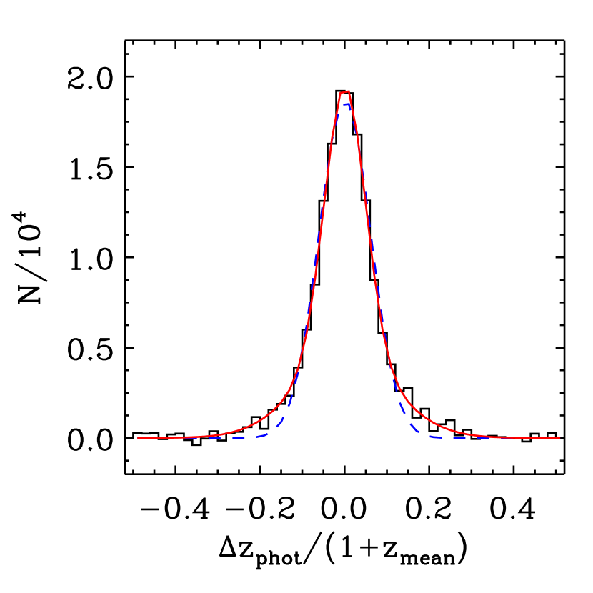
Figure 3.— The distribution of $\Delta z_{phot}/(1+z_{mean})$ after correcting for projected pairs. The photometric redshift errors have been parameterized as the sum of two Gaussians, so the appropriate fitting function for $\Delta z_{phot}/(1+z_{mean})$ is the sum of three Gaussians (see text). This fit is shown by the red curve. The dashed blue curve shows the result of a single Gaussian fit.

Another formula that is useful to parameterize photometric redshift errors in the case of non-Gaussian tails is the Lorentz distribution, $L(x,\gamma)$. Convolving a Lorentz distribution with itself results in another Lorentz distribution where $\gamma$ is increased by a factor of 2 (Dwass, 1985). So in this case the fitting function for $\Delta z_{phot}/(1+z_{mean})$ would be

$$F(x)=AL(x,2\gamma)$$ (6)

where the fitting parameters are $(A,\gamma)$.

2.5. Estimating the Catastrophic Failure Rate

Thus far we have modeled the photometric redshift errors as small perturbations on the true redshifts. However, actual photometric redshifts are subject to “catastrophic failures.” These outliers may be caused by multiple minima in $\chi^{2}(z)$, or may arise from a mismatch between the observed galaxy spectral energy distributions and the galaxy templates used when calculating photometric redshifts. It is possible to estimate the outlier rate by looking for an excess of neighbors with widely discrepant photometric redshifts (see also Erben et al., 2009, who use the cross-correlation between galaxies in different photometric redshift bins to detect the existence of catastrophic failures).

To demonstrate the effects of catastrophic failures, we first detect only the physical pairs in the lightcone. We then generate “photometric redshifts” for each object as described in § 2.3, but now include outliers by assigning random redshifts that are constrained to be at least $5\sigma$ away from the true redshift for $30\%$ of the objects (the catastrophic failure rate is lower than this for normal galaxies in current multiwavelength surveys, but we exaggerate the effect to provide a clear illustration). Figure 4 shows the result. The best-fitting Gaussian still has a width of $\sim\sqrt{2}\cdot 0.06$, but the distribution of $\Delta z_{phot}/(1+z_{mean})$ has broad wings due to the outliers.

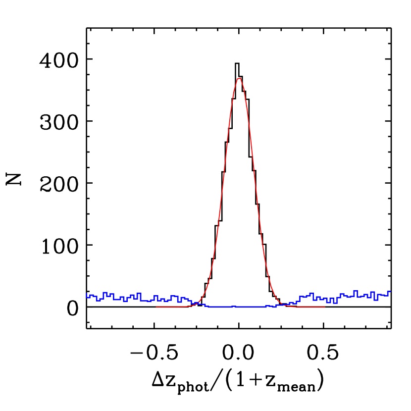
Figure 4.— The effect of catastrophic redshift failures. The black histogram shows the distribution of $\Delta z_{phot}/(1+z_{mean})$ for all physical galaxy pairs which have Gaussian photometric redshift errors in the simulations, while the blue histogram shows the contribution from pairs that contain at least one catastrophic failure. In this example the catastrophic outlier rate is $30\%$.

The outlier rate can be estimated from the area under the histogram at large $|\Delta z_{phot}|/(1+z_{mean})$. In this case, the fractional area at $|\Delta z_{phot}|/(1+z_{mean})>0.3$ is $30.4\%$, which is close to the expected value of $30\%$.

We note that the extended, flat wings shown in Figure 4 are due to the flat redshift distribution that we use for the redshift outliers. In actual data sets, the outliers will frequently not have a flat redshift distribution, for instance because of the double redshift solutions which can be caused by confusion between the Lyman and Balmer/4000Å breaks. Nevertheless, this example illustrates that even the central part of the distribution of $\Delta z_{phot}/(1+z_{mean})$ can be affected by the outliers (where the blue and red histograms overlap in Figure 4), so it is important to fit a Gaussian only over the regions that are clearly dominated by non-outliers. The location of this region will depend on what is chosen to constitute a catastrophic failure. In practice, the catastrophic failure rate can not always be tightly constrained, and relies on accurate modeling of the projected pairs.

3. The Effects of Systematic Errors in the Photometric Redshifts

In the previous section we demonstrated the close-pairs technique on mock data. Here we use the technique to determine the photometric redshift errors in an actual dataset, and discuss the effects of systematic redshift errors.

The Cosmic Evolution Survey (COSMOS; Scoville et al., 2007) is a 2 deg² multiwavelength survey, and was conducted with the primary goal of studying the relationship between galaxy evolution and large-scale structure. A unique aspect of this survey is the number of observed filters, with 30 bands from the ultra-violet to the mid-infrared. Particularly valuable is the deep medium-band optical imaging, which traces galaxy spectral energy distributions with much higher resolution than is possible with standard broadband filters. Ilbert et al. (2009) present photometric redshifts for the COSMOS field. They use a template-fitting approach to derive the photometric redshifts, paying particular attention to the choice of templates and to the effects of emission lines. The medium-band imaging allows Ilbert et al. (2009) to achieve extremely accurate photometric redshifts out to $z\sim 1$; for the brightest sources, with $I<22.5$, they quote a typical error in $|\Delta(z)|/(1+z)$ of 0.007.

Another unique aspect of this field is the large number of spectroscopic redshifts available from the zCOSMOS survey (Lilly et al., 2009). For the purposes of this paper, these spectroscopic redshifts are extremely useful as the zCOSMOS-bright sample has a high level of completeness for $I<22.5$, and the objects with secure spectroscopic redshifts are a relatively unbiased subset of the parent population. Thus we can use these spectroscopic redshifts to obtain an independent test of the photometric redshift errors. In what follows, we reject objects classified as stars or x-ray sources in the photometric catalog. We also only make use of the secure spectroscopic redshifts (with confidence class 3 or 4).

To demonstrate how well we can recover the photometric redshift errors from real data using the technique described in this paper, we begin by comparing our estimate of the errors to a direct measurement of the errors made by comparing photometric and spectroscopic redshifts for individual galaxies. For this we use the zCOSMOS-bright sample. The left panel in Figure 5 shows the $\Delta z_{phot}/(1+z_{mean})$ for galaxies with $17.5<I<22.5$. The blue curve shows the best fit, using the fitting function eq. 5. The right panel shows the direct measurement of the photometric redshift errors in a standard $(z_{phot}-z_{spec})/(1+z_{spec})$ plot, and the blue curve shows the predicted errors from the fit in the left panel. Although to first order we do recover the typical magnitude of the errors reasonably well, the distribution of errors is obviously not perfect as the central region is too strongly peaked.

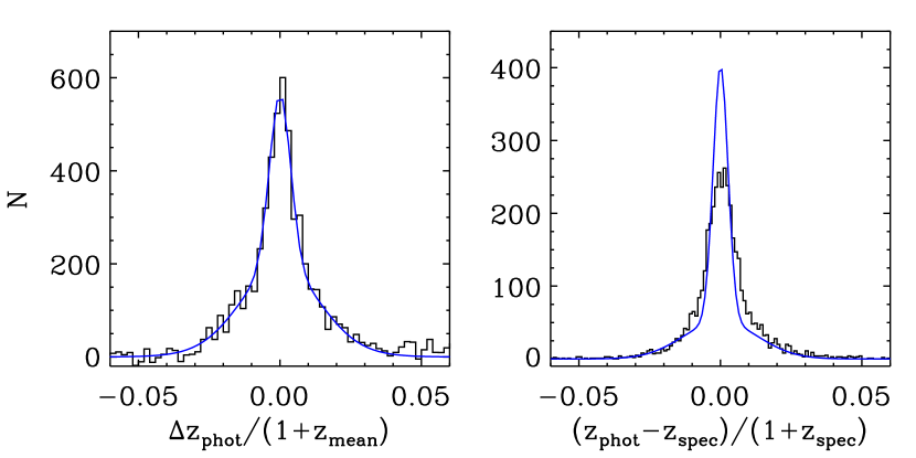
Figure 5.— Left: The distribution of $\Delta z_{phot}/(1+z_{mean})$ for galaxies with $17.5<I<22.5$ in the COSMOS field. The blue curve is a fit. Right: The distribution of $(z_{phot}-z_{spec})/(1+z_{spec})$ for objects with spectroscopic redshifts from zCOSMOS, again for galaxies with $17.5<I<22.5$. The curve is the error distribution that would be inferred from the fit in the left panel. Although the typical size of the errors is recovered well to first order, the shape of the error distribution is not perfect.

This effect can be seen more strongly at fainter magnitudes, as demonstrated in Figure 6. The left panel shows $\Delta z_{phot}/(1+z_{mean})$ for galaxies with $24<I<25$. Here the error distribution appears highly non-Gaussian, with broad tails and a very narrow peak. In this case we cannot directly measure the photometric redshift errors as done in Figure 5 since there are few spectroscopic redshifts available for galaxies at these faint magnitudes. Thus we follow a different approach of estimating the error distribution from photometric-spectroscopic pairs, i.e. we measure the redshift separation of close pairs where one object has a spectroscopic redshift from the zCOSMOS-bright sample and the other object has $24<I<25$. In this case, the projected pairs can be subtracted out in a manner analogous to that described in §2.3, except that the positions of spectroscopic sample are fixed and only the positions of the photometric sample are randomized. The photometric redshift errors estimated in this way are shown in the right panel of Figure 6. Again, the solid blue curve shows the error distribution that would have been predicted from the fit in the left panel. Obviously, the strong central peak is an artifact and does not represent the true errors. The red dashed curve in this panel is a fit using a double-Gaussian fitting function, and the red curve in the left panel shows the resulting prediction for $\Delta z_{phot}/(1+z_{mean})$ .

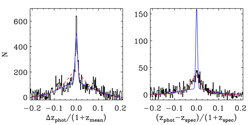
Figure 6.— Left: The distribution of $\Delta z_{phot}/(1+z_{mean})$ for galaxies with $24<I<25$ in the COSMOS field. The solid blue curve is a fit. Right: The distribution of $(z_{phot}-z_{spec})/(1+z_{spec})$ for pairs of objects with one photometric and one spectroscopic redshift (see text). The solid blue curve is the error distribution that would be inferred from the fit in the left panel. The dashed red curve is a fit to the data in this panel, and the dashed red curve in the left panel is the corresponding prediction for $\Delta z_{phot}/(1+z_{mean})$. The differences between the red and blue curves in both of these panels illustrates the effect of photometric redshift “attractors,” which is substantial for faint galaxies in the COSMOS photometric redshift catalog.

The fact that many close pairs of objects have photometric redshifts that are closer than expected based on the true errors is largely due to an artifact of the photometric redshift algorithm. It is a common feature of many data sets that there are artificial spikes in the photometric redshift distribution. These spikes may result from the particular filter/template combination, or may be due to systematic errors in object colors. For instance, if the observed galaxy colors in two closely-spaced filters are systematically too red — due to poor PSF matching or zeropoint errors — then the photometric redshift code may interpret the red colors as being due to 4000Å breaks in the galaxy SEDs, with the effect that many objects will have artificially similar photometric redshifts.

This illustrates the fundamental limitation of the technique described in this paper, which is that its usefulness is reduced in the case of significant systematic redshift errors. A more frequently-discussed type of systematic error, in which all photometric redshifts are over- or underestimated, will go completely undetected using the method described in §2 (however in some cases such biases are relatively unimportant, so long as they are small; Quadri et al., 2007). Artificial spikes in the photometric redshift distribution are a somewhat different type of systematic error; this type of error is not nearly as noticeable in most data sets as it is in Figure 6, and we have made use of the COSMOS field here primarily for its illustrative value. This does not necessarily mean that the COSMOS photometric redshifts suffer from redshift “attractors” — also sometimes called “redshift focusing” — more than other photometric redshift catalogs; it may simply mean that the random errors are so small in this case that the systematic errors become important.

4. Differential Photometric Redshift Errors

In this section we investigate how photometric redshift errors depend on redshift, signal-to-noise ratio (S/N), and galaxy type. Because in most data sets the photometric redshifts are constrained primarily by the locations of Lyman break and/or the Balmer/4000Å break, objects with weak or undetected breaks will have comparatively uncertain photometric redshifts. It is therefore expected that redshift accuracy will depend not just on galaxy brightness, but also on galaxy type.

Here we use public data in the field observed by the UKIDSS Ultra-Deep Survey (UDS; Lawrence et al., 2007; Warren et al., 2007). We use an updated version of the UDS catalog that was presented by (Williams et al., 2009), and details of the data, photometry, and redshifts can be found in that work. Briefly, this catalog includes near-infrared (NIR) imaging from the UDS, optical imaging from the Subaru-XMM Deep Survey (SXDS; Furusawa et al., 2008), and infrared imaging from the Spitzer Wide-Area Infrared Extragalactic Survey (SWIRE; Lonsdale et al., 2003). The field size with complete multiwavelength coverage is $\sim$0.65$\rm{deg}^{2}$. The latest version of our catalog includes $H$-band imaging in the NIR from the UDS data release 3 and $V$-band imaging from the SXDS data release 1. We have also added $u^{*}$-band imaging from the Canada-France Hawaii Telescope (CFHT) that was taken as part of Program ID #07BC25 (P.I. O. Almaini), and was downloaded from the CFHT archive. Those data were kindly reduced for us by H. Hildebrandt using the procedures described in Erben et al. (2009) and Hildebrandt et al. (2009). Thus the updated catalog has complete $u^{*}BVRi^{\prime}z^{\prime}JHK3.6\mu\rm{m}4.5\mu\rm{m}$ photometry.

The photometric redshifts were calculated from the updated catalog using the EAZY code (Brammer, van Dokkum, & Coppi, 2008). We did not perform any tuning of the default EAZY parameters, with the single exception of reducing the amplitude of the template error function to 0.5, which has been found to provide better results in several different data sets (G. Brammer, private communication). Additionally we use an updated template set with a new treatment of emission lines (Brammer et al., in prep.).

To illustrate the effect of galaxy type on redshift accuracy, we separate galaxies into star-forming and quiescent populations according to the bimodality in a rest-frame $U-V$ vs. $V-J$ color-color diagram (Williams et al., 2009). We limit the sample to $K<22.9$, and reject galaxies with high $\chi^{2}$ values from the template fits as those objects tend to have very inaccurate photometric redshifts and are frequently AGN.

We estimate accuracy in $\Delta(z)/(1+z)$ in four redshift bins: $0.3<z_{phot}<0.7$, $0.7<z_{phot}<1.2$, $1.2<z_{phot}<1.7$, and $1.7<z_{phot}<2.2$. Within each redshift bin, we separate galaxies into a bright and faint subsample according to the median signal-to-noise ratio (S/N) of all galaxies in that bin. Although most studies classify galaxies according to the S/N in the detection band, it is not obvious that this is a relevant statistic. In this case, the detection band is $K$, which does not actually play a major role in constraining the redshifts at $z<2$. Since photometric redshifts are most strongly constrained at these redshifts by the identification of the 4000Å break, we use the S/N in the closest band redward of the break. Thus an old galaxy with a strong break, which may have high S/N redward of the break and low S/N blueward of the break, will be appropriately classified as high S/N since the location of the break will be tightly-constrained.

For each galaxy sample, we fit the distribution of $\Delta z_{phot}/(1+z_{mean})$ using eq. 5. Figure 7 shows the result in the $1.2<z_{phot}<1.7$ redshift bin (without splitting the samples by S/N). It is immediately apparent that the quiescent galaxies have more accurate redshifts than the star-forming galaxies. This is more clearly demonstrated in Figure 8, which shows the $68\%$ uncertainty in $\Delta(z)/(1+z)$ that we estimate by integrating the inferred photometric redshift error distribution. The red and blue solid curve show how this quantity changes with redshift for the quiescent and star-forming galaxies, respectively. The upper and lower dashed curves show the accuracy for the fainter and brighter subsamples of each population.

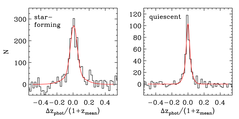
Figure 7.— The distribution of $\Delta z_{phot}/(1+z_{mean})$ for star-forming galaxies and quiescent galaxies at $1.2<z_{phot}<1.7$ in the UDS. The quiescent galaxies have more accurate photometric redshifts.

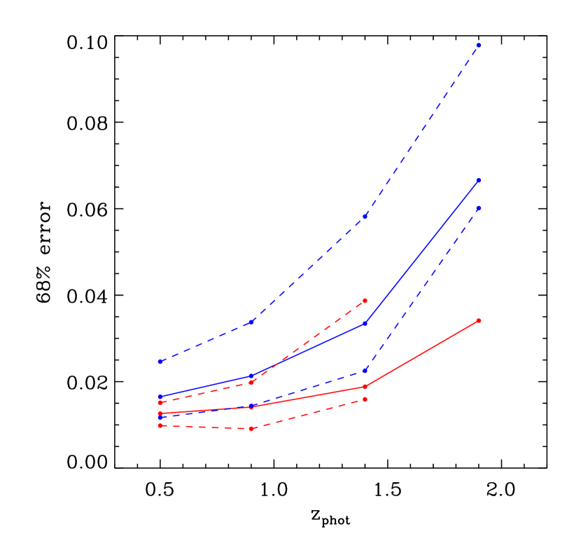
Figure 8.— The $68\%$ errors in $\Delta(z)/(1+z)$ as function of redshift for star-forming (blue curves) and quiescent (red curves) galaxies. The solid curves are for the full sample of $K<22.9$ objects, while the lower dashed curves are for bright galaxies and the upper dashed curves are for faint galaxies. A galaxy is classified as bright (faint) if the S/N in the band immediately redward of the 4000Å break is higher (lower) than the median for all galaxies in that redshift bin.

The quality of the photometric redshifts in the UDS is impressively good. The quiescent galaxies, in particular, have extremely accurate redshifts at $z\lesssim 1$. This is confirmed by a direct comparison of photometric with spectroscopic redshifts using the substantial spectroscopic sample of $z\sim 1$ passively-evolving galaxies from Yamada et al. (2005); this yields $\Delta(z)/(1+z)=0.015$, in good agreement with the results shown in Figure 8.

The quiescent galaxies do show significantly more accurate photometric redshifts than the star-forming galaxies over all redshifts probed here. For certain types of studies, such differential photometric redshift errors can adversely affect the results. For instance, the increased errors for star-forming galaxies can lower the inferred correlation length (Quadri et al., 2007), leading to an artificial trend of clustering with star formation properties. Another example is the mass/luminosity function: redshift errors will tend to flatten these functions relative to their true values (Chen et al. 2003; but see Marchesini et al. 2007), and can lead to an artificial difference between these functions for star-forming and quiescent galaxies.

The result that quiescent galaxies have more accurate redshifts is obviously somewhat dependent on image depth and filter coverage; our deep images and closely-spaced optical and NIR filters allow us to pinpoint the location of the Balmer/4000Å break for quiescent galaxies quite accurately, while the lack of ultra-violet imaging means that we cannot detect the Lyman break of star-forming galaxies at these redshifts. It is entirely possible that with different data the star-forming galaxies would have photometric redshift accuracy comparable to, or even better than, the quiescent galaxies.

5. Summary and Discussion

The use of photometric, as opposed to spectroscopic, redshifts makes it possible to study a much larger number of objects for a given amount of telescope time. But photometric redshift errors will propagate through many different types of analyses, and in practice may comprise a significant source of error in derived quantities. For this reason a realistic estimate of the distribution of photometric redshift errors is necessary. Obtaining large, representative samples of spectroscopic redshifts with which to directly measure the photometric redshift errors is observationally expensive, and often completely unfeasible. For this reason it is of great interest to have a method to estimate the size and distribution of such errors that can be applied with limited, or even non-existent, spectroscopic samples.

In this paper we have presented such a method. It is based on the idea that a close association of two or more galaxies on the sky may represent a true physical association, in which case the objects will lie at nearly the same redshift and the differences between their photometric redshifts constrains the typical errors. We have described a simple implementation of this idea that makes use of close galaxy pairs, where the best estimate of the true redshift of a pair is taken to be the mean of the photometric redshifts. We have described how to estimate the photometric redshift error distribution from the difference in photometric redshifts, as well as how to estimate the catastrophic failure rate. This technique requires applying a statistical correction for pairs that arise from chance projections along the line of sight, and this is easily done by randomizing the galaxy positions and repeating the analysis. Although in this paper we have focused on the redshift range $0.5\lesssim z\lesssim 2$, the basic technique can be applied at both significantly lower and higher redshifts.

The concept of using angular associations between galaxies to constrain their redshifts is not entirely new. Newman (2008) uses a cross-correlation between a spectroscopic and a photometric sample of galaxies to infer the true redshift distribution of the photometric sample. Erben et al. (2009) uses the cross-correlation between galaxies selected in two disjoint photometric redshift bins to quantify the photometric redshift errors. Kovac et al. (2009) modifies the photometric redshift probability distribution of objects on the basis of the spectroscopic redshifts of nearby objects. The technique presented in this paper represents a significant step forward because it is simple to implement, the results are easy to interpert, and it can be applied with limited (or even with a complete lack of) spectroscopic information.

As a first application of our method, we have shown that quiescent galaxies will on average have more accurate photometric redshifts than star-forming galaxies in broadband optical/NIR surveys out to at least $z\sim 2$. This is because quiescent galaxies have a strong break in their SEDs near 4000Å, and if the location of this break can be pinpointed using the observed photometry, the redshift will be tightly constrained. Star-forming galaxies, on the other hand, have weaker features in their SEDs over the range of observed wavelengths. Differential photometric redshift errors can lead to differential effects in derived quantities, such as luminosity or mass functions, and should be taken into account when comparing such quantities between samples.

A significant limitation of the method presented in this paper arises from systematic errors in the photometric redshifts. One type of systematic error, in which all photometric redshifts are biased in one direction, will go completely undetected. However if a particular class of galaxies (e.g. galaxies on the red sequence) is subject to such a bias, whereas another class (in the blue cloud) is not, then this bias will become apparent by looking at cross-pairs (red-blue pairs). Another type of systematic error is when the photometric redshift distribution shows artificial spikes. This is particularly problematic, as it means that the photometric redshifts of a pair of objects may both be drawn into the spike, leading to a smaller relative redshift difference and an underestimate of the true redshift errors. In extreme cases, when this type of error is comparable to the random errors, this effect can lead to highly disturbed error distributions (Fig. 6). Both of these types of systematic errors can, however, be accounted for by using pairs where one object has a known spectroscopic redshift.

In principle the results from the close-pairs technique may be subject to subtle biases related to the relationship between galaxy properties and local environment. For instance, if red sequence galaxies preferentially appear in groups, then they will be over-represented in a sample of close pairs. Similarly, galaxies with boosted star formation due to close interactions may also be over-represented. On the other hand, such galaxies may be relatively rare, and it is worthwhile to remember that the number of pairs in a sample is a strong function of the sample size itself, growing like $N^{2}-N$. Another potential problem is that close pairs of objects may have inaccurate photometry due to blending or poor background subtraction, so it is important to apply a sensible lower limit for the pair separations.

Our method of using angular associations of galaxies to constrain both the redshifts and the redshift errors can be applied and extended in various ways. Particularly intriguing is the possibility of incorporating information from angular associations directly into photometric redshift codes. A step in this direction has already been taken by Kovac et al. (2009), who modify the photometric redshift probability distributions of objects that have near neighbors with spectroscopic redshifts; here we simply note that this same idea may be extended to neighbors with only photometric information. Regardless of how the ideas discussed in this paper are used in future, the close-pairs technique is straightforward to apply and should prove to be a useful tool in analyzing data from redshift surveys.

References

- Adelberger (2005) Adelberger, K. 2005, ApJ, 621, 574
- Albrecht et al. (2006) Albrecht, A., et al. 2006, arXiv:astro-ph/0609591
- Bolzonella, Miralles, & Pelló (2000) Bolzonella, M., Miralles, J.-M., & Pelló, R. 2000, A&A, 363, 476
- Brammer, van Dokkum, & Coppi (2008) Brammer, G. B., van Dokkum, P. G., & Coppi, P. 2008, ApJ, 686, 1503
- Chen et al. (2003) Chen, H.-W., et al. 2003, ApJ, 586, 745
- Dwass (1985) Dwass, M. 1985, American Mathematical Monthly, 92, 55.
- Erben et al. (2009) Erben, T., et al. 2009, A&A, 493, 1197
- Collister & Lahav (2004) Collister, A. A., & Lahav, O. 2004, PASP, 116, 345
- Furusawa et al. (2008) Furusawa, H., et al. 2008, ApJS, 176, 1
- Hildebrandt et al. (2009) Hildebrandt, H., Pielorz, J., Erben, T., van Waerbeke, L., Simon, P., & Capak, P. 2009, A&A, 408, 725
- Huterer et al. (2006) Huterer, D., Takada, M., Bernstein, G., & Jain, B. 2006, MNRAS, 366, 101
- Ilbert et al. (2009) Ilbert, O., et al. 2009, ApJ, 690, 1236
- Kovac et al. (2009) Kovac, K., et al. 2009, ApJ, submitted (arXiv: 0909.3409)
- Kitzbichler & White (2007) Kitzbichler, M. G., & White, S. D. M. 2007, MNRAS, 376, 2
- Lilly et al. (2009) Lilly, S. J., et al. 2009, ApJS, 184, 218
- Lawrence et al. (2007) Lawrence, A., et al. 2007, MNRAS, 379, 1599
- Lonsdale et al. (2003) Lonsdale, C. J., et al. 2003, PASP, 115, 897
- Mandelbaum et al. (2008) Mandelbaum, R., et al. 2008, MNRAS, 781, 806
- Marchesini et al. (2007) Marchesini, D., et al. 2007, ApJ, 656, 42
- Newman (2008) Newman, J. A. 2008, ApJ, 684, 88
- Quadri et al. (2007) Quadri, R., et al. 2007, ApJ, 654, 138
- Quadri et al. (2008) Quadri, R. F., et al. 2008, ApJ, 685, L1
- Scoville et al. (2007) Scoville, N., et al. 2007, ApJS, 172, 1
- Springel et al. (2005) Springel, V. 2005, Nature, 435, 629
- Warren et al. (2007) Warren, S. J., et al. 2007, MNRAS, 375, 213
- Williams et al. (2009) Williams, R. J., Quadri, R. F., Franx, M., van Dokkum, P., & Labbé, I. 2009, ApJ, 691, 1879
- Yamada et al. (2005) Yamada, T., et al. 2005, ApJ, 634, 861