Laurent polynomial moment problem:
a case study

Abstract

In recent years, the so-called polynomial moment problem, motivated by the classical Poincaré center-focus problem, was thoroughly studied, and the answers to the main questions have been found. The study of a similar problem for rational functions is still at its very beginning. In this paper, we make certain progress in this direction; namely, we construct an example of a Laurent polynomial for which the solutions of the corresponding moment problem behave in a significantly more complicated way than it would be possible for a polynomial.

1 Introduction

The main result of this paper is a construction of a particular Laurent polynomial with certain unusual properties. This Laurent polynomial is a counterexample to an idea that, so far as the moment problem is concerned, rational functions would behave in the same way as polynomials. The main interest of the paper, besides the result itself, lies in a peculiar combination of methods which involve certainly the complex functions theory but also group representations, Galois theory, and the theory of Belyi functions and “dessins d’enfants”, while the motivation for the study comes from differential equations.

In addition to theoretical considerations our project involves computer calculations. It would be difficult to present here all the details. However, we tried to supply an interested reader with sufficient number of indications in order for him or her to be able to reproduce our results. A less interested reader may omit certain parts of the text and just take our word for it.

About a decade ago, M. Briskin, J.-P. Françoise, and Y. Yomdin in a series of papers [2]–[5] posed the following

Polynomial moment problem.

For a given complex polynomial $P$ and distinct complex numbers $a,b$, describe all polynomials $Q$ such that

$$\int^{b}_{a}P^{i}\,dQ\,=\,0$$ (1)

for all integer $i\geq 0$.

The polynomial moment problem is closely related to the center problem for the Abel differential equation in the complex domain, which in its turn may be considered as a simplified version of the classical Poincaré center-focus problem for polynomial vector fields. The center problem for the Abel equation and the polynomial moment problem have been studied in many recent papers (see, e. g., [1]–[8], [10], [13]–[23]).

There is a natural sufficient condition for a polynomial $Q$ to satisfy (1). Namely, suppose that there exist polynomials $\widetilde{P}$, $\widetilde{Q}$, and $W$ such that

$$P=\widetilde{P}\circ W,\qquad Q=\widetilde{Q}\circ W,\qquad\mbox{and}\qquad W(a)=W(b),$$ (2)

where the symbol $\circ$ denotes a superposition of functions: $f_{1}\circ f_{2}=f_{1}(f_{2})$. Then, after a change of variables $z\to W(z)$ the integrals in (1) are transformed to the integrals

$$\int^{W(b)}_{W(a)}\widetilde{P}^{i}\,d\widetilde{Q}$$ (3)

and therefore vanish since the polynomials $\widetilde{P}^{i}$ and $\widetilde{Q}$ are analytic functions in ${\mathbb{C}}$ and the integration path in (3) is closed. A solution of (1) for which (2) holds is called reducible. For “generic” collections $P$, $a$, $b$ any solution of (1) turns out to be reducible. For instance, this is true if $a$ and $b$ are not critical points of $P$, see [10], or if $P$ is indecomposable, that is, if it cannot be represented as a superposition of two polynomials of degree greater than one, see [15] (in this case (2) reduces to the equalities $P=W$, $Q=\widetilde{Q}\circ P$, and $P(a)=P(b)$). Nevertheless, as it was shown in [14], if $P(z)$ has several composition factors $W$ such that $W(a)=W(b)$ then the sum of the corresponding reducible solutions may be an irreducible one.

It was conjectured in [16] that actually any solution of (1) can be represented as a sum of reducible ones. Recently this conjecture was proved in [13]. The proof relies on two key components. The first one is a result of [17] which states that $Q$ satisfies (1) if and only if the superpositions of $Q$ with branches $P_{i}^{-1}(z)$, $1\leq i\leq n$, of the algebraic function $P^{-1}(z)$ satisfy a certain system of linear equations

$$\sum_{i=1}^{n}f_{s,i}Q(P^{-1}_{i}(z))=0,\ \ \ \ \ \ f_{s,i}\in{\mathbb{Z}},\ \ \ \ \ \ 1\leq s\leq k,$$ (4)

associated to the triple $P$, $a$, $b$ in effective way.

The second key componenet is related to the vector subspace $V_{P,a,b}\subset\mathbb{Q}^{n}$ spanned by the vectors

$$(f_{s,\sigma(1)},f_{s,\sigma(2)},\,...\,,f_{s,\sigma(n)}),\qquad 1\leq s\leq k,\qquad\sigma\in G_{P}\,,$$

where $G_{P}$ is the monodromy group of $P$ and $f_{s},$ $1\leq s\leq k,$ are vectors from (4). By construction, the subspace $V_{P,a,b}$ is invariant under the action of $G_{P}$, so the idea is to obtain a full description of such subspaces. In short, it was proved in [13] that if a transitive permutation group $G\leq{\rm S}_{n}$ contains a cycle of length $n$ then the decomposition of $\mathbb{Q}^{n}$ in irreducible components of the action of $G$ depends only on the imprimitivity systems of $G$. Obviously, the monodromy group of a polynomial of degree $n$ always contains a cycle of length $n$ which corresponds to the loop around infinity. Furthermore, imprimitivity systems of $G_{P}$ correspond to functional decompositions of $P$. Therefore, the structure of invariant subspaces of the permutation representation of $G_{P}$ over ${\mathbb{Q}}$ depends only on the structure of functional decompositions of $P$, and a careful analysis of system (4) and of the associated space $V_{P,a,b}$ eventually permits to prove that any solution of (1) is a sum of reducible solutions. Notice that using the decomposition theory of polynomials one can also show that actually any solution of (1) may be represented as a sum of at most two reducible solutions, and describe these solutions in a very explicit form (see [20]).

For example, in the simplest case of the problem corresponding to an indecomposable polynomial $P$ the above strategy works as follows. The only invariant subspaces of the permutation representation of $G_{P}$ on ${\mathbb{Q}}^{n}$ in this case are the subspace $V_{1}$ spanned by the vector $(1,1,\dots,1)$, and its complement $V_{1}^{\bot}$. Since system (4) contains an equation whose coefficients are not all equal this implies that $V_{P,a,b}=V_{1}^{\bot}$ and therefore (4) yields that

$$Q(P^{-1}_{1}(z))=Q(P^{-1}_{2}(z))=\dots=Q(P^{-1}_{n}(z))$$

identically over $z$. On the other hand, such an equality is possible only if $Q=\widetilde{Q}\circ P$ for some $\widetilde{Q}\in{\mathbb{C}}[z]$. Finally, $P(a)=P(b)$ since otherwise after the change of variables $z\rightarrow P(z)$ we would obtain that $\widetilde{Q}$ is orthogonal to all powers of $z$ on $[P(a),P(b)]$ in contradiction to the Weierstrass theorem.

In the paper [19] the following generalization of the polynomial moment problem was investigated: for a given rational function $F$ and a curve $\gamma\subset{\mathbb{C}}{\mathbb{P}}^{1}$, describe rational functions $H$ such that

$$\int_{\gamma}F^{i}\,dH\,=\,0$$ (5)

for all $i\geq 0$. In particular, in [19] another version of system (4) was constructed: its solutions, instead of the equality (5), guarantee only the rationality of the generating function $f(t)=\sum_{i=0}^{\infty}m_{i}t^{i}$ for the moments

$$m_{i}=\int_{\gamma}F^{i}\,dH\,.$$ (6)

On the other hand, it was shown that if the additional conditions $H^{-1}\{\infty\}\subseteq F^{-1}\{\infty\}$ and $F(\infty)=\infty$ are satisfied, then the rationality of $f(t)$ actually implies that $f(t)\equiv 0$.

The following modification of (2) is a natural sufficient condition implying (5): there exist rational functions $\widetilde{F}$, $\widetilde{H}$, and $W$ such that

$$F\,=\,\widetilde{F}\circ W,\qquad H\,=\,\widetilde{H}\circ W\,,$$ (7)

the curve $W(\gamma)$ is closed, and all the poles of the functions $\widetilde{F}$, $\widetilde{H}$ lie “outside” $W(\gamma)$ (the term “outside” is written in quotation marks since it is defined also for self-intersecting curves). We will call such a solution of (5) geometrically reducible. Notice that if $\gamma$ is closed then geometrically reducible solutions always exist. Indeed, one may take

$$W\,=\,F,\qquad H\,=\,\widetilde{H}\circ F$$

where $\widetilde{H}$ is any rational function with all its poles outside the curve $F(\gamma)$. It is also shown in [19] that, similarly to the case of a polynomial $P$, for a generic rational function $F$ (for example, for an $F$ whose monodromy group is the full symmetric group) all solutions of (5) turn out to be geometrically reducible. However, for a non-generic $F$ the situation becomes much more complicated in comparison with the polynomial moment problem, and some reasonable description of solutions of (5) seems (at least for the moment) to be unachievable.

In this paper we will consider a particular case of problem (5) which is especially interesting in view of its connection with the classical version of the Poincaré center-focus problem. Namely, we will consider the following

Laurent polynomial moment problem.

For a given Laurent polynomial $L$ which is not a polynomial in $z$ or in $1/z$, describe all Laurent polynomials $Q$ such that

$$\int_{S^{1}}L^{i}\,dQ\,=\,0$$ (8)

for all integer $i\geq 0$.

In contrast to the polynomial moment problem, not any solution of the Laurent polynomial moment problem is a sum of geometrically reducible solutions. For example, as it was observed in [19], if $L(z)=\widetilde{L}(z^{d})$ for some $d>1$, then the residue calculation shows that condition (8) is satisfied for any Laurent polynomial $Q$ containing no terms of degrees which are multiples of $d$. We will call such a solution of the Laurent polynomial moment problem algebraically reducible. Notice that, in distinction to geometrically reducible solutions which always exist, algebraically reducible solutions exist only if $L$ is decomposable and has $z^{d}$ as its right composition factor. One might think that any solution of the Laurent polynomial moment problem is a sum of geometrically and/or algebraically reducible solutions but, as we will see below, this is not the case either, although it seems that for a “majority” of Laurent polynomials $L$ this is the case.

It is natural to start the investigation of the Laurent polynomial moment problem by the study of the particular case where $L$ is indecomposable. At least, in this case there exist no algebraically reducible solutions. On the other hand, any geometrically reducible solution of (8) must have the form $Q=\widetilde{Q}\circ L$, where $\widetilde{Q}$ is a rational function whose poles lie outside the curve $L(S^{1})$. However, since $Q$ is a Laurent polynomial, it is easy to see that in this case $\widetilde{Q}$ is necessarily a polynomial. Furthermore, a sum of geometrically reducible solutions has the form

$$\sum_{i}\widetilde{Q}_{i}\circ L\,=\,\left(\sum_{i}\widetilde{Q}_{i}\right)\circ L$$

and hence is itself a geometrically reducible solution. Thus, “expectable” (and therefore not very interesting) solutions of the Laurent polynomial moment problem for indecomposable $L$ are of the form $Q=\widetilde{Q}(L),$ where $\widetilde{Q}$ is a polynomial. Any other solutions, when they exist, are of great interest since they show that the situation is more complicated than one might hope.

Let $L$ be an indecomposable Laurent polynomial of degree $n$, and let $G_{L}$ be its monodromy group. We will always assume that $L$ is proper, that is, it has poles both at zero and at infinity. In this case the group $G_{L}$ contains a permutation with two cycles: this permutation corresponds to the loop around infinity. Furthermore, it follows from Theorem 4.5 of [19] that if the only invariant subspaces of the permutation representation of $G_{L}$ on ${\mathbb{Q}}^{n}$ are $V_{1}$ and $V_{1}^{\bot}$, then any solution of the Laurent polynomial moment problem for $L$ is geometrically reducible. Therefore, if we want to find an example of a Laurent polynomial $L$ for which there exist solutions which are not geometrically reducible, we may use the following strategy:

• First, find a permutation group $G$ of degree $n$ such that $G$ would contain a permutation with two cycles, and the permutation representation of $G$ on ${\mathbb{Q}}^{n}$ would have more than two invariant subspaces.

• Then, realize $G$ as the monodromy group of a Laurent polynomial $L$.

• And, finally, prove somehow the existence of non-reducible solutions.

This program was started in [19]. Namely, basing on Riemann’s existence theorem it was shown that there exists a Laurent polynomial $L$ of degree 10 such that its monodromy group is permutation isomorphic to the action of ${\rm S}_{5}$ on two-element subsets of the set of 5 points. The corresponding permutation action of ${\rm S}_{5}$ on ${\mathbb{Q}}^{10}$ has more than two invariant subspaces. Furthermore, proceeding from a general algebraic result of Girstmair [11] about linear relations between roots of algebraic equations it was shown that there exists a rational function $Q$ which is not a rational function in $L$ such that the generating function for the sequence of the moments

$$m_{i}=\int_{S^{1}}L^{i}\,dQ,\ \ \ i\geq 0$$

is rational (see Sec. 8.3 of [19]). However, the methods of [19] do not permit to find $L$ or $Q$ explicitly and tell us nothing about the structure of solutions of (8).

In this paper we provide a detailed analysis of the above example with the emphasis on the two following questions of a general nature:

• First, how to construct a Laurent polynomial $L$ starting from its monodromy group $G_{L}$?

• Second, how to describe solutions of (8) which are not geometrically reducible ?

We answer all these questions for the particular Laurent polynomial $L$ given below. Actually, we believe that our methods can be used in a more general situation too and can serve as a “case study” for further research concerning the Laurent polynomial moment problem.

The main result of this paper is an actual calculation of an indecomposable Laurent polynomial $L$ such that the corresponding moment problem has non-reducible solutions, and a complete description of these solutions. Namely, we show that for

$$L\,=\,\frac{K\left(z-1\right)^{6}\left(z-a\right)^{3}\left(z-b\right)}{{z}^{5}}\,,$$ (9)

where

$$K\,=\,{\frac{11}{216}}+{\frac{5}{216}}\,\sqrt{5},\qquad a\,=\,-\frac{3}{2}+\frac{1}{2}\,\sqrt{5},\qquad b\,=\,\frac{7}{2}-\frac{3}{2}\,\sqrt{5}\,,$$

there exist Laurent polynomials $Q_{0}=1$, $Q_{1},Q_{2},Q_{3},Q_{4}$ (we compute them explicitly in Sec. 4) such that the following statement holds:

Theorem 1.1.

A Laurent polynomial $Q$ is orthogonal to all powers of $L$ on $S^{1}$ if and only if $Q$ can be represented in the form

$$Q\,=\,\sum_{j=0}^{4}(R_{j}\circ L)\cdot Q_{j}$$

for some polynomials $R_{0},R_{1},R_{2},R_{3},R_{4}$.

In other words, solutions of the moment problem for $L$ form a 5-dimensional module over the ring of polynomials in $L$ (while in a generic case such a module is one-dimensional and is therefore composed of polynomials in $L$ and of nothing else). The choice of the basis $Q_{j}$ is not unique, but once a basis is chosen the above representation of $Q$ becomes unique.

The paper is organized as follows. In Sec. 2 we give a detailed description of the permutation action of ${\rm S}_{5}$ on ${\mathbb{Q}}^{10}$. In Sec. 3 we compute explicitly a Laurent polynomial $L$ whose monodromy group is permutation equivalent to this action. Finally, in Sec. 4 we determine the above mentioned Laurent polynomials $Q_{j}$ and prove Theorem 1.1.

Acknowledgments.

The first author is grateful to C. Christopher, J. L. Bravo, and M. Muzychuk for valuable discussions, and to the Max-Planck-Institut für Mathematik for hospitality. The second author is indebted to the Center for Advanced Studies in Mathematics of the Ben-Gurion University for the financial support during his Post Docorate at Ben-Gurion University. The first and the third authors wish to thank the International Centre for Mathematical Sciences (Edinburgh) for the possibility to discuss a preliminary version of this paper.

2 Permutation representation of ${\rm S}_{5}$ on ${\mathbb{Q}}^{10}$ with more than two invariant subspaces

Consider the complete graph $K_{5}=(V,E)$ having the vertex set $V=\{1,2,3,4,5\}$ and the edge set $E$ consisting of all the subsets of $V$ of size 2. The symmetric group ${\rm S}_{5}$ acts on $V$ and therefore also on $E$, and we thus obtain a transitive action of ${\rm S}_{5}$ of degree 10. Moreover, the homomorphism ${\rm S}_{5}\to{\rm S}_{10}$ is obviously injective. Let us identify the canonical basis

$$\vec{e}_{1} = (1,0,0,0,0,0,0,0,0,0)\,,$$

$$\vec{e}_{2} = (0,1,0,0,0,0,0,0,0,0)\,,$$

$$\vdots \vdots$$

$$\vec{e}_{10} = (0,0,0,0,0,0,0,0,0,1)$$

of the space ${\mathbb{Q}}^{10}$ with the set $E$. This identification may in principle be arbitrary but we have chosen the one which is more “readable”, see Fig. 1: the first five vectors are associated, in a cyclic way, to the sides of the pentagon, while the last five vectors are associated in the similar way to the sides of the inside pentagram.

Figure 1: The correspondence between the edges of the complete graph $K_{5}$ and the basis in ${\mathbb{Q}}^{10}$.

Associating to each element of ${\rm S}_{5}$ a $10\times 10$ permutation matrix corresponding to the action of this element on $E$ we obtain a permutation representation of ${\rm S}_{5}$ on ${\mathbb{Q}}^{10}$. Any permutation representation of any finite group always has at least two invariant subspaces: the subspace $U_{1}$ of dimension 1 spanned by the vector $\vec{\mathbf{1}}=(1,1,\ldots,1)$, and its orthogonal complement $U_{n-1}=U_{1}^{\perp}$ of dimension $n-1$ containing the vectors $(x_{1},x_{2},\ldots,x_{n})$ having $\sum_{i=1}^{n}x_{i}=0$. While the space $U_{1}$ is obviously irreducible, the space $U_{n-1}$ may be, or may not be irreducible. We will show that in our case it is reducible.

One of the ways to construct invariant subspaces in our example is to consider subsets of edges which are sent to one another by the action of ${\rm S}_{5}$ on the vertices. Let us take the fans $F_{i}\subset E$, $i=1,\ldots,5$, where $F_{i}$ is the set of edges of $K_{5}$ incident to the vertex $i$, see Fig. 2.

Figure 2: The fans $F_{i}$, that is, the sets of edges incident to the vertex $i=1,\ldots,5$.

Obviously, any permutation of the vertices sends fans to fans. Therefore, the vectors $\vec{v}_{i}=\sum_{u\in F_{i}}e_{u}$, or, more concretely,

$$\vec{v}_{1} = (1,0,0,0,1,1,0,0,1,0)\,,$$

$$\vec{v}_{2} = (1,1,0,0,0,0,1,0,0,1)\,,$$

$$\vec{v}_{3} = (0,1,1,0,0,1,0,1,0,0)\,,$$

$$\vec{v}_{4} = (0,0,1,1,0,0,1,0,1,0)\,,$$

$$\vec{v}_{5} = (0,0,0,1,1,0,0,1,0,1)$$

(the first five and the last five components of these vectors move cyclically) span an invariant subspace $F\subset{\mathbb{Q}}^{10}$. It is easy to verify that $F$ is 5-dimensional. Since every edge is contained in exactly two fans we have $\sum_{i=1}^{5}\vec{v}_{i}=(2,2,\ldots,2)$ and therefore $F$ contains $U_{1}$ as its subspace. The orthogonal complement of $U_{1}$ in $F$ is a 4-dimensional invariant subspace $U_{4}\subset{\mathbb{Q}}^{10}$. The vectors

$$\vec{v}_{2}-\vec{v}_{1} = (0,1,0,0,-1,-1,1,0,-1,1)\,,$$

$$\vec{v}_{3}-\vec{v}_{1} = (-1,1,1,0,-1,0,0,1,-1,0)\,,$$

$$\vec{v}_{4}-\vec{v}_{1} = (-1,0,1,1,-1,-1,1,0,0,0)\,,$$

$$\vec{v}_{5}-\vec{v}_{1} = (-1,0,0,1,0,-1,0,1,-1,1)\,,$$

each having equal number of ones and minus ones, are orthogonal to the vector $\vec{\mathbf{1}}$. They are linearly independent, and therefore they span $U_{4}$.

Another collection of subsets of $E$ which is stable under the action of ${\rm S}_{5}$ is the set of Hamiltonian cycles $H\subset E$, that is, cycles that visit each vertex exactly once. A Hamiltonian cycle in $K_{5}$ can be described by a 5-cycle $c\in{\rm S}_{5}$ which indicates in which order the vertices are visited; note that $c^{-1}$ describes the same Hamiltonian cycle since our graph is undirected. The complement $\overline{H}=E\setminus H$ is also a Hamiltonian cycle which corresponds to the permutation $c^{2}$ (or to its inverse $c^{-2}$). There are 24 cyclic permutations in ${\rm S}_{5}$; they give rise to 12 Hamiltonian cycles in $K_{5}$ which form 6 pairs of mutually complementary cycles: see Fig. 3.

Figure 3: Pairs of Hamiltonian cycles in $K_{5}$: the “positive” cycles $H_{i}$ are drawn in bold lines, while their complements, the “negative” cycles $\overline{H}_{i}$, are shown in thin lines.

The vectors ${\vec{w}}_{k}=\sum_{u\in H_{k}}e_{u}-\sum_{u\in\overline{H}_{k}}e_{u}$ or, more concretely,

$${\vec{w}}_{1} = (1,-1,1,-1,1,-1,1,1,-1,-1)\,,$$

$${\vec{w}}_{2} = (1,1,-1,1,-1,-1,-1,1,1,-1)\,,$$

$${\vec{w}}_{3} = (-1,1,1,-1,1,-1,-1,-1,1,1)\,,$$

$${\vec{w}}_{4} = (1,-1,1,1,-1,1,-1,-1,-1,1)\,,$$

$${\vec{w}}_{5} = (-1,1,-1,1,1,1,1,-1,-1,-1)\,,$$

$${\vec{w}}_{6} = (-1,-1,-1,-1,-1,1,1,1,1,1)\,,$$

(once again the first five and the last five components move cyclically) span an invariant subspace. Every edge of $K_{5}$ belongs to 3 “positive” Hamiltonian cycles and to 3 “negative” ones; therefore, $\sum_{i=1}^{6}{\vec{w}}_{i}=0$. It is easy to verify that the space $U_{5}$ spanned by these 6 vectors is in fact 5-dimensional. For every fan $F_{i}$ and for every pair $(H_{j},\overline{H}_{j})$, exactly two edges of $F_{i}$ belong to $H_{j}$, while the other two belong to $\overline{H}_{j}$. Therefore, $\vec{v}_{i}\perp{\vec{w}}_{j}$ for all $i,j$, so $U_{5}\perp F$ where, as before, $F=U_{1}\oplus U_{4}$.

Thus, we get a decomposition of ${\mathbb{Q}}^{10}$ into three invariant subspaces: ${\mathbb{Q}}^{10}=U_{1}\oplus U_{4}\oplus U_{5}$. We did not prove that the subspaces $U_{4}$ and $U_{5}$ are irreducible. The proof goes by some routine verification using the character table of ${\rm S}_{5}$. We omit the details since for our goal this fact is irrelevant: the only thing we wanted to show was the reducibility of the orthogonal complement $U_{1}^{\perp}=U_{9}$, and this statement is proved since we have shown that $U_{9}=U_{4}\oplus U_{5}$.

We finish this section by specifying how certain elements of ${\rm S}_{5}$ act on the labels of the 10 edges. By construction, the permutation $f=(1,2,3,4,5)\in{\rm S}_{5}$ acts as

$$\varphi=(1,2,3,4,5)(6,7,8,9,10)\,.$$

Taking a simple transposition, for example, $a=(2,5)\in{\rm S}_{5}$, we get

$$\alpha=(1,5)(2,8)(4,7)\,.$$

Indeed, all the edges having both ends different from 2 and 5, remain fixed, as well as the edge $\{2,5\}$ itself, while the 6 edges having exactly one end equal to 2 or to 5 split into 3 pairs. Finally, taking $s=(1,2)(3,5,4)\in{\rm S}_{5}$ we obtain

$$\sigma=(2,5,7,6,10,9)(3,8,4)\,.$$

Note that $s^{3}=(1,2)$; conjugating this element by $f$ we get all the transpositions $(i,i+1)$ of adjacent elements. Therefore, the elements $s^{3}$ and $f$, and hence also $s$ and $f$, generate the whole group ${\rm S}_{5}$. Since

$$\sigma\alpha{\varphi}=1$$

and the homomorphism ${\rm S}_{5}\to{\rm S}_{10}$ is injective, this implies that the group $\langle\sigma,\alpha,\varphi\rangle$ is generated by $\alpha$ and $\sigma$ and is isomorphic to ${\rm S}_{5}$. The action of $\langle\sigma,\alpha,\varphi\rangle\cong{\rm S}_{5}$ on the 10 edges is primitive; indeed, we could only have 2 blocks of 5 elements each, or 5 blocks of 2 elements each, but the presence of a cycle of order 6 is incompatible with the first possibility while the presence of a single fixed point is incompatible with the second one. The action is obviously transitive.

3 Realization of the degree-10 action of ${\rm S}_{5}$ as the monodromy group of a Laurent polynomial

During all this section, we systematically use various methods and results of the theory of “dessins d’enfants”. We will try to be concise but clear. For all missing details the reader may address the book [12] (Chapters 1 and 2).

3.1 Belyi functions and “dessins d’enfants”

Rational functions from ${\mathbb{C}}{\mathbb{P}}^{1}$ to ${\mathbb{C}}{\mathbb{P}}^{1}$ (and, more generally, meromorphic functions from a Riemann surface $X$ to ${\mathbb{C}}{\mathbb{P}}^{1}$), unramified outside 0, 1, and $\infty$, are called Belyi functions. They have many remarkable properties. In particular, any such function $F(x)$ may be “encoded” in the form of a bicolored map $M_{F}$ drawn on the sphere (resp., on the surface $X$). Namely, let us color the points 0 and 1 in black and white respectively, draw the segment $[0,1]$, and define $M_{F}$ as the preimage $M_{F}=F^{-1}([0,1])$ of the segment $[0,1]$ with respect to the function $F(x)\,:\,{\mathbb{C}}{\mathbb{P}}^{1}\rightarrow{\mathbb{C}}{\mathbb{P}}^{1}$. By definition, black (resp., white) vertices of $M_{F}$ are preimages of the point $0$ (resp., of the point 1) and edges of $M_{F}$ are preimages of the segment $[0,1]$.

The segment $[0,1]$ may itself be considered as a bicolored map having two vertices of degree 1 and a face of degree 2 containing infinity. Clearly, $M_{F}$ has $n={\rm deg\,}F$ edges, and the degree of a vertex $x$ of $M_{F}$ coincides with the multiplicity of $x$ with respect to $F$. Furthermore, each face of $M_{F}$ contains a pole of $F$, and twice the multiplicity of this pole coincides with the degree of the corresponding face. The map $M_{F}$ permits to reconstruct the monodromy group $G_{F}$ of $F$. Indeed, let $g_{0}$, $g_{1}$ be generators of $G_{F}$ corresponding to the loops around $0$ and $1$. Taking a base point of the covering somewhere inside the segment $[0,1]$ we may consider that the permutations $g_{0}$ and $g_{1}$ act not on the preimages of the base point but on the preimages of $[0,1]$, that is, on the edges of $M_{F}$. The permutation $g_{0}$ (resp., $g_{1}$) sends an edge $e$ to the next one in the counterclockwise direction around the black (resp., white) vertex adjacent to $e$. Notice that if $g_{\infty}$ is the element of $G_{F}$ corresponding to the loop around $\infty$, then $g_{0}g_{1}g_{\infty}=1$.

For example, assuming that a Belyi function $F$ corresponds to the map shown in Fig. 4 we may conclude that $F$ is of degree 10 (since there are 10 edges), has two poles, both of order 5 (since there are two faces, both of degree 10), and that the corresponding permutations $g_{0},g_{1},g_{\infty}$ coincide with the permutations $\sigma$, $\alpha$, and $\varphi$ defined at the end of the previous section.

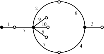
Figure 4: Realization of ${\rm S}_{5}$ acting on 10 edges of a bicolored plane map.

Riemann’s existence theorem implies that for any bicolored plane map there exists a Belyi function $F(x)$ which is unique up to a composition with $x\mapsto\mu(x)$ where $\mu(x)$ is a linear fractional transformation. In particular, since for the map shown in Fig. 4 the permutations $g_{0}$, $g_{1}$, $g_{\infty}$ coincide with $\sigma$, $\alpha$, $\varphi$, this pictures “proves” that there exists a rational function $F(x)$ whose monodromy group is permutation equivalent to the action of ${\rm S}_{5}$ on 10 points discussed above. Our next goal is to find this function explicitly.

3.2 A system of equations for the coefficients of Belyi function, and its solutions

In the rest of this section we will compute a Belyi function which produces a map isomorphic to that of Fig. 4 as a preimage of the segment $[0,1]$. A reader not interested in the details of the computation may just take our word for it that the resulting function is the one given in (9), and pass directly to Sec. 4. We will provide not all the details but only a minimum allowing the reader to reproduce our results.

The black vertices of the map are the preimages of 0, or, in other words, they are roots of the rational function $F$ we are looking for. Furthermore, the vertex of degree 6 is a root of multiplicity 6, the vertex of degree 3 is a triple root, and the vertex of degree 1 is a simple root. The freedom of choosing a linear fractional transformation $\mu(x)$ allows us to put these three points to any three chosen positions. Let us put, for example, the vertex of degree 6 to $x=0$, the vertex of degree 3, to $x=1$, and the vertex of degree 1, to $x=-1$. Then, the numerator of $F$ will take the form $x^{6}(x-1)^{3}(x+1)$.

The permutation $\varphi$ corresponds to the monodromy above $\infty$, and it has two cycles of length 5. Therefore, the function in question must have two poles of degree 5, one pole inside each face of the map. Suppose these poles to be the roots of a quadratic polynomial $x^{2}+ax+b$. Then, the Belyi function in question takes the form

$$F(x)\,=\,K\cdot\frac{x^{6}(x-1)^{3}(x+1)}{(x^{2}+ax+b)^{5}}$$

where $K,a,b$ are constants that remain to be determined.

Here the reader may be surprised. We are looking not for an arbitrary Belyi function but for a Laurent polynomial, aren’t we? Then, would it not be a better idea to use the same liberty of choice of three parameters and to put one of the poles to $x=0$, and the other one, to $x=\infty$? The answer is no: such a choice would not be a good idea – at least at this stage of the computation. The reason is related to Galois theory and will be explained later, in Sec. 3.4.

The white vertices of our map are the preimages of 1, or, in other words, the roots of the function $F(x)-1$. There are three white vertices of degree 2; they correspond to double roots of $F(x)-1$. Computing the derivative of $F$ we get

$$F^{\prime}(x)\,=\,K\cdot\frac{x^{5}(x-1)^{2}\,p(x)}{(x^{2}+ax+b)^{6}}$$

where

$$p(x)\,=\,(5a+2)\,x^{3}+(2a+10b+4)\,x^{2}-(a-2b)\,x-6b\,.$$

It becomes clear that $p(x)$ is the cubic polynomial whose roots are the three white vertices of degree 2, so the numerator of $F(x)-1$ must have $p(x)^{2}$ as a factor. Note also that the leading coefficient of this numerator is $K-1$. Thus, we can now write down the hypothetical form of $F(x)-1$ which we temporarily denote by $H(x)$:

$$H(x)\,=\,\frac{K-1}{(5a+2)^{2}}\cdot\frac{p(x)^{2}\,q(x)}{(x^{2}+ax+b)^{5}}$$

where $q(x)$ is yet unknown polynomial of degree 4, with the leading coefficient 1, whose roots are the four white vertices of degree 1. Denote

$$q(x)\,=\,x^{4}+cx^{3}+dx^{2}+ex+f$$

and compute the derivative of $H(x)$.

The results of the subsequent computations become more and more cumbersome. Their main steps go as follows. First of all, $H(x)$ is nothing else but another representation of $F(x)-1$, so we must get in the end $F^{\prime}(x)=H^{\prime}(x)$. Therefore, after having computed $H^{\prime}(x)$ we ask Maple to factor the difference $F^{\prime}(x)-H^{\prime}(x)$, and we get an expression

$$F^{\prime}(x)-H^{\prime}(x)\,=\,{\rm Const}\cdot\frac{p(x)\,r(x)}{(x^{2}+ax+b)^{6}}$$

where $r(x)$ is a (very huge) polynomial of degree 7. The final action to do is to equate $r(x)$ to zero: this means that we extract its coefficients and equate all of them to zero. This gives us a system of algebraic equations on the unknown parameters $K,a,b,c,d,e,f$.

The solution of the system thus obtained using the Maple-7 package takes 14 seconds. It takes significantly more time to enter all the involved formulas and operations. And it takes even more time to find our way among the solutions since they are many and varied.

3.3 Finding our way among the solutions

3.3.1 Maps with the same set of vertex and face degrees

If we analyse carefully the above procedure of constructing a system of equations, we will see that the only information we have used about the map of Fig. 4 is the set of degrees of the black vertices, the white vertices, and the faces of this map. However, there exist not one but 7 maps having the degree partition of the black vertices equal to $(6,3,1)=6^{1}3^{1}1^{1}\vdash 10$, that of white vertices equal to $(2,2,2,1,1,1,1)=2^{3}1^{4}\vdash 10$, and that of the faces equal to $(5,5)=5^{2}\vdash 10$. These maps are shown in Fig. 5. Therefore, the above computation must produce Belyi functions for all of them.

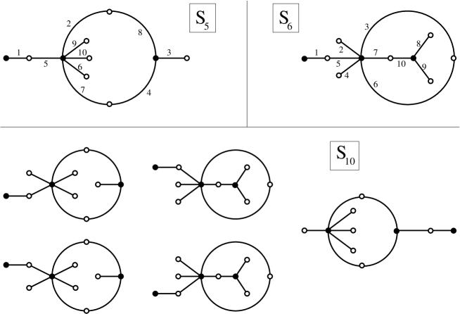
Figure 5: All the seven bicolored maps with the degree partition of the black vertices being $6^{1}3^{1}1^{1}$, that of the white vertices being $2^{3}1^{4}$, and that of the faces being $5^{2}$. Monodromy groups are also indicated.

The picture convinces us that these 7 maps do exist. In order to prove that there are no others we may compute the number of triples of permutations $(g_{0},g_{1},g_{\infty})$ of degree 10 having the same cycle structure as $(\sigma,\alpha,\varphi)$ and satisfying the equality $g_{0}g_{1}g_{\infty}=1$. For this end, we may use, for example, the following formula due to Frobenius:

Proposition 3.1.

Let $C_{1},C_{2},\ldots,C_{k}$ be conjugacy classes in a finite group $G$. Then the number ${\cal N}(G;C_{1},C_{2},\ldots,C_{k})$ of $k$-tuples $(x_{1},x_{2},\ldots,x_{k})$ of elements $x_{i}\in G$ such that each $x_{i}\in C_{i}$ and $x_{1}x_{2}\ldots x_{k}=1$, is equal to

$${\cal N}(G;C_{1},C_{2},\ldots,C_{k})\;=\;\frac{|C_{1}|\cdot|C_{2}|\cdot\ldots\cdot|C_{k}|}{|G|}\cdot\sum_{\chi}\frac{\chi(C_{1})\chi(C_{2})\ldots\chi(C_{k})}{({\rm dim\,}\chi)^{k-2}}\,,$$

where the sum is taken over the set of all irreducible characters of the group $G$.

Applying this formula to the group $G={\rm S}_{10}$, $k=3$, and the conjugacy classes $C_{1}$, $C_{2}$, $C_{3}$ determined by the cycle structures $6^{1}3^{1}1^{1}$, $2^{2}1^{4}$, and $5^{2}$, respectively, and computing the irreducible characters of ${\rm S}_{10}$ using the Maple package combinat, we get

$${\cal N}(G;C_{1},C_{2},C_{3})\;=\;25\,401\,600\;=\;7\cdot 10!\,.$$

None of the maps shown in Fig. 5 has a non-trivial orientation preserving automorphism; therefore, each of them admits $10!$ different labelings.

It is useful to determine monodromy groups of the functions corresponding to the above maps. For the map in the upper left corner we know already that, by construction, it is isomorphic to ${\rm S}_{5}$. For the 5 maps shown in the lower part of the figure, the order of the group (which can be calculated by the Maple package group, function grouporder) is equal to $10!$, and therefore the group is ${\rm S}_{10}$ itself. Finally, for the map in the upper right corner, using the same Maple package, or GAP, or the catalogue [9], we may establish that it is isomorphic to ${\rm S}_{6}$.

3.3.2 Galois action on maps and finding $F(x)$

We find the coefficients of the Belyi functions by solving a system of algebraic equations. Therefore, there is no wonder that these coefficients are algebraic numbers. The group of automorphisms of the field $\overline{{\mathbb{Q}}}$ of algebraic numbers is called the absolute Galois group and is denoted by $\Gamma={\rm Gal}(\overline{{\mathbb{Q}}}|{\mathbb{Q}})$. An element of the group $\Gamma$, acting simultaneously on all the coefficients of a given Belyi function, transforms it into another Belyi function which may correspond to another map.

Thus, bicolored maps split into the orbits of the above Galois action. The set of degrees of black and white vertices and faces is an invariant of this action; therefore, all the orbits are finite. Another invariant is the monodromy group. Looking once again at Fig. 5 we see that the set of 7 maps represented there splits into at least three Galois orbits: two orbits contain each a single element, while the set of the remaining 5 elements may constitute one orbit or further split into two or more orbits. The general theory suggests that for the singletons the coefficients of the corresponding Belyi functions must be rational numbers. And indeed, among our solutions we find two such functions:

$$F_{1}(x)\,=\,\frac{50000}{27}\cdot\frac{x^{6}(x-1)^{3}(x+1)}{(x^{2}+4x-1)^{5}}$$

and

$$F_{2}(x)\,=\,337500\cdot\frac{x^{6}(x-1)^{3}(x+1)}{(11x^{2}+4x-16)^{5}}\,.$$

At this stage we simply ask Maple to draw the $F$-preimages of the segment $[0,1]$ and find out that the function we are looking for is $F_{1}$: just compare Fig. 6 with Fig. 4. It is pictures like that in Fig. 6, obtained as Belyi preimages of the segment $[0,1]$, which are usually called dessins d’enfants.

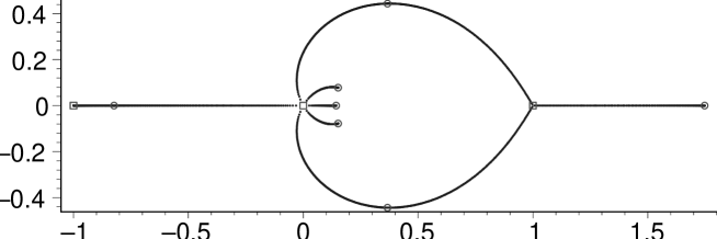
Figure 6: A Maple plot of the “dessin d’enfant” corresponding to the Belyi function $F_{1}$. Black vertices are marked by little squares.

The five remaining maps constitute an orbit of degree 5 defined over the splitting field of the polynomial

$$Q(t)\,=\,85237\,t^{5}-95206\,t^{4}+48850\,t^{3}-7456\,t^{2}+1606\,t-226\,.$$

This means that the coefficients of a Belyi function $F(x)$ are expressed in terms of (more exactly, as polynomials of degree $\leq 4$ in) a root of this polynomial. Taking one by one five roots we obtain five different Belyi functions which correspond to the five maps with the monodromy group ${\rm S}_{10}$ shown in the lower part of Fig. 5.

Notice that besides the solutions mentioned above, our system of algebraic equations produces a bunch of the so-called “parasitic solutions” representing various kinds of degeneracies. Some of them are easy to eliminate, others are not. For example, in one of the solutions we get $a=0$, $b=0$, which means that the denominator of $F$ is $x^{10}$, while its numerator contains $x^{6}$. This solution does correspond to a Belyi function, but of degree 4 instead of 10. Another easy case is $K=1$, $a=-2/5$, which leads to a division of zero by zero in the constant factor $(K-1)/(5a+2)^{2}$ of the function $H$ in Sec. 3.2. More difficult cases of degeneracies also exist but we will not go here into further details, as well as into many other subtleties proper to any experimental work. The questions already discussed show quite well why the computation of Belyi functions remains a handicraft instead of being an industry.

3.4 From a rational function to a Laurent polynomial

Now we may return to the question asked in Sec. 3.2 and explain why we decided to compute a “generic” Belyi function instead of looking from the very beginning for a Laurent polynomial.

We see that, while $F_{1}$ is defined over ${\mathbb{Q}}$, its two poles are not: they are roots of the quadratic polynomial $x^{2}+4x-1$; concretely, they are equal to $-2\pm\sqrt{5}$. Any linear fractional transformation of the variable $x$ sending one of theses poles to 0 and the other one to $\infty$ would inevitably add $\sqrt{5}$ to the field to which belong the coefficients of Belyi functions. Thus, the functions defined over ${\mathbb{Q}}$ would become defined over ${\mathbb{Q}}(\sqrt{5})$, the orbit of degree 5 would become one of degree 10 (with each of the five maps being represented twice), parasitic solutions would also become more cumbersome (and their parasitic nature would be more difficult to detect), and so on. And without doubt Maple would have a much harder work to solve the corresponding more complicated system of algebraic equations.

But from now on, after making all the above computations with the simplest possible fields, we can easily transform $F_{1}$ into a Laurent polynomial. The transformation

$$z\,=\,\frac{(2-\sqrt{5})x-1}{(2+\sqrt{5})x-1}$$

sends the pole $-2-\sqrt{5}$ to 0 and $-2+\sqrt{5}$ to $\infty$, and also sends 0 to 1. Substituting into $F_{1}(x)$ its inverse

$$x\,=\,\frac{z-1}{(2+\sqrt{5})z-(2-\sqrt{5})}$$

we obtain the Laurent polynomial of Theorem 1.1:

$$L(z)\,=\,K\cdot\frac{(z-1)^{6}(z-a)^{3}(z-b)}{z^{5}}$$

where

$$K=\frac{11+5\sqrt{5}}{216},\qquad a=\frac{-3+\sqrt{5}}{2},\qquad b=\frac{7-3\sqrt{5}}{2}\,.$$

4 Proof of the main theorem

We are looking for Laurent polynomials $Q_{j}$, $0\leq j\leq 4$, of the form

$$Q_{j}(z)\,=\,\sum_{k=-j}^{j}s_{k}z^{k}$$ (10)

(we set $Q_{0}=1$) satisfying the equation (8). However, it is clear that we may multiply $Q_{j}$ by a constant, and also add to $Q_{j}$ an arbitrary linear combination of $Q_{i}$ for $i<j$, and this gives us another solution having the same form. Therefore, in order to achieve uniqueness, we impose on $Q_{j}$ the following three conditions:

1. The coefficient $s_{-j}$ is equal to one.

2. For $i=-j+1,\ldots,0$ the coefficients $s_{i}$ are equal to zero.

3. $\displaystyle\int_{S^{1}}{L}^{i}dQ_{j}=0$    for all    $1\leq i\leq j$ .

The Laurent polynomial $Q_{j}$ has $2j+1$ coefficients; the first two conditions fix $j+1$ of them, while the third condition provides us with $j$ additional linear equations on coefficients. In order to ensure that the integrals in the third condition vanish, according to the Cauchy theorem, we must calculate the coefficients preceding $z^{-1}$ in $L^{i}\cdot Q^{\prime}_{j}$, $1\leq j\leq 4$, $1\leq i\leq j$, and set them to zero. The existence and uniqueness of solutions will be explained later (in Step 3 of the proof). The results of the calculation are collected below.

$$Q_{0}\,=\,1\,,$$

$$Q_{1}\,=\,{\frac{{z}^{2}+1}{z}}\,,$$

$$Q_{2}\,=\,{\frac{-(9+4\,\sqrt{5})\,z^{4}+(20+8\,\sqrt{5})\,z^{3}+1}{{z}^{2}}}\,,$$

$$Q_{3}\,=\,\frac{\left(\frac{47}{2}+\frac{21}{2}\,\sqrt{5}\right)z^{6}-\left(\frac{195}{2}+\frac{87}{2}\,\sqrt{5}\right)z^{5}+\left(\frac{255}{2}+\frac{111}{2}\,\sqrt{5}\right)z^{4}\,+\,1}{z^{3}}\,,$$

$$Q_{4}=\frac{-(9+4\,\sqrt{5})\,z^{8}+(130+58\,\sqrt{5})\,z^{7}-(630+282\,\sqrt{5})\,z^{6}+(910+406\,\sqrt{5})\,z^{5}+1}{z^{4}}.$$

Now, everything is ready in order to prove the main theorem. The proof is divided into several steps.

Step 1.

First of all, we must check that the Laurent polynomials $Q_{j}$, $1\leq j\leq 4$, satisfy the equalities

$$\int_{S^{1}}{L}^{i}{d\,}Q\,=\,0$$ (11)

for all $i\geq 0$ (for $Q_{0}$ it is obvious). For this purpose we may use Theorem 7.1 of [19] and verify this equality only for a finite number of $i$, namely, for

$$1\,\leq\,i\,\leq\,(N-1)\cdot{\rm deg\,}Q+1,$$ (12)

where $N$ is the size of the orbit of the vector

$$(1,1,1,1,1,-1,-1,-1,-1,-1)$$

under the action of the monodromy group of $L$. In our case, ${\rm deg\,}Q_{j}=2j$, $1\leq j\leq 4,$ and $N=12$; therefore, the maximal value of the right hand side of (12) is equal to 89. The verification for all the four polynomials $Q_{j}$ takes less than one minute of work of Maple-11.

Step 2.

Observe that if a Laurent polynomial $Q$ is a solution of (11) then for any polynomial $R$ the Laurent polynomial $\widehat{Q}=R(L)\cdot Q$ is also a solution of (11). Indeed, it is enough to prove it for $R=z^{k}$, $k\geq 1$. We have:

$$\int_{S_{1}}L^{i}{d\,}(L^{k}Q)\,=\,\int_{S_{1}}L^{i+k}{d\,}Q+\int_{S_{1}}L^{i}Q\,{d\,}L^{k}\,.$$

The first integral in the right-hand side of this equality vanishes by (11). On the other hand, for the second integral we have:

$$\int_{S^{1}}L^{i}Q{d\,}L^{k}=k\int_{S^{1}}L^{i+k-1}Q{d\,}L=\frac{k}{i+k}\int_{S^{1}}Q{d\,}L^{k+i}=-\frac{k}{i+k}\int_{S^{1}}L^{k+i}{d\,}Q\,,$$

and therefore this integral also vanishes.

Step 3.

The final ingredient we need is Theorem 6.7 of [19] which states that if the leading degree of a Laurent polynomial $L$ is a prime number $p$ (in our case $p=5$), and if $Q$ is a polynomial (that is, a common one, not a Laurent polynomial) such that (11) holds, then either $L(z)=L_{1}(z^{p})$ for some Laurent polynomial $L_{1}$ while $Q$ is a linear combination of the monomials $z^{i}$ with $i$ not being multiples of $p$, or $Q$ is a constant. Since the Laurent polynomial $L$ we are working with is not of the form $L(z)=L_{1}(z^{p})$ this result implies that a polynomial $Q$ cannot satisfy (11) unless $Q$ is a constant.

This fact also explains the uniqueness of $Q_{j}$. Indeed, if $Q_{j}^{(1)}$ and $Q_{j}^{(2)}$ are two solutions of the equations imposed on $Q_{j}$ at the beginning of this section, then their difference $Q_{j}^{(1)}-Q_{j}^{(2)}$ is also a solution of the Laurent polynomial moment problem. But this difference is a polynomial (since the terms $z^{-j}$ in $Q_{j}^{(1)}$ and $Q_{j}^{(2)}$ cancel) and therefore must reduce to its constant term; but the constant term of this polynomial is equal to zero.

The uniqueness of the solution implies the non-degeneracy of the matrix of the system, and the non-degeneracy, in its turn, implies existence.

Step 4.

Now, let us suppose that $Q$ is a Laurent polynomial satisfying (11) and $m(Q)\leq 0$ is the minimal degree of a monomial in $Q$. Let $m(Q)=-5k_{0}-j_{0}$, where $0\leq j_{0}\leq 4$ and $k_{0}\geq 0$. Then for any $c_{0}\in{\mathbb{C}}$ the Laurent polynomial

$$Q^{(1)}\,=\,Q-c_{0}\,L^{k_{0}}\cdot Q_{j_{0}}\,,$$

is a solution (11). Furthermore, choosing an appropriate $c_{0}$ we can assume that $m(Q^{(1)})>m(Q)$ (here we use the fact that the coefficient $s_{-j}$ in $Q_{j}$ is not zero). Now, if $m(Q^{(1)})=-5k_{1}-j_{1}$, where $0\leq j_{1}\leq 4$ and $k_{1}\geq 0$, then, setting

$$Q^{(2)}\,=\,Q^{(1)}-c_{1}\,L^{k_{1}}\cdot Q_{j_{1}}$$

for an appropriate $c_{1}$ we obtain a solution (11) with $m(Q^{(2)})>m(Q^{(1)})$. Continuing in this way we will eventually arrive to a solution $Q^{(r)}$ of (11) for which $m(Q^{(r)})\geq 0$. In view of the result cited in Step 3 such a solution should be a constant $c\in{\mathbb{C}}$. Therefore,

$$Q\,=\,c\,+\,\sum_{i=0}^{r-1}c_{i}\,L^{k_{i}}\cdot Q_{j_{i}}\,=\,\sum_{j=0}^{4}(R_{j}\circ L)\cdot Q_{j}$$

for some polynomials $R_{0},R_{1},R_{2},R_{3},R_{4}$. The theorem is proved.

Final remarks.

In general, it is not known if the reducibility of the action of the monodromy group $G_{L}$ of a Laurent polynomial $L$ of degree $n$ on the space ${\mathbb{Q}}^{n}$ always implies a non-trivial structure of solutions of the corresponding moment problem. The only facts which follow from the general theory are as follows:

• The reducibility of the above action implies the existence of a rational function $Q$, which is not a rational function in $L$, such that the generating function for the sequence of the moments

  $$m_{i}=\int_{S^{1}}L^{i}\,dQ,\ \ \ i\geq 0,$$

  is rational (see Sec. 8.3 of [19]).

• If the above function $Q$ turns out to be a Laurent polynomial, then the rationality of the generating function implies its vanishing (see Theorem 3.4 of [19]).

It would be interesting to understand in a more profound way what is the underlying mechanism which relates the structure of solutions of the moment problem for $L$ with the structure of the representation of $G_{L}$.

References

- [1] M. Blinov, M. Briskin, Y. Yomdin, Local center conditions for a polynomial Abel equation and cyclicity of its zero solution, in “Complex analysis and dynamical systems II”, Contemp. Math., vol. 382, AMS, Providence, RI, 65–82 (2005).
- [2] M. Briskin, J.-P. Françoise, Y. Yomdin, Une approche au problème du centre-foyer de Poincaré, C. R. Acad. Sci. Paris, Sér. I, Math., vol. 326, no. 11, 1295–1298 (1998).
- [3] M. Briskin, J.-P. Françoise, Y. Yomdin, Center conditions, compositions of polynomials and moments on algebraic curve, Ergodic Theory Dyn. Syst., vol. 19, no. 5, 1201–1220 (1999).
- [4] M. Briskin, J.-P. Françoise, Y. Yomdin, Center condition II: Parametric and model center problems, Israel J. Math., vol. 118, 61–82 (2000).
- [5] M. Briskin, J.-P. Françoise, Y. Yomdin, Center condition III: Parametric and model center problems, Israel J. Math., vol. 118, 83–108 (2000).
- [6] M. Briskin, J.-P. Françoise, Y. Yomdin, Generalized moments, center-focus conditions and compositions of polynomials, in “Operator Theory, System Theory and Related Topics”, Oper. Theory Adv. Appl., vol. 123, 161–185 (2001).
- [7] M. Briskin, N. Roytvarf, Y. Yomdin, Center conditions at infinity for Abel differential equations, to appear in Annals of Mathematics, available at http://annals.math.princeton.edu/issues/AcceptedPapers.html
- [8] M. Briskin, Y. Yomdin, Tangential version of Hilbert 16th problem for the Abel equation, Moscow Math. J., vol. 5, no. 1, 23–53 (2005).
- [9] G. Butler, J. McKay, The transitive groups of degree up to eleven, Comm. in Algebra, vol. 8, no. 11, 863–911 (1983).
- [10] C. Christopher, Abel equations: composition conjectures and the model problem, Bull. Lond. Math. Soc., vol. 32, no. 3, 332–338 (2000).
- [11] K. Girstmair, Linear dependence of zeros of polynomials and construction of primitive elements, Manuscripta Math., vol. 39, no. 1, 81–97 (1982).
- [12] S. K. Lando, A. K. Zvonkin, Graphs on Surfaces and Their Applications, Encyclopaedia of Mathematical Sciences, vol. 141 (II), Berlin, Springer-Verlag (2004).
- [13] F. Pakovich, M. Muzychuk, Solution of the polynomial moment problem, arXiv:0710.4085. To appear in Proc. London Math. Soc. (2009).
- [14] F. Pakovich, A counterexample to the “composition conjecture”, Proc. Amer. Math. Soc., vol. 130, no. 12, 3747–3749 (2002).
- [15] F. Pakovich, On the polynomial moment problem, Math. Research Letters, vol. 10, 401–410 (2003).
- [16] F. Pakovich, Polynomial moment problem, Addendum to the paper [23].
- [17] F. Pakovich, On polynomials orthogonal to all powers of a Chebyshev polynomial on a segment, Israel J. Math, vol. 142, 273–283 (2004).
- [18] F. Pakovich, On polynomials orthogonal to all powers of a given polynomial on a segment, Bull. Sci. Math., vol. 129, no. 9, 749–774 (2005).
- [19] F. Pakovich, On rational functions orthogonal to all powers of a given rational function on a curve, preprint, arXiv:0910.2105v1.
- [20] F. Pakovich, Generalized “second Ritt theorem” and explicit solution of the polynomial moment problem, preprint, arXiv:0908.2508v2.
- [21] F. Pakovich, N. Roytvarf, Y. Yomdin, Cauchy type integrals of algebraic functions, Israel J. Math., vol. 144, 221–291 (2004).
- [22] N. Roytvarf, Generalized moments, composition of polynomials and Bernstein classes, in “Entire Functions in Modern Analysis: B. Ya. Levin Memorial Volume”, Israel Math. Conf. Proc., vol. 15, 339–355 (2001).
- [23] Y. Yomdin, Center problem for Abel equation, compositions of functions and moment conditions, Moscow Math. J., vol. 3, no. 3, 1167–1195 (2003).