The calculation of nucleon strangeness form factors from $N_{f}=2+1$ clover fermion lattice QCD

Abstract:

We study the strangeness electromagnetic form factors of the nucleon from the $N_{f}=2+1$ clover fermion lattice QCD calculation. The disconnected insertions are evaluated using the Z(4) stochastic method, along with unbiased subtractions from the hopping parameter expansion. In addition to increasing the number of Z(4) noises, we find that increasing the number of nucleon sources for each configuration improves the signal significantly. We obtain $G_{M}^{s}(0)=-0.017(25)(07)$, where the first error is statistical, and the second is the uncertainties in $Q^{2}$ and chiral extrapolations. This is consistent with experimental values, and has an order of magnitude smaller error. We also study the strangeness second moment of the partion distribution function of the nucleon, $\langle x^{2}\rangle_{s-\bar{s}}$.

1 Introduction

In the pursuit of the full understanding of QCD, it has been essential to study the structure of the nucleon. The strangeness content of the nucleon particularly attracts a great interest lately. As the lightest non-valence quark structure, it is an ideal probe for the virtual sea quarks in the nucleon. Recently, intensive experiments have been carried out for the electromagnetic form factors by SAMPLE, A4, HAPPEX, G0, through parity-violating electron scattering (PVES). The global analyses [1, 2, 3] have produced, e.g., $G_{E}^{s}(Q^{2})=-0.008(16)$ and $G_{M}^{s}(Q^{2})=0.29(21)$ at $Q^{2}=0.1{\rm GeV}^{2}$ [2], but substantial errors still exist so that the results are consistent with zero. Making tighter constraints on these form factors from the theoretical side is one of the challenges in QCD calculation. Moreover, such constraints, together with experimental inputs, can lead to more precise determinations of various interesting quantities, such as the axial form factor $G_{A}^{s}$ [3], and the electroweak radiative corrections including the nucleon anapole moment, $\tilde{G}_{A}$ [1, 4]. Unfortunately, the theoretical status of strangeness form factors remains quite uncertain. For instance, the values for the magnetic moment $G_{M}^{s}(0)$ from different model calculations vary widely, from $-0.5$ to $+0.1$. One may put an expectation on lattice simulation as the most desirable first-principle calculation. The evaluation of strangeness matrix elements, however, has been a serious challenge to the lattice QCD, since it requires the disconnected insertion (DI), for which the straightforward calculation requires all-to-all propagators and is prohibitively expensive. Consequently, there have been only few DI calculations, where the all-to-all propagators are stochastically estimated, and quenched approximation is used with Wilson fermion  [5, 6, 7]. There are also several indirect estimates using quenched [8, 9] or unquenched [10] lattice data for the connected insertion (CI) part, and the experimental magnetic moments (or electric charge radii) for octet baryons as inputs. In this proceeding, we present the first full QCD lattice simulation of the direct DI calculation for strangeness form factors. For details of this study, see Ref. [11].

We also study the strangeness contribution to the lowest moments of the parton distribution function of the nucleon, $\langle x\rangle$, $\langle x^{2}\rangle$ [12]. In particular, the strangeness second moment $\langle x^{2}\rangle_{s-\bar{s}}=\int dxx^{2}(s(x)-\bar{s}(x))$ is important quantity in relation to the NuTeV anomaly. The NuTeV experiments [13] measured the Weinberg angle, which is 3 $\sigma$ away from the world average value. While this may indicate the existence of New Physics, it is necessary to make exhaustive investigations on hidden systematic uncertainties before making such a conclusion. In fact, the asymmetry between strange and anti-strange parton distribution is one of the probable candidates to explain the NuTeV anomaly without New Physics. We note that lattice QCD can make a great contribution to this issue, by measuring the strangeness asymmetry in the second moment, which provides essential constraint to the asymmetry in the strangeness parton distribution function. In this proceeding, we present a preliminary result of $\langle x^{2}\rangle_{s-\bar{s}}$ as the first full QCD calculation for this quantity.

2 Formalism and lattice calculation parameters

We employ $N_{f}=2+1$ dynamical configurations with nonperturbatively ${\cal O}(a)$ improved clover fermion and RG-improved gauge action generated by CP-PACS/JLQCD Collaborations [14]. We use $\beta=1.83$ and $c_{sw}=1.7610$ configurations with the lattice size of $L^{3}\times T=16^{3}\times 32$. The lattice spacing was determined as $a^{-1}=1.625{\rm GeV}$, using $K$-input or $\phi$-input [14]. For the hopping parameters of $u$,$d$ quarks ($\kappa_{ud}$) and $s$ quark ($\kappa_{s}$), we use $\kappa_{ud}=$ $0.13825$, $0.13800$, and $0.13760$, which correspond to $m_{\pi}=$ $0.60$, $0.70$, and $0.84$ ${\rm GeV}$, respectively, and $\kappa_{s}=0.13760$ is fixed. We perform the calculation only at the dynamical quark mass points, where 800 configurations are used for $\kappa_{ud}=$ $0.13760$, and 810 configurations for $\kappa_{ud}=$ $0.13800$, $0.13825$. The periodic boundary condition is imposed in all space-time directions for the valence quarks.

We calculate the two point function (2pt) $\Pi^{\rm 2pt}$ and three point function (3pt) $\Pi^{\rm 3pt}_{J_{\mu}}$,

$$\Pi^{\rm 3pt}_{J_{\mu}}(\vec{p},t_{2};\ \vec{q},t_{1};\ \vec{p^{\prime}}=\vec{p}-\vec{q},t_{0})$$ (1)

$$= \sum_{\vec{x_{2}},\vec{x_{1}}}e^{-i\vec{p}\cdot(\vec{x}_{2}-\vec{x}_{0})}\times e^{+i\vec{q}\cdot(\vec{x}_{1}-\vec{x}_{0})}\langle 0|{\rm T}\left[\chi_{N}(\vec{x}_{2},t_{2}){J_{\mu}}(\vec{x}_{1},t_{1})\bar{\chi}_{N}(\vec{x}_{0},t_{0})\right]|0\rangle,$$

where $\chi_{N}$ is the nucleon interpolation field and the insertion $J_{\mu}$ is given by the point-split conserved current $J_{\mu}(x+\mu/2)=(1/2)\times$ $\left[\bar{s}(x+\mu)(1+\gamma_{\mu})U_{\mu}^{\dagger}(x)s(x)-\bar{s}(x)(1-\gamma_{\mu})U_{\mu}(x)s(x+\mu)\right].$

Electromagnetic form factors can be obtained using $\vec{p}=\vec{0}$, $\vec{p^{\prime}}=-\vec{q}$ kinematics for the forward propagation ($t_{2}\gg t_{1}\gg t_{0}$) [5]. In this work, we consider the backward propagation ($t_{2}\ll t_{1}\ll t_{0}$) as well, in order to increase statistics. The formulas for $G_{E}^{s}$ and $G_{M}^{s}$ are summarized as

$$R_{\mu}^{\pm}(\Gamma_{\rm pol}^{\pm}) \equiv \frac{{\rm Tr}\left[\Gamma_{\rm pol}^{\pm}\cdot\Pi^{\rm 3pt}_{J_{\mu}}(\vec{0},{t}_{2};\ \pm\vec{q},{t}_{1};\ -\vec{q},t_{0})\right]}{{\rm Tr}\left[\Gamma_{e}^{\pm}\cdot\Pi^{\rm 2pt}(\pm\vec{q},t_{1};\ t_{0})\right]}\times\frac{{\rm Tr}\left[\Gamma_{e}^{\pm}\cdot\Pi^{\rm 2pt}(\vec{0},t_{1};\ t_{0})\right]}{{\rm Tr}\left[\Gamma_{e}^{\pm}\cdot\Pi^{\rm 2pt}(\vec{0},t_{2};\ t_{0})\right]},$$ (2)

$$R_{\mu=4}^{\pm}(\Gamma_{\rm pol}^{\pm}=\Gamma_{e}^{\pm}) = \pm G_{E}^{s}(Q^{2}),\qquad R_{\mu=i}^{\pm}(\Gamma_{\rm pol}^{\pm}=\Gamma_{k}^{\pm})=\frac{\mp\epsilon_{ijk}q_{j}}{E^{q}_{N}+m_{N}}G_{M}^{s}(Q^{2}),$$ (3)

where $\{i,j,k\}\neq 4$, $\Gamma_{e}^{\pm}\equiv(1\pm\gamma_{4})/2$ , $\Gamma_{k}^{\pm}\equiv(\pm i)/2\times(1\pm\gamma_{4})\gamma_{5}\gamma_{k}$ and $E^{q}_{N}\equiv\sqrt{m_{N}^{2}+\vec{q}^{\,2}}$. The upper (lower) sign corresponds to the forward (backward) propagation. Furthermore, we consider another kinematics of $\vec{p}=\vec{q}$, $\vec{p^{\prime}}=\vec{0}$, where the analogs of Eqs. (2), (3) hold. We find that the results from the latter kinematics have similar size of statistical errors as those from the former, and the average of them yields better results. Hereafter, we present results from total average of two kinematics and forward/backward propagations, unless otherwise noted. In order to extract the matrix elements, we take the summation over the insertion time $t_{1}$, symbolically given as $R^{t}_{E,M}\equiv\frac{1}{K_{E,M}^{\pm}}\sum_{t_{1}=t_{0}+t_{s}}^{t_{2}-t_{s}}R^{\pm}_{\mu}={\rm const.}+t_{2}\times G_{E,M}^{s},$ where $K_{E,M}^{\pm}$ are trivial kinematic factors appearing in Eq. (3) and $t_{s}$ is chosen so that the error is minimal. We thus obtain $G_{E,M}^{s}$ as the linear slope of $R^{t}_{E,M}$ against $t_{2}$.

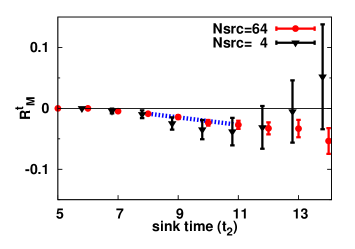
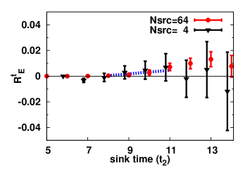
Figure 1: $R_{M}^{t}$ (left) and $R_{E}^{t}$ (right) with $\kappa_{ud}=0.13760$, $\vec{q}^{\,2}=2\cdot(2\pi/La)^{2}$, $N_{src}=64$ (circles) and $N_{src}=4$ (triangles, with offset for visibility), plotted against the nucleon sink time $t_{2}$. The dashed line is the linear fit where the slope corresponds to the form factor.

The calculations of 3pt need the evaluation of DI. We use the stochastic method [15], with Z(4) noises in color, spin and space-time indices. We generate independent noises for different configurations, in order to avoid possible auto-correlation. To reduce fluctuations, we use the charge conjugation and $\gamma_{5}$-hermiticity (CH), and parity symmetry [11, 16, 17]. We also perform unbiased subtractions [18] to reduce the off-diagonal contaminations to the variance. For subtraction operators, we employ those obtained from hopping parameter expansion (HPE) for the propagator $M^{-1}$, $\frac{1}{2\kappa}M^{-1}=\frac{1}{1+C}+\frac{1}{1+C}(\kappa D)\frac{1}{1+C}+\cdots$ where $D$ denotes the Wilson-Dirac operator and $C$ the clover term. We subtract up to order $(\kappa D)^{4}$ term, and the statistical error is reduced by a factor of 2.

In the stochastic method, it is quite expensive to achieve a good signal to noise ratio (S/N) just by increasing $N_{noise}$ because S/N improves with $\sqrt{N_{noise}}$. In view of this, we use many nucleon point sources $N_{src}$ in the evaluation of the 2pt part for each configuration [17]. Since the calculations of the loop part and 2pt part are independent of each other, this is expected to be an efficient way. In particular, for the $N_{noise}\gg N_{src}$ case, we observe that S/N improves almost ideally, by a factor of $\sqrt{N_{src}}$. We take $N_{src}=64$ for $\kappa_{ud}=0.13760$ and $N_{src}=82$ for $\kappa_{ud}=0.13800,0.13825$, where locations of sources are taken so that they are separated in 4D-volume as much as possible.

3 Results for strangeness form factors

We calculate for the five smallest momentum-squared points, $\vec{q}^{\,2}=n\cdot(2\pi/La)^{2}\$ $(n=0$–$4)$. Typical figures for $R^{t}_{E,M}$ are shown in Fig. 1. One can observe the significant S/N improvement by increasing $N_{src}$. Of particular interest is that, for all $\kappa_{ud}$ simulations, $G_{M}^{s}(Q^{2})$ is found to be negative with 2-3 $\sigma$ signals for low $Q^{2}$ regions. In order to determine the magnetic moment, the $Q^{2}$ dependence of $G_{M}^{s}(Q^{2})$ is studied. We employ the dipole form in the $Q^{2}$ fit, $G_{M}^{s}(Q^{2})=G_{M}^{s}(0)/(1+Q^{2}/\Lambda^{2})^{2}$, where reasonable agreement with lattice data is observed. For the electric form factor, we employ $G_{E}^{s}(Q^{2})=g_{E}^{s}\cdot Q^{2}/(1+Q^{2}/\Lambda^{2})^{2}$, considering that $G_{E}^{s}(0)=0$ from the vector current conservation. In the practical fit of $G_{E}^{s}(Q^{2})$, however, reliable extraction of the pole mass $\Lambda$ is impossible because $G_{E}^{s}(Q^{2})$ data are almost zero within error. Therefore, we assume that $G_{E}^{s}(Q^{2})$ has the same pole mass as $G_{M}^{s}(Q^{2})$, and perform a one-parameter fit for $g_{E}^{s}$ [11].

Finally, we perform the chiral extrapolation for the fitted parameters. Since our quark masses are relatively heavy, we consider only the leading dependence on $m_{K}$, which is obtained by heavy baryon chiral perturbation theory (HB$\chi$PT). For the magnetic moment $G_{M}^{s}(0)$, we fit linearly in terms of $m_{K}$ [5, 19]. For the pole mass $\Lambda$, we take that the magnetic mean-square radius $\langle r^{2}_{s}\rangle_{M}=12G_{M}^{s}(0)/\Lambda^{2}$ behaves as $1/m_{K}$ [19]. For $g_{E}^{s}$, we use the electric radius $\langle r^{2}_{s}\rangle_{E}=-6g_{E}^{s}$ which has an $\ln(m_{K}/\mu)$ behavior [19], and we take the scale $\mu=1$ GeV. The chiral extrapolated results are $G_{M}^{s}(0)=-0.017(25)$, $\Lambda a=0.58(16)$, $\langle r_{s}^{2}\rangle_{M}=-7.4(71)\times 10^{-3}{\rm fm}^{2}$, $\langle r_{s}^{2}\rangle_{E}=-2.4(15)\times 10^{-3}{\rm fm}^{2}$.

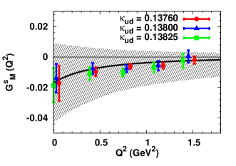
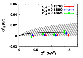
Figure 2: The chiral extrapolated results for $G_{M}^{s}(Q^{2})$ (left) and $G_{E}^{s}(Q^{2})$ (right) plotted with solid lines. Shaded regions represent the error-band with statistical and systematic error added in quadrature. Shown together are the lattice data (and $Q^{2}$-extrapolated $G_{M}^{s}(0)$) for $\kappa_{ud}=$ 0.13760 (circles), 0.13800 (triangles), 0.13825 (squares) with offset for visibility.

Before quoting the final results, we consider the systematic uncertainties yet to be addressed. First, we analyze the ambiguity of $Q^{2}$ dependence in form factors, by employing the monopole form [11]. The results are found to be consistent with those from the dipole fit, and we take the difference as systematic uncertainties. Second, we study the uncertainties in chiral extrapolation by testing two alternative extrapolations. In the first one, we take into account the nucleon mass dependence on the quark mass, using the lattice nucleon mass. From the physical viewpoint, this corresponds to measuring the magnetic moment not in units of lattice magneton but physical magneton [20]. In the second alternative, we use the linear fit in terms of $m_{K}^{2}$, observing the results have weak quark mass dependence. In either of alternative analyses, we find that the results are consistent with previous ones. While a further clarification with physically light quark mass simulation and a check on convergence of HB$\chi$PT [21] is desirable, we use the dependence of results on different extrapolations as systematic uncertainties. Third, we examine the contamination from excited states. Because our spectroscopy study indicates that the mass of Roper resonance is massive compared to the $S_{11}$ state on the current lattice [22], the dominant contaminations are (transition) form factors associated with $S_{11}$. On this point, we find that such contaminations can be eliminated theoretically, making the appropriate substitutions for $\Gamma_{e}^{\pm}$ in Eq. (2) and $\{\Gamma_{e}^{\pm},\ \Gamma_{k}^{\pm}\}$ in Eq. (3) [11]. It is found that the results from this formulation are basically the same as before, so we conclude that the contamination regarding the $S_{11}$ state is negligible.

As remaining sources of systematic error, one might worry that the finite volume artifact could be substantial considering that the spacial size of the lattice is about $(2{\rm fm})^{3}$. However, we recall that Sachs radii are found to be quite small, $|\langle r_{s}^{2}\rangle_{E,M}|\ll 0.1{\rm fm}^{2}$, which indicates a small finite volume artifact. For the discretization error, we conclude that finite $(qa)$ discretization error is negligible, since the lattice nucleon energy is found to be consistent with the dispersion relation. As another discretization error, we note that $m_{N}$ ($m_{K}$) is found to have 6 (8) % error for the current configurations [14, 23]. Considering the dependence of $G_{E,M}^{s}$ on these masses, we estimate that the discretization errors amount to $\mathrel{\mathchoice{\lower 2.58334pt\vbox{\halign{$\m@th\displaystyle\hfill#\hfil$\cr<\crcr\sim\crcr}}}{\lower 2.58334pt\vbox{\halign{$\m@th\textstyle\hfill#\hfil$\cr<\crcr\sim\crcr}}}{\lower 2.58334pt\vbox{\halign{$\m@th\scriptstyle\hfill#\hfil$\cr<\crcr\sim\crcr}}}{\lower 2.58334pt\vbox{\halign{$\m@th\scriptscriptstyle\hfill#\hfil$\cr<\crcr\sim\crcr}}}}10$%, and are much smaller than the statistical errors. Of course, more quantitative investigations are desirable, and such work is in progress.

To summarize the results of form factors, we obtain $G_{M}^{s}(0)=-0.017(25)(07)$, where the first error is statistical and the second is systematic from uncertainties of the $Q^{2}$ extrapolation and chiral extrapolation. We also obtain $\Lambda a=0.58(16)(19)$ for dipole mass or $\tilde{\Lambda}a=0.34(17)(11)$ for monopole mass, and $g_{E}^{s}=0.027(16)(08)$. These lead to $G_{M}^{s}(Q^{2})=-0.015(23)$, $G_{E}^{s}(Q^{2})=0.0022(19)$ at $Q^{2}=0.1{\rm GeV}^{2}$, where error is obtained by quadrature from statistical and systematic errors. We also obtained, e.g., $G_{M}^{s}(Q^{2})=-0.014(21)$, $G_{E}^{s}(Q^{2})=0.0041(38)$ at $Q^{2}=0.22{\rm GeV}^{2}$. Note that these are consistent with the world averaged data at $Q^{2}=0.1{\rm GeV}^{2}$ [1, 2, 3] and the recent measurement at Mainz [24], $G_{M}^{s}(Q^{2})=-0.14(11)(11)$, $G_{E}^{s}(Q^{2})=0.050(38)(19)$ at $Q^{2}=0.22{\rm GeV}^{2}$, with an order of magnitude smaller error. In Fig. 2, we plot our results for $G_{M}^{s}(Q^{2})$, $G_{E}^{s}(Q^{2})$, where the shaded regions correspond to the square-summed error.

4 Results for the strangeness second moment $\langle x^{2}\rangle_{s-\bar{s}}$

In the calculation of the strangeness second moment, $\langle x^{2}\rangle_{s-\bar{s}}$, we use the following three-index operator $T_{4ii}$ as the insertion operator in 3pt,

$$T_{4ii} \equiv -\frac{1}{3}\left[\bar{s}\gamma_{4}\overleftrightarrow{D}_{i}\overleftrightarrow{D}_{i}s+\bar{s}\gamma_{i}\overleftrightarrow{D}_{4}\overleftrightarrow{D}_{i}s+\bar{s}\gamma_{i}\overleftrightarrow{D}_{i}\overleftrightarrow{D}_{4}s\right]\qquad(i\neq 4).$$ (4)

Taking the kinematics of $\vec{p^{\prime}}=\vec{p}$, $\vec{q}=\vec{0}$, the following ratio of 3pt to 2pt corresponds to the second moment [17],

$$\frac{{\rm Tr}\left[\Gamma_{e}^{\pm}\cdot\Pi^{\rm 3pt}_{T_{4ii}}(\pm\vec{p},t_{2};\ \vec{0},t_{1};\ \pm\vec{p},t_{0})\right]}{{\rm Tr}\left[\Gamma_{e}^{\pm}\cdot\Pi^{\rm 2pt}(\pm\vec{p},t_{2};\ t_{0})\right]}=\pm p_{i}^{2}\cdot\langle x^{2}\rangle_{s-\bar{s}},$$ (5)

where the upper (lower) sign corresponds to the forward (backward) propagation as before.

In the evaluation of the DI, we can apply basically the same technique which is used in the calculation of the strange form factors. Because of the difference of the structure of the insertion operator, we perform the unbiased subtraction from HPE up to order $(\kappa D)^{3}$ term.

In Fig. 3 , we plot the ratio of 3pt to 2pt in terms of the nucleon sink time, $t_{2}$, where the linear slope corresponds to the signal of $\langle x^{2}\rangle_{s-\bar{s}}$. One can clearly observe that S/N improves significantly by increasing $N_{src}$, as was observed in the form factor study. Yet, the signal of $\langle x^{2}\rangle_{s-\bar{s}}$ in this figure is still consistent with zero. In order to obtain the final result, detailed analyses are in progress.

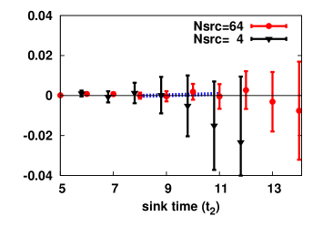
Figure 3: The ratio of 3pt to 2pt with $\kappa_{ud}=0.13760$, $\vec{p}^{\,2}=(2\pi/La)^{2}$, $N_{src}=64$ (circles) and $N_{src}=4$ (triangles, with offset for visibility), plotted against the nucleon sink time $t_{2}$. The dashed line is the linear fit where the slope corresponds to the second moment.

5 Summary

We have studied the strangeness electromagnetic form factors of the nucleon from the $N_{f}=2+1$ clover fermion lattice QCD calculation. It has been found that calculating many nucleon sources is essential to achieve a good S/N in the evaluation of DI. We have obtained the form factors which are consistent with experimental values, and have an order of magnitude smaller error. The importance of the strangeness second moment, $\langle x^{2}\rangle_{s-\bar{s}}$, has been emphasized, and a preliminary result has been reported.