Testing Models of Accretion-driven Coronal Heating and Stellar Wind Acceleration for T Tauri Stars

Abstract

Classical T Tauri stars are pre-main-sequence objects that undergo simultaneous accretion, wind outflow, and coronal X-ray emission. The impact of plasma on the stellar surface from magnetospheric accretion streams is likely to be a dominant source of energy and momentum in the upper atmospheres of these stars. This paper presents a set of models for the dynamics and heating of three distinct regions on T Tauri stars that are affected by accretion: (1) the shocked plasmas directly beneath the magnetospheric accretion streams, (2) stellar winds that are accelerated along open magnetic flux tubes, and (3) closed magnetic loops that resemble the Sun’s coronal active regions. For the loops, a self-consistent model of coronal heating was derived from numerical simulations of solar field-line tangling and turbulent dissipation. Individual models are constructed for the properties of 14 well-observed stars in the Taurus-Auriga star-forming region. Predictions for the wind mass loss rates are, on average, slightly lower than the observations, which suggests that disk winds or X-winds may also contribute to the measured outflows. For some of the stars, however, the modeled stellar winds do appear to contribute significantly to the measured mass fluxes. Predictions for X-ray luminosities from the shocks and loops are in general agreement with existing observations. The stars with the highest accretion rates tend to have X-ray luminosities dominated by the high-temperature (5–10 MK) loops. The X-ray luminosities for the stars having lower accretion rates are dominated by the cooler accretion shocks.

1. Introduction

Nearly all low-mass stars exhibit magnetic activity and some kind of mass outflow. Young stars add to this already complex situation by also undergoing accretion along a subset of the magnetic field lines that connect the star and its surrounding disk. Out of the many unanswered questions regarding star formation and early stellar evolution, many of them share the need to better understand coronal heating and the three-dimensional magnetohydrodynamic (MHD) interplay between winds and accretion. These physical processes are key to determining how rapidly the stars rotate, how active the stars appear from radio to X-ray wavelengths, and how the stars affect nearby planets.

For classical T Tauri stars (CTTS), there are several possible explanations of how and where outflows arise, including extended disk winds, compact X-winds, impulsive eruptions, and stellar winds that bypass the accretion disk altogether (see, e.g., Paatz & Camenzind 1996; Ferreira et al.  2006; Shu et al.  2007; Casse et al.  2007; Gómez de Castro & Verdugo 2007; Edwards 2009; Aarnio et al.  2009; Romanova et al.  2009; Krasnopolsky et al.  2009). It is of definite interest to determine how much of the observed mass loss can be explained solely with stellar winds, since outflows that are “locked” to the surface are capable of removing excess angular momentum from the star (Matt & Pudritz 2005, 2007, 2008). In addition, there appear be multiple source regions of ultraviolet (UV) and X-ray activity, such as flares, accretion shocks on the stellar surface, and closed loops that may resemble the Sun’s coronal active regions (e.g., Feigelson & Montmerle 1999; Kastner et al.  2002; Stassun et al.  2006, 2007; Argiroffi et al.  2007; Güdel et al.  2007b; Jardine 2008).

Much of the research devoted to improving our understanding of coronal heating and wind acceleration has been focused on the Sun. After many decades of high-resolution observations, analytic studies, and numerical simulations, it seems increasingly clear that closed magnetic loops in the solar corona are heated by intermittent reconnection events that are driven by the convective stressing of the loop footpoints (e.g., Aschwanden 2006; Klimchuk 2006). However, the open field lines that connect the Sun to interplanetary space are most likely energized by the dissipation of waves and turbulent motions that originate at the surface and then propagate outwards (Tu & Marsch 1995; Cranmer 2002; Suzuki 2006; Kohl et al.  2006). Self-consistent models of turbulence-driven coronal heating and solar wind acceleration have begun to succeed in reproducing a wide range of observations without the need for ad hoc free parameters (Rappazzo et al.  2007, 2008; Cranmer et al.  2007; Cranmer 2009). Such progress on the solar front provides a fruitful opportunity to better understand the fundamental physics of coronal heating, accretion, and wind acceleration in young stars.

The goal of this paper is to continue the construction and testing of self-consistent models for the atmospheric heating and wind acceleration of CTTS. The starting point for this work is an existing methodology developed by Cranmer (2008) for computing the properties of T Tauri stellar winds. These models incorporated a new physical mechanism for how the mid-latitude accretion streams can influence the polar outflow. The inhomogeneous impact of accreting material was suggested to generate strong MHD turbulence and waves that propagate over the stellar surface to energize the launching points of the stellar wind streams. However, these models were created only for an idealized evolutionary sequence of a one solar mass ($M_{\ast}=1\,M_{\odot}$) star, and they dealt only with the polar wind. Both the mass loss rates and the X-ray fluxes predicted by Cranmer (2008) were lower than typical observed values for T Tauri stars by at least an order of magnitude. It is clear that these models need to be adapted to a more “real world” situation that encompasses both (1) actual measured parameters of individual T Tauri stars, and (2) a more comprehensive treatment of both the open and closed magnetic field structures on the stellar surface.

Section 2 discusses the specific CTTS stars selected for this study and summarizes some of the most salient fundamental properties derived from observations. Section 3 outlines the methodology used to estimate the magnetic field geometries, the accretion stream dynamics, and the properties of impact-generated waves for each modeled stellar case. The next three sections describe how the plasma properties in three main accretion-driven surface regions are computed. Section 4 deals with the acceleration of the stellar wind from the polar regions. Section 5 deals with the localized “hot spot” heating at the accretion shocks. Section 6 deals with the distributed heating in low-latitude coronal loops. Then Section 7 compares the modeled X-ray luminosities from the accretion shocks and coronal loops to existing observations. Finally, Section 8 contains a brief summary of the major results and discusses how the process of testing and refining the theoretical models should be improved in future work.

2. Stellar Sample: Taurus-Auriga Molecular Cloud

The main purpose of this paper is to test a range of proposed physical processes in T Tauri stellar atmospheres by creating models of specific well-observed stars. The stars in the sample must be chosen on the basis of having as many measurements of relevant quantities as possible to constrain the models. The Taurus-Auriga star-forming region was chosen because of its relative proximity, its large number of low-mass pre-main-sequence stars, and its high level of X-ray activity (see, e.g., Güdel et al.  2007a). These stars have not only multiple measurements of their mass accretion rates (Hartigan et al.  1995; Hartmann et al.  1998; Gullbring et al.  1998; White & Ghez 2001), but also empirical determinations of the wind mass loss rates, accretion-spot filling factors, and magnetic field strengths.

Table 1Measured Stellar Properties

	log (age)				$B_{\ast}$	log $\dot{M}_{\rm acc}$	log $\dot{M}_{\rm wind}$
Object	(yr)	$M_{\ast}/M_{\odot}$	$R_{\ast}/R_{\odot}$	$L_{\ast}/L_{\odot}$	(G)	($M_{\odot}/\mbox{yr}$)	($M_{\odot}/\mbox{yr}$)	$\delta$
AA Tau	5.81	0.38	1.8	0.6457	2780	–6.9	–9.1	0.006
	5.98	0.53	1.74	0.7079	2780	–8.48	–9.1	0.006
BP Tau	5.78	0.45	1.9	0.8710	2170	–6.8	…	0.007
	5.79	0.49	1.99	0.9333	2170	–7.54	…	0.007
CY Tau	6.27	0.58	1.4	0.4677	1160	–8.2	–10.0	0.041
	6.32	0.42	1.63	0.4898	1160	–8.12	–10.0	0.041
DE Tau	4.74	0.24	2.7	1.0471	1120	–6.5	–9.2	0.040
	5.02	0.25	2.45	0.8710	1120	–7.58	–9.2	0.040
DF Tau	3.74	0.17	3.9	2.0417	2900	–5.9	–8.3	0.023
	5.09	0.27	3.37	1.3490	2900	–6.91	–8.3	0.023
DK Tau	5.30	0.38	2.7	1.6982	2640	–6.4	–8.5	0.002
	5.56	0.43	2.49	1.4454	2640	–7.42	–8.5	0.002
DN Tau	5.65	0.42	2.2	1.0715	2000	–7.5	–9.4	0.005
	5.69	0.38	2.09	0.8710	2000	–8.46	–9.4	0.005
DO Tau	5.21	0.31	2.4	1.1220	1989	–5.6	–7.5	0.088
	5.63	0.37	2.25	1.0000	2164	–6.84	–7.5	0.088
DS Tau	6.54	1.28	1.6	1.3490	2714	–6.6	…	0.005
	6.58	0.87	1.36	0.5754	3119	–7.89	…	0.005
GG Tau	4.82	0.29	2.8	1.4791	1240	–6.7	–9.1	0.014
	5.63	0.44	2.31	1.2589	1240	–7.76	–9.1	0.014
GI Tau	5.11	0.30	2.5	1.1749	2730	–6.9	–9.4	0.004
	6.09	0.71	1.48	0.8511	2730	–8.02	–9.4	0.004
GM Aur	5.06	0.52	1.6	1.6982	2220	–7.6	…	0.001
	5.95	0.52	1.78	0.7413	2220	–8.02	…	0.001
HN Tau	6.86	0.72	1.1	0.2754	3860	–7.7	–8.34	0.009
	7.48	0.81	0.76	0.1905	4198	–8.89	–8.34	0.009
UY Aur	4.93	0.29	2.6	1.3183	1858	–6.6	–8.2	0.010
	5.52	0.42	2.60	1.0471	2273	–7.18	–8.2	0.010

Table 1 lists 14 stars in Taurus-Auriga that have published measurements of both the accretion rate $\dot{M}_{\rm acc}$ and the accretion-spot filling factor $\delta$. Since there were two independent determinations of the fundamental stellar parameters and the accretion rates, each star is listed with two rows that correspond to the two separate sets of observations. Differences between the two rows convey a sense of the measurement uncertainties. The first row uses tabulated ages $t$, masses $M_{\ast}$, radii $R_{\ast}$, and luminosities $L_{\ast}$ from Hartigan et al.  (1995), which is denoted HEG. The second row uses tabulated results from Hartmann et al.  (1998), which is denoted HCGD. Measurements of other quantities, taken from elsewhere in the literature, are duplicated in both rows for each star. In a way, the full list of rows in Table 1 corresponds to 28 quasi-independent empirical stellar data points that can be compared with the theoretical models.

Note that the stellar ages determined by HEG seem to be systematically younger, and the accretion rates larger, than those computed by HCGD. These two effects are likely to be related to one another, since they are both derived (in part) from the stellar luminosity. HEG generally reports higher luminosities, which puts the stars “higher up” in the Hertzsprung-Russell diagram (i.e., implies they are younger) and also gives larger absolute values for the accretion luminosity. Gullbring et al.  (1998) discussed these discrepancies in terms of differences in how the interstellar reddening is estimated, how the radiative transfer calculations are done, and how the magnetospheric geometry is taken into account.

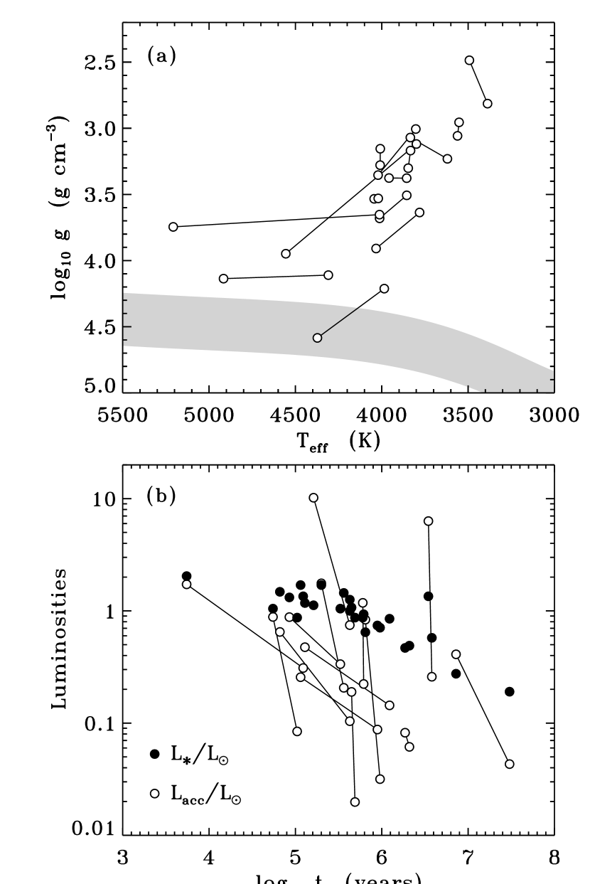
Figure 1.— Selection of derived stellar properties for the stars listed in Table 1. (a) Base-10 logarithm of surface gravity plotted against effective temperature (open circles), compared with the approximate position of the zero-age main sequence (gray band). (b) Stellar photon luminosity (filled circles) and accretion luminosity (open circles), both in units of the solar luminosity, shown as a function of age.

Figure 1 illustrates some stellar properties derived from the information given in Table 1. As in many of the plots in this paper, straight lines join together the independent determinations of quantities for each star that were computed from the HEG and HCGD pairs of rows in Table 1. The effective temperature $T_{\rm eff}$ and surface gravity $g=GM_{\ast}/R_{\ast}^{2}$ were computed assuming spherical symmetry. The accretion luminosity $L_{\rm acc}$ was estimated as $GM_{\ast}\dot{M}_{\rm acc}/R_{\ast}$, which ignores an order-unity correction factor for the free-fall from the inner edge of the disk (see Gullbring et al.  1998). Several points in these plots that show anomalous values deserve some extra mention.

1. The hottest star in the sample, with $T_{\rm eff}=5207$ K, corresponds to the HEG measurement for GM Aur. The HEG luminosity is about 2.3 times larger than the HCGD luminosity, which could account for both the larger effective temperature and its younger age. Other sources (e.g., Gullbring et al.  1998) report a luminosity that agrees better with the HCGD value, and thus it may be wise to ignore the HEG properties for this star.

2. The coolest and lowest-gravity star in Figure 1(a) is DF Tau. The HEG measurement has a slightly low gravity ($\log g=2.49$) when compared to other stars of similar age, but the HCGD measurements also indicate that its gravity is lower than average ($\log g=2.81$). The two sources agree about DF Tau being young (in age) and large (in radius), but the HEG value of the age ($\log t=3.74$) appeared to involve extrapolation beyond the range of ages used in the pre-main-sequence tracks of D’Antona & Mazzitelli (1994). Although this may have yielded an incorrect age, it does not affect the analysis of this paper, since the ages are not used as input parameters for any of the models.

3. There are two data points in Figure 1(b) with $L_{\rm acc}\gg L_{\ast}$. The HEG measurement of DO Tau (at $\log t=5.21$) exhibits the largest accretion rate of the sample in both sets of measurements, as well as the largest mass outflow rate and the largest value of $\delta$. Thus, DO Tau appears to be a genuinely active object. The other star with a large accretion luminosity is the HEG measurement of DS Tau (at $\log t=6.54$). Its accretion rate is typical, but it has an anomalously high ratio of $M_{\ast}/R_{\ast}$. HCGD also list DS Tau as the most massive star of this sample, but by less of a wide margin.

It should also be noted that the spread of measured ages for both the HEG and HCGD samples may be closely related to the episodic nature of the accretion. Intermittently variable accretion has been shown recently by Baraffe et al.  (2009) to produce a realistic spread of luminosities, such that a population of stars with identical ages $t\approx 1$ Myr may be interpreted (via standard evolutionary tracks) to have an age spread of as much as 10 Myr. In any case, the ages reported in Table 1 are used in this paper only to organize the data in graphical form, and not as inputs to the models.

The accretion rates given in Table 1 show a large degree of intrinsic scatter, even for stars of similar age and mass (see also Muzerolle et al.  2003; Calvet et al.  2004; Nguyen et al.  2009). In the earliest stages of star formation, this scatter may be the result of an inhomogeneous cluster environment (Pfalzner et al.  2008). For CTTS, however, this observational scatter is also likely to be the result of time variability in the three-dimensional pattern of magnetospheric accretion streams that connect the star and its surrounding disk. In any case, the observed values of $\dot{M}_{\rm acc}$ represent snapshots of the accretion that should ideally be paired with simultaneous measurements of the wind’s mass loss rate and X-ray activity. The observations used in this paper are not tightly constrained to be exactly contemporaneous, but in many cases the substantial uncertainty in these values lessens the importance of this issue.

The fraction of stellar surface area $\delta$ covered by accretion streams was computed for each star by Calvet & Gullbring (1998). They compared observed and modeled spectral energy distributions (i.e., Balmer and Paschen continua) to match both the total accretion energy flux and the emitting area on the stellar surface. There was no clear trend with age in these determinations of $\delta$, nor was there in the earlier measurements of Valenti et al.  (1993). It is important to note that both other observational diagnostics (Costa et al.  2000; Batalha et al.  2002; Donati et al.  2007) as well as some simulations (Romanova et al.  2004) have given rise to larger accretion-spot filling factors up to 10% or more. It is possible that these diagnostics may probe not just the magnetic flux tubes filled by the densest clumps, but also larger surrounding volumes that are energized by nearby accretion impacts (see also Brickhouse et al.  2009).

The surface magnetic field strengths $B_{\ast}$ shown in Table 1 were measured by Johns-Krull (2007) via the Zeeman broadening of several Ti I lines in the infrared. Only 10 of the 14 stars were observed, and for the other four we estimated their photospheric field strengths by assuming a mean level of partitioning between gas pressure and magnetic pressure (see below).

The mass loss rates $\dot{M}_{\rm wind}$ given in Table 1 were computed by HEG from the properties of high-velocity blueshifted emission components in forbidden lines such as [O I] $\lambda$6300 (see also Kwan & Tademaru 1995; Hartigan et al.  2004). These values have uncertainties of up to an order of magnitude. HEG reported only upper limits for BP Tau, DS Tau, and GM Aur, and these are not included in Table 1. It is uncertain whether these measured “jet” outflows originate on the stellar surface or in the accretion disk (see, e.g., Paatz & Camenzind 1996; Calvet 1997; Ferreira et al.  2006; Azevedo et al.  2007; Fendt 2009). If the empirical mass loss rates represent measurements of the outflow far from the stellar surface, then it is possible that they probe the sum of the mass fluxes from winds rooted both on the star and in the disk. In that case, these rates can be assumed to be tentative upper bounds for the stellar wind component.

The 28 sets of fundamental parameters from Table 1 were used to compute the photospheric mass densities $\rho_{\ast}$ at the surfaces of the T Tauri stars. The relevant criterion is that the Rosseland mean optical depth should have a value of approximately one (i.e., $\tau_{\rm R}\approx\kappa_{\rm R}\rho_{\ast}H_{\ast}=1$) at the stellar photosphere. The scale height $H_{\ast}$ is defined for simplicity as

$$H_{\ast}\,=\,\frac{c_{s}^{2}}{\gamma g}\,=\,\frac{k_{\rm B}T_{\rm eff}}{gm_{\rm H}}$$ (1)

where $c_{s}$ is the sound speed, $g$ is the surface gravity, $\gamma=5/3$ for an adiabatic gas, $k_{\rm B}$ is Boltzmann’s constant, and $m_{\rm H}$ is the mass of a hydrogen atom. The Rosseland mean opacity $\kappa_{\rm R}$ was interpolated as a function of temperature and density from the tables of Ferguson et al.  (2005). Figure 2 shows these derived photospheric densities along with other densities measured higher in the accretion streams that are defined below.

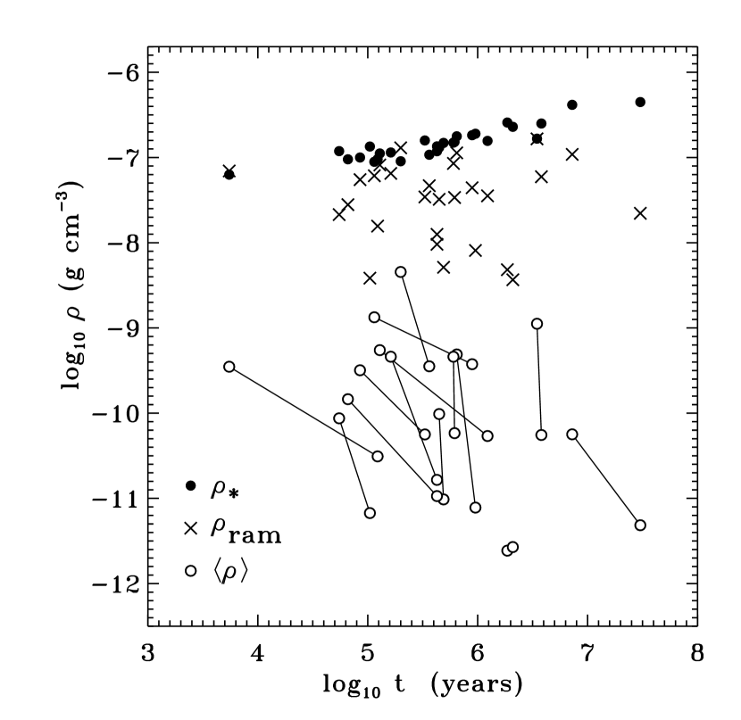
Figure 2.— Mass densities, plotted as a function of age, at the stellar photosphere (filled circles), at the accretion shock (crosses), and averaged over clumps and inter-clump regions in the accretion streams (open circles).

For each star with a measured magnetic field strength, the magnetic pressure $B_{\ast}^{2}/8\pi$ was compared to the photospheric gas pressure $P_{\ast}=\rho_{\ast}k_{\rm B}T_{\rm eff}/m_{\rm H}$. The equipartition field strength $B_{\rm eq}$ is defined as the field strength required to produce a magnetic pressure equal to the gas pressure. For the 10 stars (i.e., 20 rows of Table 1) for which this comparison could be made, the resulting values of the ratio $B_{\ast}/B_{\rm eq}$ ranged between 0.79 and 4.26. The mean value of the ratio was 2.084 and its standard deviation was 0.90. Thus, for the remaining four stars without magnetic field measurements, the magnetic field strength was estimated using this mean value $B_{\ast}=2.084B_{\rm eq}$.

3. Properties of Accretion Streams and Waves

During the CTTS phase, accretion of matter is believed to occur via supersonic ballistic infall along magnetic flux tubes that thread the inner disk (see Lynden-Bell & Pringle 1974; Uchida & Shibata 1984; Camenzind 1990; Königl 1991). The models developed in this paper make use of the idea that the accretion streams are likely to be highly unstable and time-variable, and thus much of the gas deposited onto the star is expected to be in the form of intermittent clumps (e.g., Gullbring et al.  1996; Safier 1998; Bouvier et al.  2003, 2004, 2007; Stempels 2003; Giardino et al.  2007). Although most of the observed CTTS photometric variability appears to be related to rotation of accretion streams and spots (with timescales of days), there is also persistent low-level hour-timescale variability that may reflect the internal clumpiness of the streams. Cranmer (2008) predicted that the number of accretion-related flux tubes on the stellar surface is likely to be of order $10^{2}$, such that if Poisson-like statistics dominated the distribution of clumps, the relative variability would be only of order 10%. This is within the realm of the observed hour-timescale variability (see, e.g., Rucinski et al.  2008; Nguyen et al.  2009).

As described by Scheurwater & Kuijpers (1988) and Cranmer (2008), the impact of each clump is expected to generate MHD waves and turbulence on the stellar surface. When these fluctuations propagate across the surface, they spread out the kinetic energy of accretion and inject some of it into the star’s global magnetic field. This analysis neglects possible additional motions that could be driven by instabilities in the accretion shock itself (e.g., Chevalier & Imamura 1982; Mignone 2005). For strong enough magnetic fields on CTTS surfaces, these instabilities appear to be suppressed (Koldoba et al.  2008). However, in some simulations there are long-term transitions between periods of stability and instability (Romanova et al.  2008).

The dynamical properties of accretion streams are modeled here assuming ballistic infall—from the inner edge of the accretion disk—along field lines described by an axially symmetric dipole (e.g., Calvet & Hartmann 1992; Muzerolle et al.  2001). Although we know that the actual magnetic fields of T Tauri stars can have non-dipolar components (Donati et al.  2007; Gregory et al.  2008), the dipole assumption allows representative geometrical properties of the streams to be calculated easily. In the absence of explicit specification below, the parameters and methods used to model the accretion streams are the same as those of Cranmer (2008).

The field lines that thread the disk intercept the equatorial plane between inner and outer radii $r_{\rm in}$ and $r_{\rm out}$. The location of the inner radius (also called the truncation radius) is specified here using Königl’s (1991) assumption of pressure balance between the accretion stream and the stellar magnetic field, with

$$r_{\rm in}\,=\,0.5\left(\frac{B_{\ast}^{4}R_{\ast}^{12}}{2GM_{\ast}\dot{M}_{\rm acc}^{2}}\right)^{1/7}\,\,.$$ (2)

The outer radius can be computed if we know the fraction of the stellar surface $\delta$ that is covered by the accretion streams. For a dipole field, these quantities satisfy

$$\sqrt{1-\frac{R_{\ast}}{r_{\rm out}}}\,=\,\delta+\sqrt{1-\frac{R_{\ast}}{r_{\rm in}}}\,\,.$$ (3)

A field line that intersects the disk at a radius $r>r_{\rm in}$ encounters the stellar surface at a colatitude $\theta$, where $\sin^{2}\theta=R_{\ast}/r$. Thus, the radii $r_{\rm in}$ and $r_{\rm out}$ correspond to surface colatitudes $\theta_{\rm in}$ and $\theta_{\rm out}$, respectively.

For the stellar properties listed in Table 1, the ratio $r_{\rm in}/R_{\ast}$ ranges between 1.3 and 8. These values correspond roughly to the highest and lowest accretion rates, respectively. The ratio $r_{\rm out}/r_{\rm in}$ ranges between 1.006 and 1.81 (with a median value of 1.066). The mean colatitudes of the accretion streams range from about 20°, for the oldest stars with the lowest accretion rates, to 60°, for the youngest stars with highest accretion rates. The fractional surface area covered by the “polar caps” $\delta_{\rm pol}$ (i.e., the regions between colatitudes 0 and $\theta_{\rm out}$ on each pole) does not vary significantly with age, and its mean value for all of the stars is about 0.15. The fractional surface area covered by the equatorial band of closed magnetic fields (i.e., $\delta_{\rm equ}=1-\delta-\delta_{\rm pol}$) has an average value of about 0.83. Although these numbers depend on the assumption of dipole symmetry, they are more empirically grounded than the models of Cranmer (2008). In that paper, both the ratio $r_{\rm out}/r_{\rm in}$ and the surface field strength $B_{\ast}$ were specified as arbitrary constants, but here they are based on specific measurements for each star.

The accreting gas is accelerated from rest at the inner edge of the disk to a ballistic free-fall speed at the stellar surface,

$$v_{\rm ff}\,=\,\left[\frac{2GM_{\ast}}{R_{\ast}}\left(1-\frac{R_{\ast}}{r_{\rm in}}\right)\right]^{1/2}\,\,.$$ (4)

This expression slightly underestimates the mean free-fall velocity, since the streams actually come from all radii between $r_{\rm in}$ and $r_{\rm out}$. The free-fall speeds at the stellar surface range between 100 and 600 km s^-1, and they increase with increasing age roughly as $t^{0.22}$ because of a similar behavior in the stellar escape speed.

In the models of Cranmer (2008) it was assumed that the free-fall speed $v_{\rm ff}$ is identical to the speed of infalling clumps $v_{c}$ that occupy the accretion streams. Here, however, the wider range of stellar properties and accretion rates (in Table 1) necessitates a closer look at that assumption. Scheurwater & Kuijpers (1988) found that the optimal situation was for the clump’s ram pressure to be larger than the gas pressure in the stream, but smaller than the magnetic pressure. When these conditions are not met, the clumps may be decelerated (with $v_{c}<v_{\rm ff}$). Considering only the “stopping power” of a large ambient gas pressure, equation (64) of Scheurwater & Kuijpers (1988) gave an upper-limit clump speed of

$$v_{c}\,\leq\,\left(\frac{2}{3}\frac{r_{c}}{R_{\ast}}\frac{\rho_{c}}{\rho_{0}}\right)^{1/2}v_{\rm ff}$$ (5)

where $r_{c}\approx R_{\ast}(\theta_{\rm in}-\theta_{\rm out})/2$ is the radius of a representative spherical clump at the surface, $\rho_{c}$ is the density interior to each clump, and $\rho_{0}$ is the ambient density between clumps in the accretion streams. The Cranmer (2008) models did not depend explicitly on the ratio $\rho_{c}/\rho_{0}$, but here it needs to be computed.

A first estimate of the density contrast of supersonically accelerated clumps may involve the fact that such features could easily form shocks in the accretion streams. In that case, the maximum density contrast would be of order $(\gamma+1)/(\gamma-1)\approx 4$, with $\gamma=5/3$ for an adiabatic gas. However, Elmegreen (1990) showed that MHD waves can form in this kind of infall-dominated region and lead to the occurrence of colliding nonlinear wave packets. These can efficiently clear out the gas from the inter-clump regions and thus enhance the density contrast up to factors of order 100. Note that if we assumed that $\rho_{c}/\rho_{0}\rightarrow\infty$, the upper limit in equation (5) would never be applied. On the other hand, assuming too low a value for the density contrast ratio would lead to an unrealistic over-application of this limit. Thus, a conservative approach would be to use a value for this ratio that may err on the side of being too large. In the absence of other information, the trial value of 100 was chosen. This ends up reducing $v_{c}$ below $v_{\rm ff}$ in the majority of cases (20 out of 28) by about a factor of two, and allowing $v_{c}=v_{\rm ff}$ in the other 8 cases.

The other possible deceleration effect involves a comparison between the clump’s ram pressure and the magnetic pressure of the accretion stream. The theoretical development of Scheurwater & Kuijpers (1988) and Cranmer (2008) assumed that the passage of a clump does not disrupt the mean magnetic field in the stream. However, if a clump’s ram pressure begins to exceed the local magnetic pressure, MHD instabilities may occur that further decelerate the clump to a point where it can no longer disrupt the field. Thus, for each star, we made sure that $v_{c}$ never exceeds half of the intra-clump Alfvén speed $B_{0}/(4\pi\rho_{c})^{1/2}$ (see equation [1] of Scheurwater & Kuijpers 1988). This further reduction was applied in 10 out of the 28 cases, and the final saturated values of $v_{c}$ were found to range between about 30 and 530 km s^-1.

The accretion streams are assumed to be stopped at the location where the ram pressure,

$$P_{\rm ram}\,=\,\frac{\rho v_{c}^{2}}{2}\,=\,\frac{v_{c}\dot{M}_{\rm acc}}{8\pi\delta R_{\ast}^{2}}\,\,,$$ (6)

is balanced by the gas pressure of the undisturbed stellar atmosphere (e.g., Hartmann et al.  1997; Calvet & Gullbring 1998). This paper uses a new algorithm to estimate the density $\rho_{\rm ram}$ at which this balance occurs. The approximation given by Cranmer (2008)—who used the notation $\rho_{\rm sh}$ for this quantity—assumed that the ram pressure balance occurs well above the photosphere, such that the temperature has reached its minimum value of approximately $\sim 0.84T_{\rm eff}$ (for radiative equilibrium in a gray atmosphere). However, larger accretion rates imply that the accretion shock may penetrate deeper into higher-temperature regions. The new prescription uses a gray atmosphere relation for temperature versus optical depth (Mihalas 1978), with

$$T^{4}\,=\,\frac{3}{4}T_{\rm eff}^{4}\left(\tau+\frac{2}{3}\right)$$ (7)

and the height dependence of the optical depth $\tau$ is approximated via hydrostatic equilibrium and a constant opacity; i.e., $\tau(z)\approx\kappa\rho(z)H_{\ast}$. In this case, the ram pressure balance condition is given by

$$P_{\rm ram}\,=\,0.84P_{\ast}e^{-z_{\rm ram}/H_{\ast}}\left(1+e^{-z_{\rm ram}/H_{\ast}}\right)^{1/4}$$ (8)

where $z_{\rm ram}$ is the height of ram pressure balance that must be solved for numerically. Once $z_{\rm ram}$ has been determined, the density at this height is given straightforwardly by $\rho_{\rm ram}=\rho_{\ast}e^{-z_{\rm ram}/H_{\ast}}$. The approximate version given in equation (10) of Cranmer (2008) is equivalent to ignoring the final exponential term in equation (8) above. Figure 2 shows $\rho_{\rm ram}$ for the stars modeled in this paper. Note that the shock penetrates below the photosphere ($\rho_{\rm ram}>\rho_{\ast}$) for only two of the 28 data points; these are the HEG values of DF Tau and DK Tau.

The energy in Alfvén waves released on the stellar surface from a single clump impact was given by Scheurwater & Kuijpers (1988) as

$$E_{\rm A}\,=\,0.06615\,\,\frac{\rho_{c}}{\rho_{0}}\left(\frac{v_{c}}{V_{\rm A}}\right)^{3}m_{c}v_{c}^{2}$$ (9)

where $m_{c}$ is the mass in the clump and the Alfvén speed $V_{\rm A}$ is defined as that of the ambient medium, with $V_{\rm A}=B_{0}/(4\pi\rho_{0})^{1/2}$. Because these equations are applied near the stellar surface, the magnetic field strength in the accretion stream $B_{0}$ is assumed to be equal to $B_{\ast}$. Cranmer (2008) worked out the conversion from a single clump’s wave energy yield to the time-steady amplitude of Alfvén waves (from the continuous accretion of many clumps) at the north and south poles of a star with a dipole field geometry. Using equations (19)–(22) of Cranmer (2008), the transverse velocity amplitude of waves in the polar photosphere can be written as

$$v_{\perp\ast}\,=\,0.5145\left(\frac{\langle\rho\rangle\rho_{\rm ram}\delta}{\rho_{c}\rho_{\ast}\Delta\theta}\right)^{1/2}\frac{v_{c}^{3}}{B_{\ast}^{2}/(4\pi\rho_{c})}$$ (10)

where $\Delta\theta=(\theta_{\rm in}-\theta_{\rm out})(\theta_{\rm in}+\theta_{\rm out})$ and the time-averaged mean density in the accretion streams is

$$\langle\rho\rangle\,=\,\frac{\dot{M}_{\rm acc}}{4\pi\delta R_{\ast}^{2}v_{c}}\,\,.$$ (11)

This quantity is intermediate between $\rho_{0}$ and $\rho_{c}$, and it is plotted in Figure 2 for the 28 stellar data points. The total flux of Alfvén waves at the pole is given by $F_{\rm A}=\rho_{\ast}v_{\perp\ast}^{2}V_{{\rm A}\ast}$, where $V_{{\rm A}\ast}=B_{\ast}/(4\pi\rho_{\ast})^{1/2}$. The fluxes of waves that reach other regions on the stellar surface (away from the poles) are discussed in Sections 4 and 6.

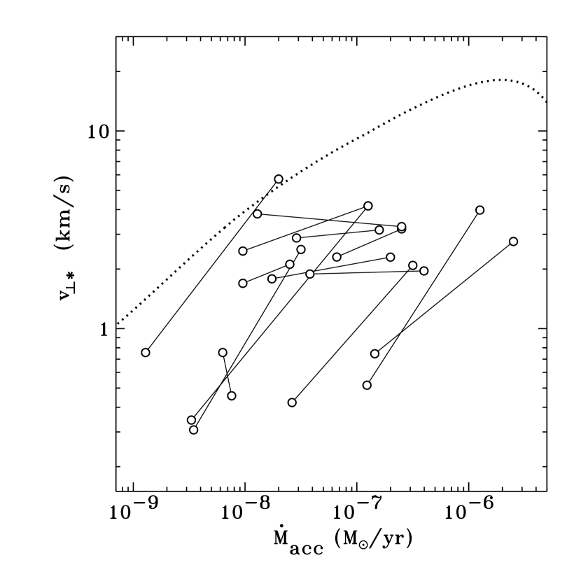
Figure 3.— Photospheric velocity amplitudes of Alfvén waves induced by magnetospheric accretion, plotted as a function of the accretion rate. Wave velocities were computed at the north and south poles for the stars listed in Table 1 (open circles) and for the model evolutionary sequence of a 1 $M_{\odot}$ star from Cranmer (2008) (dotted line).

Figure 3 shows the Alfvén wave velocity amplitude for each star as a function of the accretion rate. Also shown is the continuous relationship for the idealized evolutionary sequence of a 1 $M_{\odot}$ star from Cranmer (2008). The wave amplitudes derived for the current stellar sample are generally lower than those from Cranmer (2008). Part of this is due to the new models taking into account the two ram-pressure-deceleration effects that were discussed above. Also, it should be noted that the average stellar mass for the stars in Table 1 is less than 1 $M_{\odot}$, so even the unmodified free-fall speeds $v_{\rm ff}$ were generally lower than those of Cranmer (2008).

4. Stellar Winds from Polar Regions

For several decades, MHD waves have been studied as likely sources of energy and momentum for accelerating winds from cool stars (see, e.g., Hollweg 1978; Hartmann & MacGregor 1980; DeCampli 1981; Wang & Sheeley 1991; Airapetian et al.  2000; Falceta-Gonçalves et al.  2006; Suzuki 2007). The models of polar T Tauri winds developed by Cranmer (2008) involved two sources for the MHD waves at the photosphere: (1) convection-generated waves that propagate up from the interior, and (2) accretion-generated waves of the form discussed in Section 3. The Alfvén waves were assumed to propagate up the open field lines, dissipate via an MHD turbulent cascade, and heat the plasma over an extended range of distance. The resulting winds that had low (solar-type) mass loss rates were driven by a combination of coronal gas pressure and wave pressure. The high mass-loss winds of the youngest stars, however, were radiatively cooled to chromospheric ($T\sim 10^{4}$ K) temperatures and thus were dominated by wave pressure. This paper makes the assumption that the T Tauri stars of Table 1 correspond to the latter physical regime of cool, wave-driven winds.

It was not possible to simply apply the cool-wind modeling technique of Cranmer (2008) in this paper. That methodology depended on knowing the exact values for several parameters that cannot be reliably estimated for the present database of T Tauri stars. For example, many of the details of the numerical wind models depended on the photospheric filling factor of magnetic flux tubes. The models of Cranmer (2008) used a low filling factor that is appropriate for the present-day Sun, but possibly not for young CTTS. Furthermore, the analytic young-star model described in Sections 5.2 and 5.3 of Cranmer (2008) relied on an empirical extrapolation of the Alfvén wave amplitude at the critical point from the numerical models of older stars in the evolutionary sequence. The general cool wave-driven wind theory of Holzer et al.  (1983) thus needed to be reanalyzed and adapted for the observational stellar sample discussed above.

Before discussing the wind model, however, there is one modification of the lower boundary condition on $v_{\perp\ast}$ that should be specified. Equation (10) gives the photospheric Alfvén wave amplitude at the north or south pole of the magnetic stellar dipole. Using this value would give the properties of the stellar wind only over the poles. But in order to compute the total mass loss rate $\dot{M}_{\rm wind}$ that comes from the open fields spanning the two polar cap regions, we decided to average over these polar caps. The wave flux from equation (10) is thus multiplied by the following correction factor

$$C_{\rm pol}\,=\,\frac{1}{\delta_{\rm pol}}\int_{0}^{\theta_{\rm out}}d\theta\,\sin\theta\,\,\frac{F_{\rm A}(\theta)}{F_{\rm A}(0)}\,\,.$$ (12)

The expressions given in Section 3.4 of Cranmer (2008) are required to compute the latitude dependent wave flux $F_{\rm A}(\theta)$. The polar value of $v_{\perp\ast}$ is multiplied by $C_{\rm pol}^{1/2}$ to produce the mean value for the entire polar-cap region.

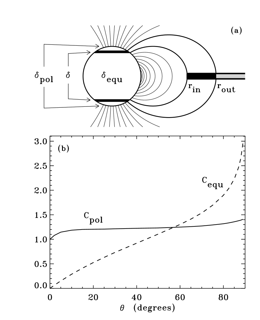
Figure 4.— (a) Modeled magnetic field geometry, showing inner and outer equatorial radii $r_{\rm in}$ and $r_{\rm out}$ between which accretion takes place, as well as fractional areas on the stellar surface subtended by accretion streams ($\delta$), open-field polar caps ($\delta_{\rm pol}$), and equatorial closed-field loops ($\delta_{\rm equ}$). (b) Correction factors for photospheric Alfvén wave fluxes plotted versus the mean colatitude $\theta$ of accretion streams on the surface. $C_{\rm pol}$ and $C_{\rm equ}$ specify ratios of surface-averaged wave flux (with the averages taken over the polar and equatorial regions, respectively) to the wave flux at the poles.

Figure 4 illustrates the relevant geometry and how $C_{\rm pol}$ varies as a function of the mean polar-cap latitude $(\theta_{\rm in}+\theta_{\rm out})/2$. Note that the application of this correction factor gives rise to slightly larger wave amplitudes than those shown in Figure 3. The averaging over the entire polar cap includes points on the stellar surface that are closer to the accretion ring which have larger local wave amplitudes. However, the magnitude of the $C_{\rm pol}$ correction factor is never far from unity, and thus it gives rise to only a relatively small change in $v_{\perp\ast}$. It is included here for consistency with the use of a corresponding equatorial correction factor $C_{\rm equ}$ that is more important when computing the properties of the closed low-latitude loops (see Section 6).

The calculation of the stellar wind’s mass loss rate largely follows the development of Holzer et al.  (1983). Two key assumptions are: (1) that the Alfvén wave amplitudes are larger than the sound speeds in the wind, and (2) that there is negligible wave damping between the stellar surface and the wave-modified “critical point” of the flow. A third assumption from Holzer et al.  (1983)—which was initially not applied but later found to be valid—is that the stellar wind is sub-Alfvénic at the critical point (i.e., that the wind speed is much smaller than $V_{\rm A}$ at the critical point). A first round of numerical models was constructed without the third assumption. These models integrated the equation of motion up and down from the critical point, and used an iteration technique to determine the true critical point radius $r_{\rm crit}$. However, the resulting values of $r_{\rm crit}$ always remained close to the numbers given by equation (35) of Holzer et al.  (1983), in which all three of the above assumptions were applied. This expression,

$$\frac{r_{\rm crit}}{R_{\ast}}\,\approx\,1+\frac{3}{2}\left(\frac{d\ln A}{d\ln r}\right)^{-1}\,\,,$$ (13)

was thus used in the models described below, where $A(r)$ describes how the cross-sectional area of the open magnetic flux tubes varies with distance. For a dipole geometry over the poles, $A\propto r^{3}$ and $r_{\rm crit}\approx 1.5\,R_{\ast}$. The current models assume that the filling factor of magnetic flux tubes at the photosphere is unity (see, e.g., Saar 2001).

Once the critical point radius is known, it becomes possible to use the same kinds of arguments as used in Section 5.3 of Cranmer (2008) to estimate the wind velocity and density at the critical point, and thus to compute the mass loss rate. There are three unknown quantities and three equations to constrain them. The three unknowns are the critical point values of the wind speed $u$, density $\rho$, and wave amplitude $v_{\perp}$. The first equation is the constraint that the right-hand side of the time-steady momentum equation must sum to zero at the critical point of the flow (see, e.g., Parker 1958, 1963). For the conditions described above, this gives

$$\frac{GM_{\ast}}{r_{\rm crit}^{2}}\,=\,\frac{3u_{\rm crit}^{2}}{r_{\rm crit}}$$ (14)

and it is solved straightforwardly for $u_{\rm crit}$. The second and third equations are, respectively, the definition of the critical point velocity (in the “cool” limit of zero gas pressure)

$$u_{\rm crit}^{2}\,=\,\frac{v_{\perp}^{2}}{4}\left(\frac{1+3M_{\rm A}}{1+M_{\rm A}}\right)$$ (15)

and the conservation of wave action

$$\rho v_{\perp}^{2}V_{\rm A}(1+M_{\rm A})^{2}A\,=\,\mbox{constant}$$ (16)

where $M_{\rm A}=u/V_{\rm A}$ is the Alfvén Mach number (see, e.g., Jacques 1977). The constant in equation (16) is known for each star because the conditions at the photosphere are known (and it is also valid to assume $M_{\rm A}\rightarrow 0$ there as well). The wave amplitude $v_{\perp}$ in equations (15) and (16) is evaluated at the critical point, where the conservation of wave action gives rise to much larger values than those at the photosphere (i.e., $v_{\perp}\gg v_{\perp\ast}$).

The fact that $V_{\rm A}$ itself depends on the density makes it difficult to find an explicit analytic solution for $\rho_{\rm crit}$. Instead, the model code used here starts with a reasonable initial guess and solves equations (13)–(16) iteratively until consistency is reached. The resulting iterated values for $v_{\perp}$ at the critical point range between 85 and 425 km s^-1. In all cases, these Alfvén wave amplitudes are larger than the sound speeds in a cool chromospheric wind. The resulting values for $\rho_{\rm crit}$ span more than five orders of magnitude between $10^{-18}$ and $4\times 10^{-13}$ g cm^-3.

The stellar wind’s mass loss rate was determined by applying the equation of mass conservation and taking into account that the open fields over the polar caps have widened by the time that the wind reaches $r_{\rm crit}$. For a dipole geometry, a rough estimate of this widening factor is $\delta_{\rm crit}\approx\delta_{\rm pol}(r_{\rm crit}/R_{\ast})^{3}$. However, for two out of the 28 cases from Table 1, this approximation gives a number greater than 1. For these two cases the value of $\delta_{\rm crit}$ was simply assumed to be 1. Thus, the mass loss rate is estimated as $\dot{M}_{\rm wind}=4\pi r_{\rm crit}^{2}\delta_{\rm crit}u_{\rm crit}\rho_{\rm crit}$.

Table 2Modeled Wind, Shock, & Coronal Loop Properties

	log $\dot{M}_{\rm wind}$	log $T_{\rm sh}$	log $n_{\rm post}$	$\langle L\rangle$	log $T_{\rm max}$	log $n_{\rm TR}$	log $n_{\rm top}$
Object	($M_{\odot}/\mbox{yr}$)	(K)	(cm-3)	(Mm)	(K)	(cm-3)	(cm-3)	$\alpha_{\rm R}$
AA Tau	–8.61	5.163	15.04	28.9	6.99	13.60	10.61	1.74
	–13.66	5.892	13.27	18.6	6.75	12.86	10.11	1.98
BP Tau	–9.10	4.986	15.01	27.0	6.91	13.36	10.45	1.77
	–9.50	5.662	14.14	25.6	6.90	13.32	10.42	1.80
CY Tau	–12.24	6.170	12.76	12.3	6.57	12.32	9.75	1.95
	–12.79	5.982	12.80	22.0	6.58	12.35	9.78	1.97
DE Tau	–8.90	5.125	14.29	94.4	6.82	13.09	10.27	1.77
	–12.19	5.583	13.20	74.3	6.70	12.72	10.02	1.96
DF Tau	–7.50	5.194	14.90	235.2	7.16	14.11	10.95	1.68
	–11.68	5.521	13.86	105.4	7.00	13.63	10.63	1.95
DK Tau	–9.55	4.305	15.84	52.0	7.00	13.63	10.63	1.82
	–10.04	5.053	14.90	41.5	6.97	13.54	10.57	1.85
DN Tau	–9.55	5.416	14.36	34.5	6.90	13.32	10.42	1.81
	–13.46	5.585	13.36	35.6	6.73	12.81	10.08	1.98
DO Tau	–8.70	4.916	15.00	58.2	6.95	13.49	10.53	1.74
	–11.62	5.745	13.59	40.5	6.86	13.21	10.34	1.93
DS Tau	–9.79	4.810	15.37	7.9	6.88	13.25	10.38	1.80
	–9.78	5.955	14.12	7.4	6.90	13.32	10.42	1.81
GG Tau	–8.96	4.997	14.51	84.8	6.85	13.16	10.32	1.77
	–10.13	5.835	13.40	41.9	6.77	12.92	10.16	1.84
GI Tau	–8.28	5.100	15.09	62.1	7.05	13.77	10.72	1.72
	–10.52	5.767	14.10	10.0	6.87	13.24	10.37	1.86
GM Aur	–10.56	4.594	15.41	18.2	6.87	13.23	10.36	1.85
	–10.64	4.992	14.92	19.6	6.84	13.16	10.31	1.89
HN Tau	–9.01	6.176	14.13	6.4	6.96	13.51	10.55	1.76
	–13.41	6.570	13.06	2.2	6.70	12.73	10.03	1.98
UY Aur	–8.53	5.008	14.85	73.8	6.95	13.48	10.53	1.73
	–9.37	5.637	14.12	46.6	6.95	13.46	10.52	1.81

Table 2 gives the resulting mass loss rates for the 28 stars in the observational database, and Figure 5(a) plots the ratio $\dot{M}_{\rm wind}/\dot{M}_{\rm acc}$ as a function of age. The observationally determined mass loss rates from blueshifted [O I] $\lambda$6300 lines (HEG) are also shown, as are the model results for the idealized evolutionary sequence of a 1 $M_{\odot}$ star (Cranmer 2008). Of the 22 cases (11 stars) where it is possible to compare directly with measured mass loss rates, 7 of the computed values are within an order of magnitude of the observed rates. The majority of the cases (17 out of 22) have lower modeled rates than the observations, and only 5 have higher values. For all 22 cases, the median value of the ratio of modeled to measured $\dot{M}_{\rm wind}$ is 0.08. As discussed further below, this implies that the outflows probed by the [O I] diagnostic may be dominated by the disk wind component, which is not modeled here.

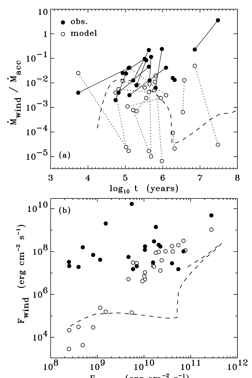
Figure 5.— (a) Stellar wind mass loss rates, normalized by the accretion rates for each star, plotted versus age. (b) Energy flux in the stellar wind plotted against the energy flux in Alfvén waves on the stellar surface. The model calculations of this paper (open circles) are compared with the HEG observations (filled circles) and the modeled evolutionary sequence of Cranmer (2008) (dashed line).

Figure 5(b) compares the input flux of Alfvén waves at the photosphere with the computed energy flux of the stellar wind. The Alfvén wave flux $F_{\rm A}=F_{\rm wave}$ was defined in Section 3, and the wind’s energy flux is estimated to be

$$F_{\rm wind}\,\approx\,\frac{L_{\rm wind}}{4\pi R_{\ast}^{2}}\,=\,\frac{GM_{\ast}\dot{M}_{\rm wind}}{4\pi R_{\ast}^{3}}\,\,.$$ (17)

The above quantity includes only the energy required to lift the wind out of the star’s gravity well, and not to accelerate it up to its asymptotic terminal speed. Thus it is not the total energy flux of the wind. Note also that equation (17) does not use any of the polar-cap area factors defined above (e.g., $\delta_{\rm pol}$ or $\delta_{\rm crit}$) because the wind luminosity $L_{\rm wind}$ is presumably defined at an infinite distance where the flux tubes have opened up to fill most of the circumstellar volume. However, as long as a consistent definition is used for the various quantities plotted in Figure 5(b), they can be compared with one another fairly.

The fact that the modeled values of $F_{\rm wind}$ show a clear correlation with $F_{\rm wave}$ in Figure 5(b) is not surprising, since these winds are assumed to be wave-driven. The dashed curve, from the evolutionary sequence of Cranmer (2008), also shows a similar correlation. The wind fluxes from Cranmer (2008) are generally lower than those computed in this paper because the former models used a relatively small filling factor for the magnetic flux tubes at the photosphere. Smaller filling factors lead to more dilution of the wave energy between the surface and the critical point of the wind, and thus to less energy deposition overall.

In Figure 5(b), the model data points appear to be subdivided into two groups, with a diving line around $F_{\rm wind}\approx 10^{6}$ erg cm^-2 s^-1. The group with the larger wind fluxes has a lower limit that is close to the lower limit of the observed values. Out of the 28 cases, 20 of the modeled wind fluxes fall into this upper group, and only 8 are in the group that falls well short of the observationally constrained wind fluxes. At first glance, this may appear inconsistent with the fact that approximately 77% of the data points shown in Figure 5(a) (i.e., 17 out of 22) have modeled ratios $\dot{M}_{\rm wind}/\dot{M}_{\rm acc}$ that are lower than the observed ratios. However, the 77% fraction was computed by comparing each model data point individually with its corresponding observation. The corresponding 29% fraction above (8 models out of 28 that under-predict the observations) was found by examining the overall distribution of points in Figure 5(b) and not matching up the results for each star. Also, the wind flux does not depend strongly on the accretion rate, but $\dot{M}_{\rm acc}$ appears explicitly in the denominator of the ratio shown in Figure 5(a). The measured accretion rates show a large intrinsic range of variability that influences the overall statistical agreement or disagreement between the models and observations.

As also found by Cranmer (2008), many of the predicted mass loss rates fall below those determined from the [O I] observations of HEG. However, the level of limited agreement with the data is interesting, because the measured mass loss rates are widely believed to sample the much larger-scale disk wind or X-wind. It is thus possible that, for some stars, stellar winds may contribute to observational signatures that are typically associated only with bipolar jets rooted in the accretion disk.

It is evident from Figure 5(a) that the pair of models for a given star (i.e., the models for the HEG and HCGD values of the observed parameters) can have drastically different predictions for the stellar wind properties. For many of the stars, the observational uncertainties drive the uncertainties in the models. Thus, it is worthwhile to ask which of the measured parameters are most responsible for these large discrepancies. Since the modeled $F_{\rm wind}$ is well correlated with $F_{\rm wave}$, one can use equations (6)–(11) in Section 3 to work out an approximate scaling relation for how $F_{\rm wave}$ depends on the empirical input parameters. If one also assumes $F_{\rm wind}\propto F_{\rm wave}^{1.87}$ (see Figure 5(b)), then equation (17) can be used to estimate

$$\dot{M}_{\rm wind}\propto\,\left(\frac{\dot{M}_{\rm acc}}{B_{\ast}\delta}\right)^{5.62}\frac{v_{c}^{9.37}}{M_{\ast}R_{\ast}^{8.24}}\,\,,$$ (18)

where it was found that the angular factor $\Delta\theta$ is roughly proportional in magnitude to $\delta$, and small variations in the stellar $\rho_{\ast}$ and $T_{\rm eff}$ are neglected. The two most sensitive factors are the infalling clump speed $v_{c}$ (which is related to the freefall speed $v_{\rm ff}$) and the stellar radius $R_{\ast}$. However, the accretion rate $\dot{M}_{\rm acc}$, the accretion spot filling factor $\delta$, and the surface magnetic field strength $B_{\ast}$ are also non-negligible contributors. It is difficult to isolate just one or two of the observations in, e.g., Table 1, that if improved would drastically improve the model predictions.

It is also possible that the theoretical mass fluxes have been underestimated systematically. For example, the efficiency of conversion from the kinetic energy of infalling clumps to MHD wave energy on the stellar surface (equation 9) was computed by Scheurwater & Kuijpers (1988) in the “far-field” limit. This approximation neglects energy near the base of the accretion stream that is transient in nature, or is associated with possible shocks, or is the result of center-to-edge inhomogeneities in the streams (see, e.g., Romanova et al.  2004). The actual efficiency thus may be larger than was assumed in equation (9). Also, if the stellar magnetic field has strong high-order multipole components (i.e., departures from a dipole), the surface may be peppered with a more evenly spread distribution of accretion spots than is assumed here. This would mean that the launching regions of the stellar wind may, on average, be closer to the nearest accretion spots, and thus the flux of MHD waves in these regions may be larger.

X-ray emission from the winds of T Tauri stars is generally considered to be negligible when compared with that of the nearby accretion shocks and closed-field coronal loops (see Figure 13 of Cranmer 2008). This is similar to the case of dark “coronal holes” on the surface of the Sun (e.g., Noci 1973; Zirker 1977; Cranmer 2009). In open-field regions containing an accelerating stellar wind, the density and pressure cannot build up to the higher levels found in more confined and static regions. The energy budget of the wind is thus dominated by the kinetic energy lost in the outflow itself, and comparatively little is left over for radiation at UV and X-ray wavelengths. This paper thus does not compute the X-ray fluxes from these polar open-field regions.

5. Accretion Shocks

The impact of magnetospheric accretion streams onto the stellar surface generates standing shocks. As the infall speeds are decelerated at the shock, both the temperature and density increase. There is also a postshock cooling zone, over which the density continues to increase but the temperature decreases back down to the undisturbed atmospheric value. These regions have been suggested as potential sources of soft X-rays for T Tauri stars (e.g., Lamzin 1999; Kastner et al.  2002; Grosso et al.  2007; Robrade & Schmitt 2007). Although the surface areas of these spots are believed to be small ($\delta\sim 0.01$), the ballistic impact speeds are high enough to generate temperatures of order 10⁵–10⁶ K.

The model of accretion shocks described here is a simplified version of similar one-dimensional models in the literature (Gullbring 1994; Calvet & Gullbring 1998; Günther et al.  2007; Sacco et al.  2008). Near the stellar surface, the magnetic field is assumed to be oriented radially, and we ignore any structure or dynamics transverse to the field. The preshock velocity and density in the accretion streams are given by $v_{1}=v_{c}$ and $\rho_{1}=\langle\rho\rangle$. The immediate postshock conditions $v_{2}$ and $\rho_{2}$ are computed from the standard Rankine-Hugoniot conditions (Landau & Lifshitz 1959) using an adiabatic ratio of specific heats $\gamma=5/3$. The determination of the shock height, with respect to the undisturbed stellar atmosphere, is described in Section 3.

Because the speed of infalling clumps $v_{c}$ is not necessarily highly supersonic, it is necessary to use the complete version of the shock-jump condition for the temperature,

$$c_{2}^{2}\,=\,\frac{5k_{\rm B}T_{\rm sh}}{3\langle m\rangle}\,=\,\frac{(5v_{1}^{2}-c_{1}^{2})(v_{1}^{2}+3c_{1}^{2})}{16v_{1}^{2}}$$ (19)

where $c_{1}$ is the sound speed in the accretion stream, $c_{2}$ is the postshock sound speed, and $\langle m\rangle\approx 0.6m_{\rm H}$ is the mean particle mass used here in order to more accurately determine $T_{\rm sh}$. We estimate $c_{1}=13.8$ km s^-1, which is consistent with a temperature in the accretion streams of $\sim$8000 K (see, e.g., Martin 1996; Muzerolle et al.  2001). The commonly used approximate version of equation (19) results when $c_{1}\rightarrow 0$.

Table 2 shows the postshock temperature $T_{\rm sh}$ and postshock number density $n_{\rm post}=\rho_{2}/m_{\rm H}$ for the 28 empirical stellar cases studied here. For these stars, the postshock temperatures range between about 0.02 and 4 MK. There is a trend with age that can be described roughly by

$$T_{\rm sh}\,\approx\,5.2\times 10^{5}\left(\frac{t}{1\,\,\mbox{Myr}}\right)^{0.42}\,\,\mbox{K}\,\,,$$ (20)

although there is substantial spread around this power-law variation especially at the youngest ages. It is important to note that the median value of $T_{\rm sh}$ is only 0.33 MK, and that there are only 3 out of 28 cases with $T_{\rm sh}\geq 1$ MK. This is lower than the typical values of 2–3 MK that have been inferred from soft X-ray observations associated with accretion shocks (e.g., Robrade & Schmitt 2007). It is possible that the reductions in the clump infall speed below the ballistic free-fall speed ($v_{c}<v_{\rm ff}$) described in Section 3 were overestimated. However, had these deceleration factors been neglected, the resulting models would have produced an unrealistically strong level of X-ray emission that disagrees with the observations (see Section 7).

The physical depth and structure of the postshock cooling zone were computed using the analytic model of Feldmeier et al.  (1997). This model assumes that the radiative cooling rate ($Q_{\rm rad}=n_{e}n_{\rm H}\Lambda(T)$) exhibits a power-law temperature dependence of $\Lambda\propto T^{-1/2}$. The cooling zone has a vertical thickness given by equation (9) of Feldmeier et al.  (1997), which can be expressed as

$$\Delta z\,=\,0.407\,\left(\frac{v_{2}}{50\,\,\mbox{km}\,\,\mbox{s}^{-1}}\right)^{4}\left(\frac{\rho_{2}}{10^{-10}\,\,\mbox{g}\,\,\mbox{cm}^{-3}}\right)^{-1}\,\,\mbox{km}\,\,.$$ (21)

For the T Tauri stars studied here, the thickness of the cooling zone ranges from about 10 cm (for the youngest stars) to 100 km (for the oldest stars). The spatial dependence of density, temperature, and velocity in the cooling zone is specified by equations (8)–(11) of Feldmeier et al.  (1997), and the shapes of these curves are reasonably close to those from numerical models that used more recent calculations of the radiative cooling rates (e.g., Calvet & Gullbring 1998; Günther et al.  2007).

Figure 6.— Example accretion shock structure for the HCGD values of AA Tau. The temperature (a) and mass density (b) in the vicinity of the shock and postshock cooling zone are shown. The stellar photosphere is labeled by a filled circle, and the base of the cooling zone is defined by $z_{\rm ram}=0$ (dotted line). The nonuniform abscissa coordinates are required to resolve the various spatial scales in one plot.

Figure 6 illustrates how the temperature and density vary across the shock, within the postshock cooling zone, and down to the stellar photosphere. The example shown here corresponds to the HCGD values of AA Tau. The “bottom” of the cooling zone is defined as the height $z_{\rm ram}$ at which the undisturbed atmosphere reaches a density of $\rho_{\rm ram}$. The shock itself sits at a height $\Delta z=2.8$ km above the bottom of the cooling zone, and the photosphere is about 2200 km (or $\sim 3.1H_{\ast}$) below it.

The predicted X-ray emission associated with the accretion shocks is discussed in Section 7. Note that the models presented here ignore any photoionization heating of the preshock regions upstream of the impact site (see, e.g., Calvet & Gullbring 1998). The temperatures that are reached in existing models of preshock plasma appear to be low enough to not affect determinations of the X-ray emission. However, future models may need to include a self-consistent treatment of photoionization in order to accurately predict the UV emission from these regions.

6. Closed Coronal Loops

Young low-mass stars exhibit several observational signatures of magnetic activity that are similar to the Sun’s. It has been suggested that the hottest components of observed T Tauri X-rays ($T\approx 10$–30 MK) come from stellar analogues of coronal loops and active regions (e.g., Linsky 1985; Hartmann & Noyes 1987; Preibisch 1997; Stassun et al.  2006, 2007; Robrade & Schmitt 2007). In this section, models of this kind of activity are described. These models utilize recent developments in the theory of turbulent coronal heating in closed-field regions. The accretion-driven enhancements in photospheric MHD waves (which are important for powering the polar winds) are assumed to be responsible for increased energization at the footpoints of the closed loops.

6.1. Loop Geometry and Heating Rates

The model of stellar coronal heating described below assumes a time-steady distribution of loops without large-scale flows along them. In contrast, high-resolution solar observations show that the closed-field corona is both highly time variable and full of motion (e.g., Aschwanden 2006; Warren & Winebarger 2007; Patsourakos & Klimchuk 2008). The distribution of magnetic field strengths in the solar corona may even be fractal in nature (Stenflo 2009), and the observed loops are probably collections of many smaller unresolved threads. This paper does not attempt to simulate the full range of microflaring and nanoflaring heating events that make up such a dynamic corona. Instead, the “turbulence language” used here is designed to describe a statistical average over the large number of small-scale impulsive heating events that must be present.

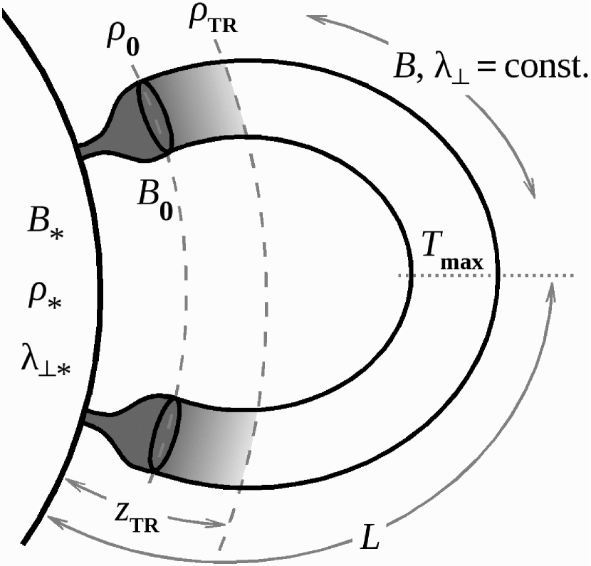
Figure 7.— Simplified portrayal of the assumed coronal loop geometry. Quantities at the photosphere are labeled with subscript $\ast$. Quantities at the flux-tube merging height have subscript 0. Quantities at the transition region have subscript TR. For the T Tauri stars modeled in this paper the photosphere and merging height are identical to one another, and thus the “trumpet” shaped regions between the photosphere and merging height do not occur. Magnetic field $B$ and turbulence correlation length $\lambda_{\perp}$ are assumed to be constant everywhere above the merging height. The rapid drop in density from the merging height to the TR is illustrated by a gradient in grayscale shading.

Figure 7 illustrates the adopted geometry for a representative coronal loop and defines the plasma properties at several key heights. The photospheric values of the magnetic field $B_{\ast}$, density $\rho_{\ast}$, and turbulence correlation length $\lambda_{\perp\ast}$ (see below) are considered to be known for each star. In general, the photospheric magnetic field is fragmented into small flux concentrations surrounded by regions of much weaker field strength. As height increases, the strong field in the concentrations weakens and the cross-sectional area of the flux tube increases. Eventually the flux tubes widen to the point of merging with their neighbors and the magnetic field from the concentrations fills the entire volume above that height. For the Sun, the filling factor $f_{\ast}$ of strong ($\sim$ 1.5 kG) flux tubes in the photosphere ranges between about 0.001 and 0.1, depending on the region. The “merging height” where the flux tubes fill the volume on the Sun tends to occur in the low chromosphere (Cranmer & van Ballegooijen 2005). However, for T Tauri stars with saturated magnetic activity, we will assume $f_{\ast}=1$ (see Saar 2001), and thus the merging height is assumed to be identical to the photosphere.

In Figure 7, the plasma properties at the merging height are labeled with subscript 0. Above the merging height, the closed magnetic flux tubes that fill the corona are modeled as semicircular (i.e., half-torus) loops with constant poloidal radius $r_{\perp}$ and half-length $L$. The conservation of magnetic flux ($\nabla\cdot{\bf B}=0$) thus demands that the magnetic field strength $B_{0}$ is constant along each loop. Observed solar loops tend to have such a constant cross section, but this may be related to their internal structure as collections of thinner twisted strands (e.g., Klimchuk 2006). The sharp transition region (TR) between the cool chromosphere and the hot corona occurs above the merging height. As far as the coronal loop models are concerned, the TR is the effective lower boundary condition. The temperature at the base of the TR is assumed to be a constant value of $10^{4}$ K, and the density and pressure at that location are outputs of the coronal heating model.

This paper uses a general phenomenological expression for the coronal heating rate that was derived from analytic and numerical studies of MHD turbulence. The basic idea is that the photospheric waves (which are produced by both internal convection and the accretion impacts) cause a random shuffling of the magnetic field lines that thread the surface. Magnetic energy in the field is increased via the twisting, shear, and braiding of the field lines (e.g., Parker 1972). Treating this transport and dissipation of magnetic energy as a type of “turbulent cascade” has been found to be useful in parameterizing the eventual coronal heating (van Ballegooijen 1986; Galsgaard & Nordlund 1996; Gómez et al.  2000; Rappazzo et al.  2008). The expression for the volumetric heating rate is

$$Q\,=\,\frac{\rho v_{\perp}^{3}}{\lambda_{\perp}}\left(\frac{\lambda_{\perp}V_{\rm A}}{v_{\perp}L}\right)^{\alpha}$$ (22)

where $\lambda_{\perp}$ is a transverse length scale that represents an effective correlation length for the largest eddies in the turbulent cascade (see also Hollweg 1986; Chae et al.  1998; Cranmer et al.  2007). The turbulent eddies are treated as Alfvén waves that counterpropagate along the loops with equal (i.e., “balanced”) amplitudes in the two directions along the field. Specifically, the Alfvén wave velocity amplitude $v_{\perp}$ and the correlation length $\lambda_{\perp}$ are taken at the merging-height footpoints of the flux tubes. The density $\rho$ and Alfvén speed $V_{\rm A}$ vary with position along the loops.

The magnitude of the Alfvén wave activity on the surface must be modified from the values given by equation (10). That expression gives the photospheric wave amplitude at the poles, but here we need to evaluate the amplitude averaged over the equatorial band of closed magnetic fields. The same numerical code described in Section 4 was used to compute a correction factor that takes account of this geometrical effect. The dimensionless $C_{\rm equ}$ factor is defined similarly to $C_{\rm pol}$ (equation [12]), but the integration is taken from $\theta_{\rm in}$ to the equator ($\theta=\pi/2$), and it is normalized by $\delta_{\rm equ}$. Figure 4 shows how $C_{\rm equ}$ varies as a function of the mean latitude of the accretion streams. In contrast to $C_{\rm pol}$, which always is larger than one, $C_{\rm equ}$ may be less than or greater than one. When the accretion rings are near the poles, the wave power that reaches the pole can be much larger than the average taken over the (large) equatorial band. However, when the accretion rings are near the equator, the wave power that reaches the pole is significantly diminished below that which remains near the equator.

Some additional comments on the form of equation (22) are necessary. The first part of the heating rate ($\rho v_{\perp}^{3}/\lambda_{\perp}$) is a cascade energy flux that is identical to that derived by von Kármán & Howarth (1938) and Kolmogorov (1941) for hydrodynamic turbulence. There may be an order-unity constant that multiplies this quantity (see, e.g., Hossain et al.  1995; Pearson et al.  2004), but this is neglected here for simplicity. The quantity in parentheses in equation (22) is a ratio of the cascade timescale $\tau_{c}=\lambda_{\perp}/v_{\perp}$ to the Alfvén wave transit time along the loop $\tau_{\rm A}=L/V_{\rm A}$. This factor is a uniquely MHD phenomenon and does not appear in hydrodynamic turbulence. When the wave transit time is faster than the cascade time, the nonlinear interactions between turbulent eddies become more infrequent because “wave packets” do not spend as much time interacting with one another (Kraichnan 1965). Thus, the process of building up a power-law spectrum of eddy scales is less efficient when $\tau_{\rm A}\ll\tau_{c}$. In open flux tubes, this gives rise to an overall reduction of the heating rate because the waves/eddies can escape easily. However, in closed-field regions, the waves bounce back and forth between the two ends of the loop and do not escape. A lowering of the cascade efficiency leads to a slower buildup of the turbulent magnetic energy. This longer buildup eventually provides a larger output of heat than would be the case with just the von Kármán term (see, e.g., van Ballegooijen 1986).

The exponent $\alpha$ in equation (22) describes the effectively subdiffusive nature of the cascade in a coronal plasma. The wave-packet interactions discussed above are somewhat muted by various MHD effects such as scale-dependent dynamic alignment (Boldyrev 2005), and these nonlinearities modify the efficiency of the coupling between eddies. The case $\alpha=0$ corresponds to pure hydrodynamic turbulence. Phenomenological expressions used for open field lines in the solar wind (e.g., Oughton et al.  2006; Cranmer et al.  2007) correspond to $\alpha=-1$ in the limit of $\tau_{\rm A}\ll\tau_{c}$. For coronal loops, various models of MHD turbulence have found $\alpha=1.5$ (Gómez et al.  2000), $\alpha=2$ (van Ballegooijen 1986; van Ballegooijen & Cranmer 2008), as well as a continuum of values between 1.5 and 2 that depends on the Alfvén speed and the wave amplitude (Rappazzo et al.  2007, 2008). In this paper we explore only this latter range of values ($1.5\leq\alpha\leq 2$) as being appropriate for closed magnetic loops energized by stellar turbulence.

6.2. Results for Empirical Loop Distributions

For each of the 28 stellar data points from Table 1, we created a distribution of 100 loop lengths that spans the full range of possible values for $L$. The absolute minimum value $L_{\rm min}$ is defined geometrically as the smallest possible toroidal radius at which the “hole” in the torus shrinks to zero size (i.e., $L_{\rm min}=\pi r_{\perp}/2$). To estimate the poloidal radius $r_{\perp}$, it is assumed that both horizontal length scales in the photosphere ($r_{\perp}$ and $\lambda_{\perp}$) are proportional to the photospheric scale height (see, e.g., Robinson et al.  2004). Estimated solar values for $r_{\perp}=200$ km and $\lambda_{\perp}=75$ km (Cranmer et al.  2007) are scaled linearly with the ratio of the stellar to solar values of $H_{\ast}$. The maximum value for the loop length is assumed to reach up to the inner edge of the accretion disk; i.e., $L_{\rm max}=r_{\rm in}-R_{\ast}$.

It should be noted that the precise definitions of the above limits $L_{\rm min}$ and $L_{\rm max}$ are relatively unimportant. We found that the smallest loops in this distribution are likely to be “submerged” below the transition region, and thus they would neither be heated to coronal temperatures nor contribute to the X-ray emission. Also, the largest loops are expected to appear so infrequently that they should not contribute significantly to the disk-averaged X-ray emission (see below). Determining the effective lower limit length for which loops are submerged in the chromosphere is done approximately by first ignoring all loops with $L<z_{\rm TR}$. The height of the transition region is estimated via hydrostatic equilibrium,

$$z_{\rm TR}\,\approx\,H_{\rm eff}\,\ln\left(\rho_{0}/\rho_{\rm TR}\right)\,\,,$$ (23)

and the effective scale height $H_{\rm eff}$ takes account of both gas pressure and wave pressure support: $H_{\rm eff}=(c_{s}^{2}+v_{\perp\ast}^{2})/\gamma g$. For loops with $L>z_{\rm TR}$, we take account of partial submerging by multiplying the expected X-ray fluxes by the quantity $(1-z_{\rm TR}/L)$. For each stellar case in which the shortest loops are canceled out, the minimum loop length $L_{\rm min}$ is redefined as $z_{\rm TR}$.

In some models of T Tauri star coronal heating (e.g., Ryan et al.  2005; Jardine et al.  2006), the longest loops are often modeled as being unstable to “breaking open” into the stellar wind. In many of these models, the gas pressure in loops increases with increasing loop length $L$, and thus the longest loops may have an internal gas pressure that exceeds the surrounding magnetic pressure. However, as described below, the use of equation (22) for the heating rate gives rise to an inverse dependence between loop gas pressure and loop length. The shortest loops are thus the ones most liable to have gas pressure exceed magnetic pressure, but in the present models this does not occur.

The probability distribution $N(L)$ of loop lengths across the stellar surface is assumed to be a power-law function of loop length, with $N(L)\propto L^{-\varepsilon}$ and a sharp cutoff below $L_{\rm min}$. Various solar measurements have constrained the value of the exponent $\varepsilon$ to be approximately 2.5 (Aschwanden et al.  2000, 2008; Close et al.  2003). The models below use $\varepsilon=2.5$ as a fiducial baseline, but they also vary it as a free parameter to evaluate the sensitivity to this assumption. The distribution is normalized such that the equatorial band of closed magnetic field is completely covered by loops. The total surface area available for loops is assumed to be given by $4\pi\delta_{\rm equ}R_{\ast}^{2}$.

For a power-law number distribution of loop lengths, the largest loops (at the upper end of the distribution) do not contribute strongly to any star-averaged quantities. The most probable value of the loop length found on the surface can be estimated from the first moment of the distribution,

$$\langle L\rangle\,=\,\frac{\int dL\,\,N(L)\,\,L}{\int dL\,\,N(L)}$$ (24)

and for a power-law distribution with a sharp cutoff below $L_{\rm min}$, the most probable loop length is $\langle L\rangle=L_{\rm min}(\varepsilon-1)/(\varepsilon-2)$. For $\varepsilon=2.5$, $\langle L\rangle=3L_{\rm min}$. Since we find that $L_{\rm max}$ is typically a factor of 10²–10⁴ larger than $L_{\rm min}$, it is clear that the shortest loops tend to dominate any observable star-averaged properties of the corona. Table 2 gives the most probable loop lengths for all 28 stellar cases.

For a given loop length $L$ and an assumed value of the $\alpha$ exponent in equation (22), it is possible to solve for the temperature and density along each loop. The formulae of Martens (2008) were found to provide the most general way of taking account of a heating rate that depends on the spatially varying plasma properties. Because $V_{\rm A}\propto\rho^{-1/2}$, there is an overall density dependence of the heating rate, with $Q\propto\rho^{1-\alpha/2}$. When $\alpha=2$ the heating rate is constant along the loop, but when $\alpha<2$ the heating is concentrated at the higher-density footpoints. Using the parameterization of Martens (2008), this proportionality is described as $Q\propto P^{1-\alpha/2}/T^{1-\alpha/2}$. Equations (28)–(30) of Martens (2008) then provide solutions for the peak temperature $T_{\rm max}$ and the pressure $P_{\rm TR}$ at the base of the transition region. Neither the density $\rho_{\rm TR}$ nor the Alfvén speed $V_{\rm A,TR}$ at the base of the transition region are known at the outset, but they need to be specified in equation (22) in order to determine the heating rate. Thus, the numerical code used to compute these properties iterates to consistency on $\rho_{\rm TR}$ and $V_{\rm A,TR}$ from an initial estimate.

Because of the large scale heights associated with a hot corona, the loop models have been constructed under the assumption that gas pressure remains constant along the length of each loop (see, however, Serio et al.  1981; Aschwanden & Schrijver 2002). Equation (25) of Martens (2008) is solved for $T(z)$ along the loop, and the constraint of constant pressure provides the density profile $\rho(z)=n(z)m_{\rm H}$. Figure 8 shows an example of the temperatures and number densities along a loop having the most probable length $\langle L\rangle$. As in Figure 6, this plot shows the coronal properties for the HCGD values of AA Tau. The loop geometry has been “unfolded” in Figure 8 such that the two photospheric endpoints occur at $z=0$ and $z=2L$. All plasma quantities were computed between the transition region height $z_{\rm TR}$ and the loop apex ($z=L$), and we assumed symmetry such that both sides of the loop have equal properties.

Figure 8.— Temperature (solid line) and number density (dashed line) plotted as a function of position along a representative coronal loop. Distance is shown in units of the half-length $L$, which for this example is the most-probable length $\langle L\rangle=18.6$ Mm for the HCGD values of AA Tau. This model utilized the iterated coronal heating exponent $\alpha_{\rm R}=1.98$ (see Table 2).

In addition to computing model coronal loops for constant values of $\alpha$, another set of models was constructed with a parameter-dependent choice for $\alpha$ inspired by the results of Rappazzo et al.  (2008). In a set of numerical MHD turbulence simulations for solar coronal loops, Rappazzo et al.  (2008) found that $\alpha$ should depend on the ratio $\cal R$ of the footpoint turbulence amplitude to the coronal Alfvén velocity. Using the definition of the $\alpha$ exponent from equation (22), their numerical results have been fit with the following approximate relation,

$$\alpha_{\rm R}\,\approx\,\frac{2+420{\cal R}}{1+280{\cal R}}$$ (25)

where ${\cal R}=v_{\perp 0}/V_{\rm A,TR}$ and we use the variable name $\alpha_{\rm R}$ to refer specifically to the iterated model value given by equation (25). It is important to note that the exponent $\alpha$ that is defined here differs from the similarly named exponent used by Rappazzo et al.  (2008). If the latter is renamed $\beta$, then $\alpha=(2\beta+3)/(\beta+2)$, and the direct fit of the Rappazzo et al.  (2008) results yielded $\beta_{\rm R}\approx(140{\cal R})^{-1}$. In any case, equation (25) spans a range of possible values between 1.5 and 2. In the loop models computed for this paper, the ratio ${\cal R}$ spans several orders of magnitude between about 10^-5 and 10^-2. Since there are 28 stellar cases and 100 possible loop lengths for each case, there were eventually 2800 individual values of the “preferred” $\alpha_{\rm R}$ exponent. For this large set of values, the mean value of $\alpha_{\rm R}$ was found to be 1.868, with a standard deviation of 0.101 about that mean. For a given star, as $L$ increases so does $\alpha_{\rm R}$.

Table 2 shows example solutions for $T_{\rm max}$, $\alpha_{\rm R}$, the basal number density $n_{\rm TR}=\rho_{\rm TR}/m_{\rm H}$, and the number density at the peak of the loop $n_{\rm top}$. These models are shown for the preferred case of $\alpha=\alpha_{\rm R}$ and for the most probable loop lengths $\langle L\rangle$ as defined above. It is evident that the loop heating rate given by equation (22) provides hot coronal emission with peak temperatures of order 5–10 MK at densities around 10¹⁰ cm^-3. Figure 9 also shows how $T_{\rm max}$ and $n_{\rm top}$ vary as a function of loop length and $\alpha$ for an example stellar case (the HEG values of GM Aur). There is generally more coronal heating for larger values of the $\alpha$ exponent.

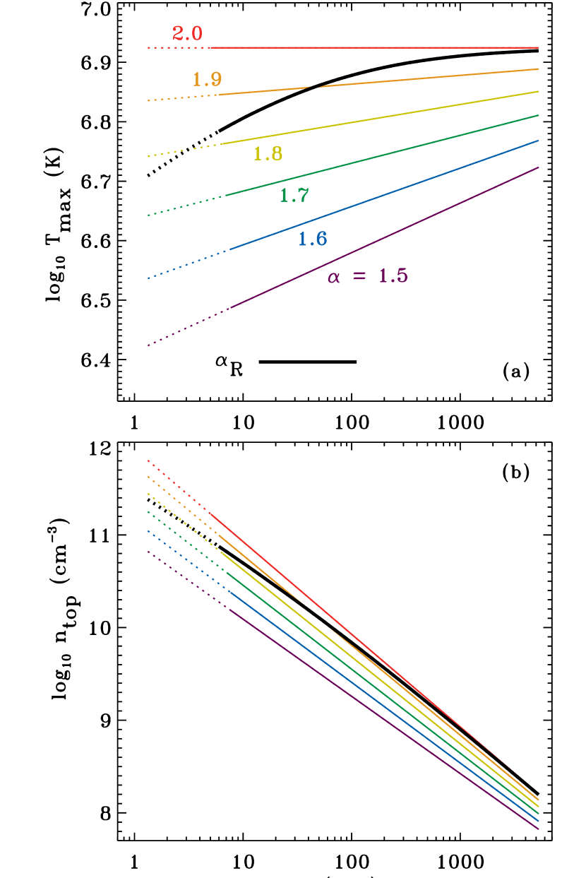
Figure 9.— Parametric plots of (a) loop-top temperature $T_{\rm max}$ and (b) loop-top number density $n_{\rm top}$ versus loop length $L$. Results are shown for a range of possible values of the coronal heating exponent $\alpha$ for an example stellar case (the HCGD values for GM Aur). Colors and labels show results computed for specific constant values of $\alpha$, and the thick black curve denotes models created with the iterated values of $\alpha_{\rm R}$ from equation (25). Dotted portions of each curve denote loops submerged below the TR, which are assumed not to contribute to X-ray emission.

The variation of the coronal heating properties with loop length $L$ seen in Figure 9 can be understood from the basic scaling relations of Martens (2008). Once the parameter dependence of the heating rate is taken into account, the loop-top temperature varies as $T_{\rm max}\propto L^{(2-\alpha)/(3+2\alpha)}$. This exponent varies from 1/12 (for $\alpha=1.5$) to zero (for $\alpha=2$). This scaling is less sensitive to loop length than the classical proportionality derived by Rosner et al.  (1978) for a constant heating rate ($T_{\rm max}\propto L^{4/7}Q^{2/7}$). The basal loop pressure scales as $P_{\rm TR}\propto L^{(3-5\alpha)/(3+2\alpha)}$, and the exponent varies between –3/4 and –1 for the allowed range of $\alpha$ values. In this case, the scaling with loop length is in the opposite sense as Rosner et al.  (1978), who found that $P_{\rm TR}\propto L^{5/7}Q^{6/7}$ for a constant $Q$. For the turbulent heating models of this paper, the fact that $P_{\rm TR}$ decreases with increasing $L$ means that the shortest loops are the ones most in danger of having their gas pressure exceed their magnetic pressure. For the 28 stellar cases, though, the ratio of gas pressure to magnetic pressure (for the shortest coronal loops in each case) ranges from about $10^{-4}$ to $10^{-2}$. Thus, the equatorial coronal loops modeled here do not appear to be unstable to breaking open into a stellar wind.

Finally, it is useful to confirm the validity of the adopted heating rate and loop modeling procedure by applying representative values for well-observed solar loops. The Sun’s photospheric filling factor for strong-field magnetic flux tubes is much smaller than unity. Here we assume $f_{\ast}=0.05$, which is consistent with a mean field strength at the merging height of about 70 G. This corresponds to a weak active region or small sunspot. At the merging height, the transverse footpoint velocity amplitude $v_{\perp}\approx 1$ km s^-1, and the correlation length $\lambda_{\perp}\approx 350$ km. Taking the typical value $\alpha=1.9$ for a representative loop with $L=50$ Mm, the iteration process described above gives rise to realistic values for the basal Alfvén speed $V_{\rm A,TR}\approx 900$ km s^-1, the transition region number density $n_{\rm TR}\approx 3\times 10^{10}$ cm^-3, and the peak temperature $T_{\rm max}\approx 1.2$ MK. The temperature is slightly on the low side for an active region, but it is consistent with much of the fine loop structure observed in the extreme UV by TRACE (Lenz et al.  1999; Aschwanden 2006). Applying a loop length distribution with $\varepsilon=2.5$ and computing the surface average of the energy flux ($F\sim QL$), this solar model gives a mean value of $5\times 10^{6}$ erg cm^-2 s^-1. This is in the middle of the empirically allowed range for active region loops (e.g., Withbroe & Noyes 1977).

7. X-Ray Luminosities

The accretion shocks (Section 5) and coronal loops (Section 6) are both expected to give rise to significant X-ray emission. Their total X-ray luminosities $L_{\rm X}$ are estimated here and compared with existing observations. The calculations of X-ray flux are done under the optically thin assumption that all radiation escapes from the emitting regions. The absorption by intervening material is not taken into account because that has been shown to be sensitively dependent on both the assumed magnetic geometry and the observer’s orientation (e.g., Gregory et al.  2007). Future work should include these effects and compute time-dependent X-ray light curves for observers at a range of inclinations.

The emissivity of each volume element of plasma was treated using version 5.2.1 of the CHIANTI atomic database (Dere et al.  1997; Landi et al.  2006). The models used a standard solar abundance mixture (Grevesse & Sauval 1998) and collisional ionization balance (Mazzotta et al.  1998) to compute the emissivity as a function of wavelength over the X-ray bandpasses of interest. This provided a bandpass-dependent radiative loss rate ($Q_{\rm X}=n_{e}^{2}\Lambda_{\rm X}(T)$) that was then used to sum up the contributions of the emitting volume elements. For structures near the surfaces of the stars, it is valid to estimate the X-ray luminosity as

$$L_{\rm X}\,=\,4\pi\delta R_{\ast}^{2}\int dz\,\,[n_{e}(z)]^{2}\Lambda_{\rm X}[T(z)]\,\,,$$ (26)

where the fraction $\delta$ is used for the accretion shock regions and it is replaced by $\delta_{\rm equ}$ for the equatorial coronal loop regions.

Figure 10.— (a) Normalized X-ray efficiencies for the ROSAT PSPC (dashed line) and for the medium thickness filter on XMM-Newton’s EPIC-pn camera (solid line). (b) Temperature dependence of optically thin radiative loss functions computed for the ROSAT bandpass (dashed line), the XMM bandpass (solid line), and for all photons (dotted line).

Figure 10 shows the relevant X-ray response functions and their associated radiative loss rates. Two observational bandpasses are discussed in this paper. The first is that of the ROSAT Position Sensitive Proportional Counter (PSPC), with the X-ray efficiency function specified by Judge et al.  (2003). The sensitivity is nonzero between about 0.1 and 2.4 keV, with a minimum around 0.3 keV that separates the hard and soft bands. The second bandpass shown is that of the XMM-Newton European Photon Imaging Camera (EPIC), and Figure 10(a) shows the sensitivity function for the medium thickness filter on the EPIC-pn camera (e.g., Dahlem & Schartel 1999; Strüder et al.  2001). Figure 10(b) shows the result of folding the optically thin emissivities computed with CHIANTI through the two response functions, as well as the full radiative loss curve that includes photons of all wavelengths (see, e.g., Raymond et al.  1976; Schmutzler & Tscharnuter 1993).

Table 3Observed and Modeled X-ray Luminosities

	Observed			Modeled
				Shocks	Shocks	Loops, $\alpha=1.5$	Loops, $\alpha=2$	Loops, $\alpha=\alpha_{\rm R}$	Loops, $\alpha=\alpha_{\rm R}$
Object	ROSAT	XMM		(ROSAT)	(XMM)	(ROSAT)	(ROSAT)	(ROSAT)	(XMM)
AA Tau	29.642	30.094		26.775	26.094	29.071	30.777	29.871	30.013
	29.642	30.094		29.579	28.962	26.231	29.254	29.100	29.249
BP Tau	29.849	30.135		25.488	24.838	26.031	28.344	27.999	28.132
	29.849	30.135		29.465	28.760	25.615	28.211	28.000	28.144
CY Tau	$<$29.797	29.288		30.693	30.462	27.857	29.833	29.120	29.266
	$<$29.797	29.288		30.257	29.750	25.972	28.710	28.513	28.663
DE Tau	$<$29.458	…		26.936	26.265	29.856	31.672	30.734	30.908
	$<$29.458	…		28.966	28.262	27.498	30.444	30.218	30.371
DF Tau	29.810	…		28.096	27.405	28.784	30.958	30.248	30.396
	29.810	…		29.243	28.532	28.539	30.814	30.157	30.302
DK Tau	$<$29.348	29.962		…	…	28.407	30.458	29.689	29.835
	$<$29.348	29.962		25.635	24.982	25.960	28.995	28.863	29.011
DN Tau	29.751	30.063		27.942	27.221	28.637	30.447	29.606	29.750
	29.751	30.063		28.098	27.395	27.205	29.860	29.505	29.652
DO Tau	$<$29.316	…		26.033	25.368	28.119	30.093	29.348	29.493
	$<$29.316	…		30.596	29.889	27.562	29.706	29.050	29.195
DS Tau	$<$29.877	…		23.213	22.477	29.394	31.136	30.248	30.393
	$<$29.877	…		30.394	29.852	28.306	30.449	29.612	29.766
GG Tau	$<$29.029	…		25.730	25.081	29.060	30.629	29.650	29.798
	$<$29.029	…		30.075	29.405	26.708	29.313	28.956	29.099
GI Tau	29.382	29.921		26.491	25.827	28.820	30.641	29.814	29.958
	29.382	29.921		29.523	28.819	28.597	30.682	29.976	30.120
GM Aur	29.750	…		17.593	16.452	28.633	30.490	29.609	29.754
	29.750	…		24.557	23.908	28.518	30.500	29.674	29.822
HN Tau	$<$29.709	…		31.208	30.986	28.751	30.609	29.605	29.748
	$<$29.709	…		30.790	30.921	28.757	30.626	29.673	29.816
UY Aur	$<$29.403	…		25.957	25.307	28.119	30.323	29.524	29.669
	$<$29.403	…		29.688	28.985	27.825	30.097	29.461	29.608

Table 3 lists the observed and predicted X-ray luminosities for a variety of cases. The ROSAT observations were taken from Neuhäuser et al.  (1995). Two of the measurements listed under the ROSAT column (for DF Tau and GM Aur) were made with the Einstein Imaging Proportional Counter (IPC) which has a similar X-ray bandpass as the ROSAT PSPC (Damiani et al.  1995). The XMM-Newton measurements were reported by Güdel et al.  (2007a). For the 4 out of 14 stars for which there are firm observations from both telescopes, the ratios of XMM to ROSAT luminosities range between 1.9 and 3.5. The curves in Figure 10(b) show a similar range of enhancement for temperatures between about 20 and 120 MK.

The representative example of a solar coronal loop discussed at the end of Section 6 can be used to help confirm the validity of the theoretical X-ray luminosity estimates. For this example, using the ROSAT bandpass and integrating over the full loop-length distribution yielded $L_{\rm X}=1.5\times 10^{27}$ erg s^-1, or a ratio $L_{\rm X}/L_{\odot}=4\times 10^{-7}$. This is inside the observed range of variability for the Sun (Judge et al.  2003).

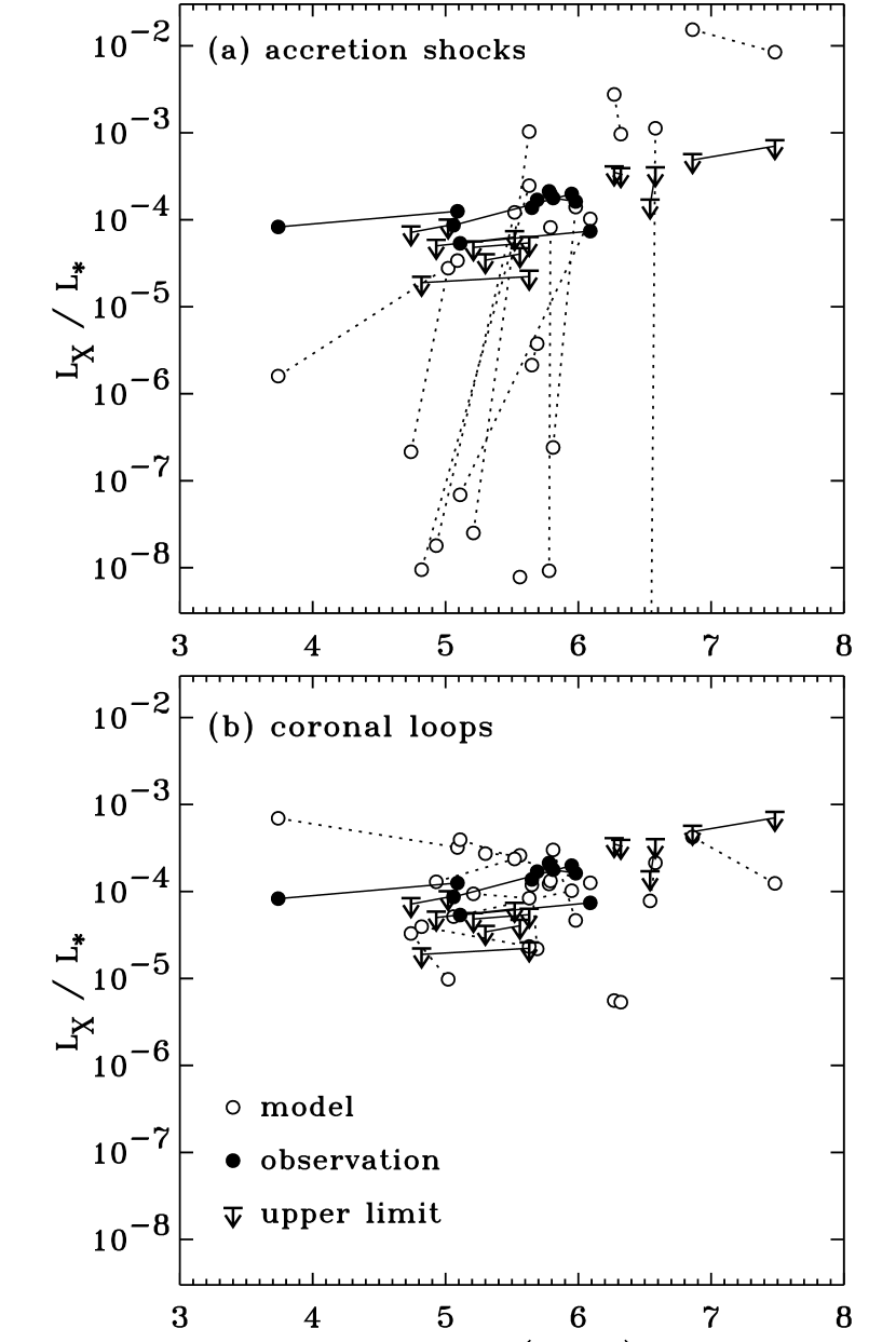
Figure 11.— Individual results for $L_{\rm X}/L_{\ast}$ shown as a function of age, corresponding to (a) the accretion shock models and (b) coronal loop models computed with the optimized $\alpha=\alpha_{\rm R}$ exponents. Model values computed with the ROSAT bandpass (open circles) are compared against direct ROSAT observations (filled circles) and upper limits (downward arrows).

Figure 11 shows the ratios $L_{\rm X}/L_{\ast}$ for the 28 stellar cases, computed using the ROSAT bandpass for both the accretion shock models and a representative set of coronal loop models (i.e., the optimized case of $\alpha=\alpha_{\rm R}$). Table 3 also lists the predicted $L_{\rm X}$ values for these models, as well as the corresponding XMM bandpass luminosities. Loop model results are also given (for the ROSAT bandpass only) for the cases of fixed values of $\alpha=1.5$ and 2. Figure 11(a) shows the modeled X-ray luminosities for the accretion shock models. These values span a much wider range than the observations. The youngest stars that generally have the highest accretion rates (but lowest values of $v_{c}$ and $T_{\rm sh}$) tend to have negligibly small predicted values of $L_{\rm X}$ from the accretion shocks. Figure 11(b) shows the predicted X-ray luminosities from the coronal loops, and these appear to fall more closely within the observed range of values.

Note from Table 3 that the modeled XMM luminosities for the accretion shock models are typically lower than the ROSAT bandpass values. Apart from one outlier (the HCGD value of HN Tau), nearly all of the modeled stellar cases have ratios of XMM to ROSAT $L_{\rm X}$ between 0.07 and 0.6. For the coronal loop models, however, this ratio spans a higher range between about 0.6 and 1.7. The values less than 1 apply only for models that use $\alpha\lesssim 1.6$, and for the optimized models that use $\alpha=\alpha_{\rm R}$ the range of XMM to ROSAT ratios is 1.3 to 1.5. This is consistent with the fact that most of the loop-top temperatures $T_{\rm max}$ are between about 5 and 10 MK (see Figure 10(b)). In any case, these ratios are well below the observed range of 1.9 to 3.5. This may indicate that the present models underestimate the coronal temperatures.

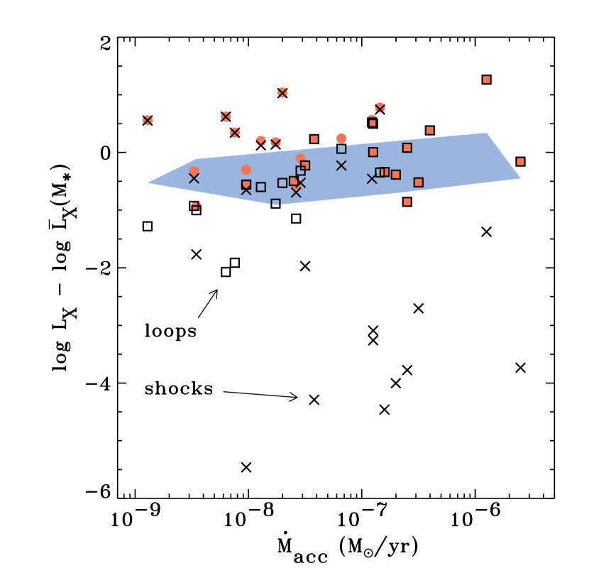
Figure 12.— Residual X-ray luminosity (i.e., deviation of $L_{\rm X}$ from the mean observational trend with stellar mass $\bar{L}_{\rm X}(M_{\ast})$) shown as a function of mass accretion rate. Model results include individual luminosities from the accretion shocks (crosses), the coronal loop models computed with optimized $\alpha_{\rm R}$ (squares), and the sum of these two components (red filled circles). The approximate region subtended by the ROSAT observations is illustrated by a blue polygon.

In order to assess the relative contributions from accretion shocks and coronal loops, Figure 12 shows the modeled X-ray luminosities (again just using the ROSAT bandpass) as a function of the stellar accretion rate. In this plot, we follow Drake et al.  (2009) and plot the residual X-ray luminosity, in which the general trend for higher-mass stars to have a larger $L_{\rm X}$ has been first removed. The mean mass dependence has been taken from the Chandra COUP data sample (Preibisch et al.  2005), with

$$\log\bar{L}_{\rm X}(M_{\ast})\,=\,30.34+1.13\log(M_{\ast}/M_{\odot})\,\,.$$ (27)

Figure 12 shows the individual $L_{\rm X}$ contributions from accretion shocks and coronal loops for each stellar case, as well as their sum. The totals generally fall within the range of observed values (shown as an irregular blue polygon). Of the 28 stellar cases shown in Figure 12, 8 of them have X-ray luminosities that are clearly dominated by the accretion shocks (i.e., they have more than a 75% relative contribution from the shock emission) and 16 are clearly dominated by the coronal loops (with more than a 75% contribution from the loops). The 4 remaining cases have a rough balance between the two components; these correspond to the HCGD values of BP Tau, DE Tau, GI Tau, and UY Aur. Figure 12 shows that, generally, the highest values of $\dot{M}_{\rm acc}$ correspond to the cases dominated by coronal loops. The stars with the lowest accretion rates are the ones with $L_{\rm X}$ dominated by the accretion shocks.

The recent study of Drake et al.  (2009) indicated the existence of an anticorrelation between accretion rate and X-ray luminosity for some T Tauri stars. This appears to be consistent with the well-known trend for WTTS (weak-lined T Tauri stars, which are not accreting) to be more X-ray bright than accreting CTTS (e.g., Neuhäuser et al.  1995; Flaccomio et al.  2003a,b; Telleschi et al.  2007; Briggs et al.  2007). However, neither the observational data nor the model results shown in Figure 12 yield such an anticorrelation. If one examines just the modeled coronal loop $L_{\rm X}$ values, it is clear that there tends to be a positive correlation with accretion rate. This makes sense since the coronal heating is largely driven by MHD turbulence excited in the accretion streams. The X-ray luminosities associated with the accretion shocks are roughly anticorrelated with accretion rate. When the two components are summed, however, these effects largely cancel each other out, and the result is little to no correlation with accretion rate. Of course, the present sample does not span the wider range of ages and accretion rates that one would find when comparing WTTS and CTTS.

Another way to assess the validity of the models is to perform a direct star-by-star $\chi^{2}$ analysis of the differences between the observed and modeled X-ray luminosities. This analysis uses the summed $L_{\rm X}$ from both the accretion shock and coronal loop regions for each stellar case. Also, only the most definitive observations are used. Only the 6 ROSAT observations with firm measurements (e.g., AA Tau, BP Tau, DF Tau, DN Tau, GI Tau, and GM Aur) and the 2 XMM measurements that exist for stars having only ROSAT upper limits (e.g., CY Tau and DK Tau) are used in this analysis. This results in 8 stars (or 16 unique model data points) to compare with the observations. The $\chi^{2}$ statistic computed for a given set of models is defined as

$$\chi^{2}\,=\,\frac{1}{\sigma^{2}}\sum\left(\log L_{\rm X,obs}-\log L_{\rm X,model}\right)^{2}\,\,,$$ (28)

where $\sigma=0.5$ dex was adopted as the logarithm of a representative observational uncertainty (see, e.g., Neuhäuser et al.  1995) and the above sum is taken over the 16 data points. Each term in the sum uses the appropriate bandpass for each of the $L_{\rm X}$ values; i.e., each term compares either ROSAT observations to ROSAT-bandpass models, or XMM observations to XMM-bandpass models.

The $\chi^{2}$ quantity defined in equation (28) constrains the probability that the observed and modeled data sets are in agreement with one another. Assuming normally distributed uncertainties, this probability is given by Press et al.  (1992) as

$$P\,\equiv\,Q(\chi^{2}|\nu)=\frac{1}{\Gamma(\nu/2)}\int_{\chi^{2}/2}^{\infty}e^{-t}t^{(\nu/2)-1}dt\,\,,$$ (29)

where $\nu$ is the effective number of degrees of freedom, which we take as 16 (the number of data points), and $\Gamma(x)$ is the complete Gamma function. When $\chi^{2}\ll\nu$ the above probability approaches unity (i.e., the modeled luminosities are a good match to the observed luminosities), and when $\chi^{2}\gg\nu$ the above probability is negligibly small.

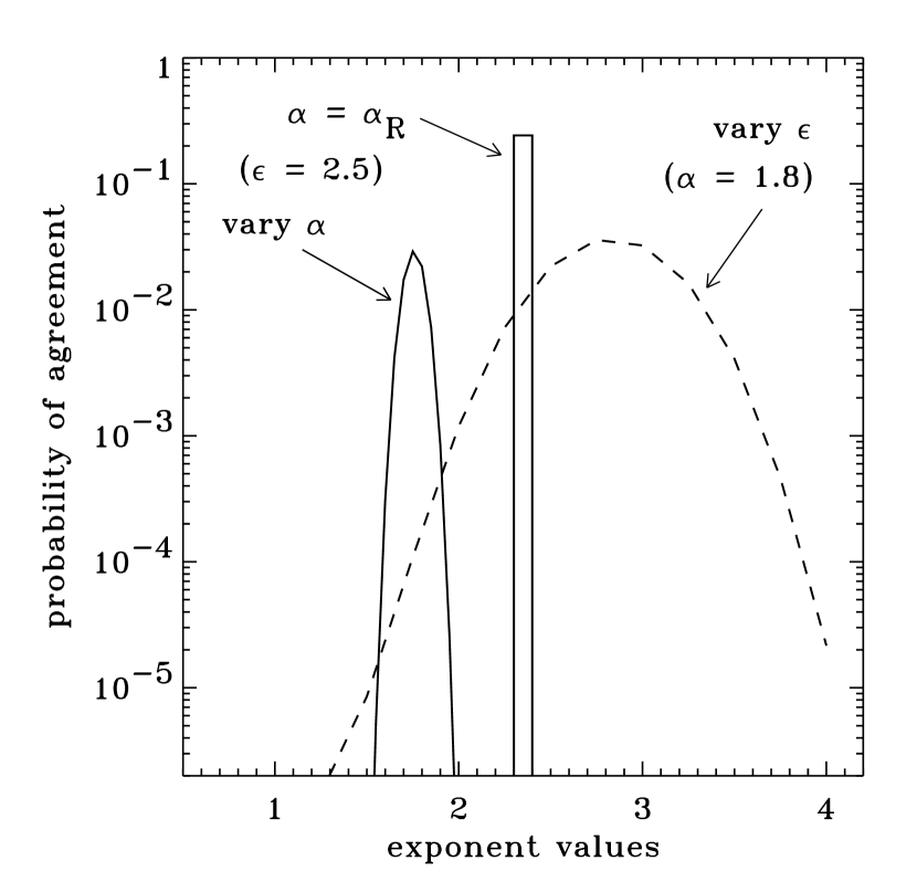
Figure 13.— Computed probabilities of agreement between X-ray observations and the modeled total (shock plus loop) values of $L_{\rm X}$ for a set of 8 well-observed stars. Models are shown that vary the coronal heating exponent $\alpha$ (solid curves) and those that vary the loop number distribution exponent $\varepsilon$ (dashed curve). For clarity, the single histogram corresponding to the optimized $\alpha_{\rm R}$ models is placed to the right of the other models that assume a range of constant $\alpha$ exponents (i.e., the plotted abscissa value for this case was chosen arbitrarily).

Figure 13 shows the results of several calculations of the above probability. Because there were no real free parameters to vary for the accretion shock models, all of the models shown in Figure 13 vary either the coronal-loop heating exponent $\alpha$ or the loop number distribution exponent $\varepsilon$. When $\alpha$ was varied (keeping $\varepsilon$ fixed at its standard value of 2.5), the highest probability of agreement with the observations was clearly found for the optimized case of $\alpha=\alpha_{\rm R}$. This model resulted in a reduced $\chi^{2}/\nu=1.22$, which corresponds to a probability of 24%. For fixed values of $\alpha$, the exponent was varied between 1.5 and 2 with an increment of 0.05. The highest-probability model of these was $\alpha=1.75$, with a reduced $\chi^{2}/\nu$ of 1.77 and a probability of about 3%.

Varying the loop-length number distribution exponent $\varepsilon$ was also done by keeping $\alpha$ fixed at a value of 1.8. As $\varepsilon$ increases, the shortest loops in the distribution are weighted more strongly. Thus, higher values of $\varepsilon$ produce more X-ray emission from cooler and denser regions, and lower values of $\varepsilon$ produce emission from hotter and more tenuous regions. For each star, $L_{\rm X}$ for the entire distribution of loops decreases as $\varepsilon$ increases. Figure 13 shows the resulting probabilities for a grid of models computed for a range of $\varepsilon$ between 1 and 4 with an increment of 0.25. The most successful model of these was for $\varepsilon=2.75$, with only a marginally better probability than for the standard value of 2.5 (i.e., both of these models are near the peak of the probability curve).

Finally, another set of models was computed to address the concerns raised in Section 5 about a possible overestimation of the deceleration experienced by accreting clumps. The postshock temperatures $T_{\rm sh}$ shown in Table 2 are generally lower than the typically reported range of 2–3 MK for CTTS accretion shocks. Thus, it is possible that the clump speed $v_{c}$ has been reduced too much below the ballistic free-fall speed $v_{\rm ff}$ by the effects discussed in Section 3. A set of accretion shock and coronal loop models were thus computed under the assumption that no deceleration occurs (i.e., that $v_{c}=v_{\rm ff}$). The resulting X-ray luminosities from the accretion shock regions were substantially larger than in the standard models, with 11 out of the 28 stellar cases experiencing more than a factor of 100 increase in $L_{\rm X}$ (with 6 of these 11 having more than a factor of $10^{4}$ increase), and only 6 other cases exhibiting no change in $L_{\rm X}$. The photospheric Alfvén wave amplitudes for these models were significantly larger than in the standard models, and thus the coronal-loop heating was larger. Loop models with $\alpha=1.75$ (which is the best-fitting model with constant $\alpha$ in Figure 13) yielded an increase in $L_{\rm X}$ of factors of order 2–6 for 10 of the 28 models and either equal or slightly lower luminosities for 8 of the 28 cases. Summing the shock and loop model luminosities and performing the $\chi^{2}$ comparison with the observations, as described above, yielded a substantially decreased probability of agreement for these “undecelerated” models, with $P=9\times 10^{-5}$ for the case of $\alpha=1.75$ and $\varepsilon=2.5$. This is a reduction in probability from the corresponding standard model (see above) of about a factor of 300. Similar results for other values of $\alpha$ lead to the conclusion that some degree of clump deceleration is necessary for optimal agreement with observed X-rays.

8. Discussion and Conclusions

The primary aim of this paper has been to explore and test a set of physical processes that may be responsible for producing stellar winds and coronal X-ray activity in accreting T Tauri stars. A key new aspect of this work is the self-consistent generation of plasma heating and wind acceleration (via MHD waves and turbulence) for a database of well-observed CTTS in the Taurus-Auriga region. Scheurwater & Kuijpers (1988) and Cranmer (2008) suggested that inhomogeneous accretion can give rise to enhanced MHD wave amplitudes across the stellar surface. In this paper, the consequences of these turbulent motions were studied further and applied to both wave-driven wind models and footpoint-shaking models for coronal loops. By and large, the predicted X-ray luminosities from a combination of accretion shocks and hot loops agrees reasonably well with existing observations. The resulting mass loss rates for polar CTTS winds tend to be lower than those derived from measurements. This indicates that disk winds or X-winds (i.e., outflows not rooted to the stellar surface) may be responsible for many of those measurements. However, in several of the modeled cases the stellar winds do appear to contribute significantly to the measured mass loss rates.

The models presented above have shown that it is plausible to assume that the accretion energy is sufficient to drive CTTS stellar winds and coronal X-ray emission. However, this cannot explain the even stronger X-ray emission from WTTS, which are believed to not be accreting at all. Even if the lower X-ray fluxes of CTTS were the result of absorption in the accretion columns (e.g., Gregory et al.  2007), the relatively unattenuated X-rays of WTTS should not be explainable by accretion-driven phenomena. Here it was assumed that the accretion-driven component of surface MHD turbulence dominates the intrinsic convection-driven component. Young, rapidly rotating stars are suspected of having more vigorous convective motions, higher internal dynamo activity, and more frequent magnetic flux emergence than older stars such as the Sun (e.g., Montalbán et al.  2004; Ballot et al. 2007; Holzwarth 2007; Brown et al.  2008; Käpylä et al.  2009). Rapid rotation can also give rise to complex field-line motions that lead to propeller-driven outflows, collimated jets, or “magnetic towers” (Blandford & Payne 1982; Lynden-Bell 2003; Ustyugova et al.  2006; Romanova et al.  2009). More accurate models must include these kinds of effects.

In this paper, an attempt was made to reduce the number of freely adjustable parameters by as much as possible. For example, although the accretion shock model (Section 5) depends on many assumptions about the magnetic geometry and the form of the radiative cooling function, it does not contain any truly ad hoc free parameters. The coronal loop model (Section 6) utilizes a state-of-the-art parameterization for the heating that comes from MHD turbulent dissipation, and the best value for the $\alpha$ exponent in that parameterization turns out to be one that has been fit from a series of numerical simulations (e.g., equation [25]). However, all of the models presented in this paper do depend on various assumptions that had to be made about the clumpiness of the accreting gas, and about how these clumps may be decelerated as they fall from the inner edge of the disk. Future models of inhomogeneous accretion should focus on improving our understanding of the dynamics of individual clumps.

The use of a rotationally aligned dipole magnetic field in this paper is a shortcoming that should be remedied in future models. In fact, there has been much work done recently to create three-dimensional models of CTTS magnetospheres (e.g., Koldoba et al.  2002; Romanova et al.  2003, 2004, 2008; Gregory et al.  2006, 2009; Long et al.  2007, 2008). Such models can naturally include the effects of X-ray absorption by the accretion columns and the dynamics of disk winds or X-winds. Still, many of these models utilize relatively simple approximations for the conservation of internal energy. Their realism and predictive power could be improved by including the effects of MHD waves and turbulence as described above. Thus, it is possible that the most useful results of this paper may not be the specific model results, but instead the general methodology for wave generation and coronal heating that can be inserted into more advanced simulations.

In addition to improving the physical models of the stellar plasmas, it will also be important to model the emergent radiation more accurately. For X-rays, the simulation of bandpass-integrated luminosities (Section 7) is only the beginning of the story. There is a great deal of diagnostic information in the X-ray spectrum that can be used to constrain the properties of the various plasma components. Recent X-ray spectral analyses are beginning to reveal that there may be other distinct emitting regions in addition to the three studied in this paper (e.g., winds, accretion shocks, and coronal loops). One of these other classes includes transient phenomena such as strong flares, eruptions, and other outcomes of large-scale magnetic reconnection (e.g., Giardino et al.  2006; Kastner et al.  2006; Aarnio et al.  2009). Another newly discovered region appears to be filled with cooler and lower-density coronal plasma than is in the dominant coronal loops (Brickhouse et al.  2009). These regions may be turbulent “boundary layers” that surround the accretion spots and are magnetically connected to both the shocked plasma and the loops (see also Hujeirat & Papaloizou 1998).

I gratefully acknowledge Nancy Brickhouse, Adriaan van Ballegooijen, and Andrea Dupree for many valuable discussions, as well as Sean Matt for helping me discover an error in an earlier version of this paper. This work was supported by the Sprague Fund of the Smithsonian Institution Research Endowment, and by the National Aeronautics and Space Administration (NASA) under grant NNG04GE77G to the Smithsonian Astrophysical Observatory.

References

- (1) Aarnio, A. N., Stassun, K. G., & Matt, S. P. 2009, in AIP Conf. Proc. 1094, 15th Cambridge Workshop on Cool Stars, Stellar Systems, and the Sun, ed. E. Stempels (Melville, NY: AIP), 337
- (2) Airapetian, V. S., Ofman, L., Robinson, R. D., Carpenter, K., & Davila, J. 2000, ApJ, 528, 965
- (3) Argiroffi, C., Maggio, A., & Peres, G. 2007, A&A, 465, L5
- (4) Aschwanden, M. J. 2006, Physics of the Solar Corona: An Introduction with Problems and Solutions, 2nd ed. (Berlin: Springer)
- (5) Aschwanden, M. J., Lee, J. K., Gary, G. A., Smith, M., & Inhester, B. 2008, Sol. Phys., 248, 359
- (6) Aschwanden, M. J., & Schrijver, C. J. 2002, ApJS, 142, 269
- (7) Aschwanden, M. J., Tarbell, T. D., Nightingale, R. W., Schrijver, C. J., Title, A., Kankelborg, C. C., Martens, P., & Warren, H. P. 2000, ApJ, 535, 1047
- (8) Azevedo, R., Folha, D. F. M., Gameiro, J. F., & Calvet, N. 2007, ApJ, 670, 1234
- (9) Ballot, J., Brun, A. S., & Turck-Chièze, S. 2007, ApJ, 669, 1190
- (10) Baraffe, I., Chabrier, G., & Gallardo, J. 2009, ApJ, 702, L27
- (11) Batalha, C., Batalha, N. M., Alencar, S. H. P., Lopes, D. F., & Duarte, E. S. 2002, ApJ, 580, 343
- (12) Blandford, R. D., & Payne, D. G. 1982, MNRAS, 199, 883
- (13) Boldyrev, S. 2005, ApJ, 626, L37
- (14) Bouvier, J., Dougados, C., & Alencar, S. H. P. 2004, Ap&SS, 292, 659
- (15) Bouvier, J., et al. 2003, A&A, 409, 169
- (16) Bouvier, J., et al. 2007, A&A, 463, 1017
- (17) Brickhouse, N. S., Cranmer, S. R., Dupree, A. K., Luna, G. J. M., & Wolk, S. J. 2009, ApJ, submitted
- (18) Briggs, K. R., et al. 2007, A&A, 468, 413
- (19) Brown, B. P., Browning, M. K., Brun, A. S., Miesch, M. S., & Toomre, J. 2008, ApJ, 689, 1354
- (20) Calvet, N. 1997, in IAU Symp. 182, Herbig-Haro Flows and the Birth of Stars, ed. B. Reipurth & C. Bertout (Dordrecht: Kluwer), 417
- (21) Calvet, N., Muzerolle, J., Briceño, C., Hernández, J., Hartmann, L., Saucedo, J. L., & Gordon, K. D. 2004, AJ, 128, 1294
- (22) Calvet, N., & Gullbring, E. 1998, ApJ, 509, 802
- (23) Calvet, N., & Hartmann, L. 1992, ApJ, 386, 239
- (24) Camenzind, M. 1990, Rev. Mod. Astron., 3, 234
- (25) Casse, F., Meliani, Z., & Sauty, C. 2007, Ap&SS, 311, 57
- (26) Chae, J., Schühle, U., & Lemaire, P. 1998, ApJ, 505, 957
- (27) Chevalier, R. A., & Imamura, J. N. 1982, ApJ, 261, 543
- (28) Close, R. M., Parnell, C. E., Mackay, D. H., & Priest, E. R. 2003, Sol. Phys., 212, 251
- (29) Costa, V. M., Lago, M. T. V. T., Norci, L., & Meurs, E. J. A. 2000, A&A, 354, 621
- (30) Cranmer, S. R. 2002, Space Sci. Rev., 101, 229
- (31) Cranmer, S. R. 2008, ApJ, 689, 316
- (32) Cranmer, S. R. 2009, Living Rev. Solar Phys., 6, lrsp-2009-3
- (33) Cranmer, S. R., & van Ballegooijen, A. A. 2005, ApJS, 156, 265
- (34) Cranmer, S. R., van Ballegooijen, A. A., & Edgar, R. J. 2007, ApJS, 171, 520
- (35) D’Antona, F., & Mazzitelli, I. 1994, ApJS, 90, 467
- (36) Dahlem, M., & Schartel, N. 1999, XMM Users’ Handbook, Issue 1.1 (Noordwijk, The Netherlands: ESA)
- (37) Damiani, F., Micela, G., Sciortino, S., & Harnden, F. R., Jr. 1995, ApJ, 446, 331
- (38) DeCampli, W. M. 1981, ApJ, 244, 124
- (39) Dere, K. P., Landi, E., Mason, H. E., Monsignori Fossi, B. C., & Young, P. R. 1997, A&AS, 125, 149
- (40) Donati, J.-F., et al. 2007, MNRAS, 380, 1297
- (41) Drake, J. J., Ercolano, B., Flaccomio, E., & Micela, G. 2009, ApJ, 699, L35
- (42) Edwards, S. 2009, in AIP Conf. Proc. 1094, 15th Cambridge Workshop on Cool Stars, Stellar Systems, and the Sun, ed. E. Stempels (Melville, NY: AIP), 29
- (43) Elmegreen, B. G. 1990, ApJ, 361, L77
- (44) Falceta-Gonçalves, D., Vidotto, A. A., & Jatenco-Pereira, V. 2006, MNRAS, 368, 1145
- (45) Feigelson, E. D., & Montmerle, T. 1999, ARA&A, 37, 363
- (46) Feldmeier, A., Kudritzki, R.-P., Palsa, R., Pauldrach, A. W. A., & Puls, J. 1997, A&A, 320, 899
- (47) Fendt, C. 2009, ApJ, 692, 346
- (48) Ferguson, J. W., Alexander, D. R., Allard, F., Barman, T., Bodnarik, J. G., Hauschildt, P. H., Heffner-Wong, A., & Tamanai, A. 2005, ApJ, 623, 585
- (49) Ferreira, J., Dougados, C., & Cabrit, S. 2006, A&A, 453, 785
- (50) Flaccomio, E., Micela, G., & Sciortino, S. 2003a, A&A, 397, 611
- (51) Flaccomio, E., Micela, G., & Sciortino, S. 2003b, A&A, 402, 277
- (52) Galsgaard, K., & Nordlund, Å. 1996, J. Geophys. Res., 101, 13445
- (53) Giardino, G., Favata, F., Pillitteri, I., Flaccomio, E., Micela, G., & Sciortino, S. 2007, A&A, 475, 891
- (54) Giardino, G., Favata, F., Silva, B., Micela, G., Reale, F., & Sciortino, S. 2006, A&A, 453, 241
- (55) Gómez, D. O., Dmitruk, P. A., & Milano, L. J. 2000, Sol. Phys., 195, 299
- (56) Gómez de Castro, A. I., & Verdugo, E. 2007, ApJ, 654, L91
- (57) Gregory, S. G., Flaccomio, E., Argiroffi, C., Bouvier, J., Donati, J. -F., Feigelson, E. D., Getman, K. V., Hussain, G. A. J., Jardine, M., & Walter, F. M. 2009, preprint, arXiv:0906.4880
- (58) Gregory, S. G., Jardine, M., Collier Cameron, A., & Donati, J.-F. 2006, MNRAS, 373, 827
- (59) Gregory, S. G., Matt, S. P., Donati, J.-F., & Jardine, M. 2008, MNRAS, 389, 1839
- (60) Gregory, S. G., Wood, K., & Jardine, M. 2007, MNRAS, 379, L35
- (61) Grevesse, N., & Sauval, A. J. 1998, Space Sci. Rev., 85, 161
- (62) Grosso, N., Bouvier, J., Montmerle, T., Fernández, M., Grankin, K., & Zapatero Osorio, M. R. 2007, A&A, 475, 607
- (63) Güdel, M., et al. 2007a, A&A, 468, 353
- (64) Güdel, M., Telleschi, A., Audard, M., Skinner, S. L., Briggs, K. R., Palla, F., & Dougados, C. 2007b, A&A, 468, 515
- (65) Gullbring, E. 1994, A&A, 287, 131
- (66) Gullbring, E., Barwig, H., Chen, P. S., Gahm, G. F., & Bao, M. X. 1996, A&A, 307, 791
- (67) Gullbring, E., Hartmann, L., Briceño, C., & Calvet, N. 1998, ApJ, 492, 323
- (68) Günther, H. M., Schmitt, J. H. M. M., Robrade, J., & Liefke, C. 2007, A&A, 466, 1111
- (69) Hartigan, P., Edwards, S., & Ghandour, L. 1995, ApJ, 452, 736 (HEG)
- (70) Hartigan, P., Edwards, S., & Pierson, R. 2004, ApJ, 609, 261
- (71) Hartmann, L., Calvet, N., Gullbring, E., & D’Alessio, P. 1998, ApJ, 495, 385 (HCGD)
- (72) Hartmann, L., Cassen, P., & Kenyon, S. J. 1997, ApJ, 475, 770
- (73) Hartmann, L., & MacGregor, K. B. 1980, ApJ, 242, 260
- (74) Hartmann, L., & Noyes, R. W. 1987, ARA&A, 25, 271
- (75) Hollweg, J. V. 1978, Rev. Geophys. Space Phys., 16, 689
- (76) Hollweg, J. V. 1986, J. Geophys. Res., 91, 4111
- (77) Holzer, T. E., Flå, T., & Leer, E. 1983, ApJ, 275, 808
- (78) Holzwarth, V. 2007, Mem. Soc. Astron. Italiana, 78, 271
- (79) Hossain, M., Gray, P. C., Pontius, D. H., Jr., Matthaeus, W. H., & Oughton, S. 1995, Phys. Fluids, 7, 2886
- (80) Hujeirat, A., & Papaloizou, J. C. B. 1998, A&A, 340, 593
- (81) Jacques, S. A. 1977, ApJ, 215, 942
- (82) Jardine, M. 2008, in ASP Conf. Ser. 384, 14th Cambridge Workshop on Cool Stars, Stellar Systems, and the Sun, ed. G. van Belle (San Francisco: ASP), 415
- (83) Jardine, M. M., Collier Cameron, A., Donati, J.-F., Gregory, S. G., & Wood, K. 2006, MNRAS, 367, 917
- (84) Johns-Krull, C. M. 2007, ApJ, 664, 975
- (85) Judge, P. G., Solomon, S. C., & Ayres, T. R. 2003, ApJ, 593, 534
- (86) Käpylä, P. J., Korpi, M. J., & Brandenburg, A. 2009, ApJ, 697, 1153
- (87) Kastner, J. H., Huenemoerder, D. P., Schulz, N. S., Canizares, C. R., & Weintraub, D. A. 2002, ApJ, 567, 434
- (88) Kastner, J. H., Richmond, M., Grosso, N., Weintraub, D. A., Simon, T., Henden, A., Hamaguchi, K., Frank, A., & Ozawa, H. 2006, ApJ, 648, L43
- (89) Klimchuk, J. A. 2006, Sol. Phys., 234, 41
- (90) Kohl, J. L., Noci, G., Cranmer, S. R., & Raymond, J. C. 2006, A&A Rev., 13, 31
- (91) Koldoba, A. V., Romanova, M. M., Ustyugova, G. V., & Lovelace, R. V. E. 2002, ApJ, 576, L53
- (92) Koldoba, A. V., Ustyugova, G. V., Romanova, M. M., & Lovelace, R. V. E. 2008, MNRAS, 388, 357
- (93) Kolmogorov, A. N. 1941, Dokl. Akad. Nauk SSSR, 30, 301
- (94) Königl, A. 1991, ApJ, 370, L39
- (95) Kraichnan, R. H. 1965, Phys. Fluids, 8, 1385
- (96) Krasnopolsky, R., Shang, H., & Li, Z.-Y. 2009, ApJ, 703, 1863
- (97) Kwan, J., & Tademaru, E. 1995, ApJ, 454, 382
- (98) Lamzin, S. A. 1999, Astron. Lett., 25, 430
- (99) Landau, L. D., & Lifshitz, E. M. 1959, Fluid Mechanics (Reading, Mass.: Addison-Wesley)
- (100) Landi, E., Del Zanna, G., Young, P. R., Dere, K. P., Mason, H. E., & Landini, M. 2006, ApJS, 162, 261
- (101) Lenz, D. D., DeLuca, E. E., Golub, L., Rosner, R., Bookbinder, J. A., Litwin, C., Reale, F., & Peres, G. 1999, Sol. Phys., 190, 131
- (102) Linsky, J. L. 1985, Sol. Phys., 100, 333
- (103) Long, M., Romanova, M. M., & Lovelace, R. V. E. 2007, MNRAS, 374, 436
- (104) Long, M., Romanova, M. M., & Lovelace, R. V. E. 2008, MNRAS, 386, 1274
- (105) Lynden-Bell, D. 2003, MNRAS, 341, 1360
- (106) Lynden-Bell, D., & Pringle, J. E. 1974, MNRAS, 168, 603
- (107) Martens, P. C. H. 2008, preprint, arXiv:0804.2241
- (108) Martin, S. C. 1996, ApJ, 470, 537
- (109) Matt, S., & Pudritz, R. E. 2005, ApJ, 632, L135
- (110) Matt, S., & Pudritz, R. E. 2007, in IAU Symp. 243, Star-Disk Interactions in Young Stars, ed. J. Bouvier, I. Appenzeller (Cambridge: Cambridge U. Press), 299
- (111) Matt, S., & Pudritz, R. E. 2008, ApJ, 681, 391
- (112) Mazzotta, P., Mazzitelli, G., Colafrancesco, S., & Vittorio, N. 1998, A&AS, 133, 403
- (113) Mignone, A. 2005, ApJ, 626, 373
- (114) Mihalas, D. 1978, Stellar Atmospheres, 2nd ed. (San Francisco: W. H. Freeman)
- (115) Montalbán, J., D’Antona, F., Kupka, F., & Heiter, U. 2004, A&A, 416, 1081
- (116) Muzerolle, J., Calvet, N., & Hartmann, L. 2001, ApJ, 550, 944
- (117) Muzerolle, J., Hillenbrand, L., Calvet, N., Briceño, C., & Hartmann, L. 2003, ApJ, 592, 266
- (118) Neuhäuser, R., Sterzik, M. F., Schmitt, J. H. M. M., Wichmann, R., & Krautter, J. 1995, A&A, 297, 391
- (119) Nguyen, D. C., Scholz, A., van Kerkwijk, M. H., Jayawardhana, R., & Brandeker, A. 2009, ApJ, 694, L153
- (120) Noci, G. 1973, Sol. Phys., 28, 403
- (121) Oughton, S., Dmitruk, P., & Matthaeus, W. H. 2006, Phys. Plasmas, 13, 042306
- (122) Paatz, G., & Camenzind, M. 1996, A&A, 308, 77
- (123) Parker, E. N. 1958, ApJ, 128, 664
- (124) Parker, E. N. 1963, Interplanetary Dynamical Processes (New York: Interscience)
- (125) Parker, E. N. 1972, ApJ, 174, 499
- (126) Patsourakos, S., & Klimchuk, J. A. 2008, ApJ, 689, 1406
- (127) Pearson, B. R., Yousef, T. A., Haugen, N. E., Brandenburg, A., & Krogstad, P.-Å. 2004, Phys. Rev. E, 70, 056301
- (128) Pfalzner, S., Tackenberg, J., & Steinhausen, M. 2008, A&A, 487, L45
- (129) Preibisch, T. 1997, A&A, 320, 525
- (130) Preibisch, T., et al. 2005, ApJS, 160, 401
- (131) Press, W. H., Teukolsky, S. A., Vetterling, W. T., & Flannery, B. P. 1992, Numerical Recipes in Fortran: The Art of Scientific Computing (Cambridge: Cambridge U. Press)
- (132) Rappazzo, A. F., Velli, M., Einaudi, G., & Dahlburg, R. B. 2007, ApJ, 657, L47
- (133) Rappazzo, A. F., Velli, M., Einaudi, G., & Dahlburg, R. B. 2008, ApJ, 677, 1348
- (134) Raymond, J. C., Cox, D. P., & Smith, B. W. 1976, ApJ, 204, 290
- (135) Robinson, F. J., Demarque, P., Li, L. H., Sofia, S., Kim, Y.-C., Chan, K. L., & Guenther, D. B. 2004, MNRAS, 347, 1208
- (136) Robrade, J., & Schmitt, J. H. M. M. 2007, A&A, 473, 229
- (137) Romanova, M. M., Kulkarni, A. K., & Lovelace, R. V. E. 2008, ApJ, 673, L171
- (138) Romanova, M. M., Ustyugova, G. V., Koldoba, A. V., Wick, J. V., & Lovelace, R. V. E. 2003, ApJ, 595, 1009
- (139) Romanova, M. M., Ustyugova, G. V., Koldoba, A. V., & Lovelace, R. V. E. 2004, ApJ, 610, 920
- (140) Romanova, M. M., Ustyugova, G. V., Koldoba, A. V., & Lovelace, R. V. E. 2009, MNRAS, in press, arXiv:0907.3394
- (141) Rosner, R., Tucker, W. H., & Vaiana, G. S. 1978, ApJ, 220, 643
- (142) Rucinski, S. M., et al. 2009, MNRAS, 391, 1913
- (143) Ryan, R. D., Neukirch, T., & Jardine, M. 2005, A&A, 433, 323
- (144) Saar, S. H. 2001, in ASP Conf. Ser. 223, 11th Cambridge Workshop on Cool Stars, Stellar Systems, and the Sun, ed. R. Garcia Lopez, R. Rebolo, & M. Zapaterio Osorio (San Francisco, ASP), 292
- (145) Sacco, G. G., Argiroffi, C., Orlando, S., Maggio, A., Peres, G., & Reale, F. 2008, A&A, 491, L17
- (146) Safier, P. N., 1998, ApJ, 494, 336
- (147) Scheurwater, R., & Kuijpers, J. 1988, A&A, 190, 178
- (148) Schmutzler, T., & Tscharnuter, W. M. 1993, A&A, 273, 318
- (149) Serio, S., Peres, G., Vaiana, G. S., Golub, L., & Rosner, R. 1981, ApJ, 243, 288
- (150) Shu, F. H., Galli, D., Lizano, S., & Cai, M. J. 2007, in IAU Symp. 243, Star-Disk Interactions in Young Stars, ed. J. Bouvier, I. Appenzeller (Cambridge: Cambridge U. Press), 249
- (151) Stassun, K. G., van den Berg, M., Feigelson, E., & Flaccomio, E. 2006, ApJ, 649, 914
- (152) Stassun, K. G., van den Berg, M., & Feigelson, E. 2007, ApJ, 660, 704
- (153) Stempels, H. C. 2003, Ph.D. thesis, Uppsala Universitet, Sweden
- (154) Stenflo, J. O. 2009, in Magnetic Coupling Between the Interior and the Atmosphere of the Sun, ed. S. Hasan & R. Rutten (Heidelberg: Springer), in press, arXiv:0903.4935
- (155) Strüder, L., et al. 2001, A&A, 365, L18
- (156) Suzuki, T. K. 2006, ApJ, 640, L75
- (157) Suzuki, T. K. 2007, ApJ, 659, 1592
- (158) Telleschi, A., Güdel, M., Briggs, K. R., Audard, M., & Palla, F. 2007, A&A, 468, 425
- (159) Tu, C.-Y., & Marsch, E. 1995, Space Sci. Rev., 73, 1
- (160) Uchida, Y., & Shibata, K. 1984, PASJ, 36, 105
- (161) Ustyugova, G. V., Koldoba, A. V., Romanova, M. M., & Lovelace, R. V. E. 2006, ApJ, 646, 304
- (162) Valenti, J. A., Basri, G., & Johns, C. M. 1993, AJ, 106, 2024
- (163) van Ballegooijen, A. A. 1986, ApJ, 311, 1001
- (164) van Ballegooijen, A. A., & Cranmer, S. R. 2008, ApJ, 682, 644
- (165) von Kármán, T., & Howarth, L. 1938, Proc. Roy. Soc. London A, 164, 192
- (166) Wang, Y.-M., & Sheeley, N. R., Jr. 1991, ApJ, 372, L45
- (167) Warren, H. P., & Winebarger, A. R. 2007, ApJ, 666, 1245
- (168) White, R. J., & Ghez, A. M. 2001, ApJ, 556, 265
- (169) Withbroe, G. L., & Noyes, R. W. 1977, ARA&A, 15, 363
- (170) Zirker, J. B. 1977, Coronal Holes and High-Speed Wind Streams (Boulder, CO: Colorado Assoc. Univ. Press)