Polynomials constant on a hyperplane and CR maps of hyperquadrics

Abstract.

We prove a sharp degree bound for polynomials constant on a hyperplane with a fixed number of distinct monomials for dimensions 2 and 3. We study the connection with monomial CR maps of hyperquadrics and prove similar bounds in this setup with emphasis on the case of spheres. The results support generalizing a conjecture on the degree bounds to the more general case of hyperquadrics.

1. Introduction

We are interested in the relationship between the complexity of real algebraic expressions on the one hand, and geometric properties on the other. Our main goal is to generalize a result of D’Angelo, Kos and Riehl. In [DKR] they considered a class of real polynomials in two variables, and gave a precise quantitative description of the relationship between the degree of the polynomials, and the number of their nonzero coefficients. We are interested in generalizing their results to larger classes of polynomials, and in particular to higher dimensions. The classes of polynomials we will consider arise naturally in CR geometry, and our results give new degree bounds for holomorphic mappings between balls. We will discuss the relationship to CR geometry in more detail later.

The number of non-zero coefficients of real polynomials is known to bound the geometry in different ways as well. For example, Descartes’ rule of signs implies that the number of real roots of a real polynomial is bounded by a function depending only on the number of its nonzero coefficients. For a discussion of these types of results, we refer the reader to the book Fewnomials [fewnomials] by Khovanskiĭ. Although the results in this article are not directly related those discussed in [fewnomials], important techniques that are used in this article can be found in the book as well.

Let us describe our results more precisely. Let $p$ be real polynomial of degree $d$ in the variables $x=(x_{1},x_{2},\ldots,x_{n})$ such that $p(x)=1$ when $s(x)=\sum_{k=1}^{n}x_{k}=1$. Let $N(p)$ be the number of distinct monomials in $p$. In general there exists no function $C$ such that the inequality

$$d=\deg(p)\leq C(n,N(p)).$$ (1)

holds for all polynomials. For example, the polynomial $p(x)=x_{1}^{k}(s(x)-1)+1$ is of degree $k+1$ for $k$ arbitrary, but $N(p)=n+2$ and $p=1$ on $s=1$.

A condition that arises naturally in CR geometry, where this problem originated, is to require all coefficients of $p$ to be positive. In this case the problem has been completely solved when $n=2$: for each $N$ the best possible $C(2,N)=2N-3$ was given by D’Angelo, Kos and Riehl [DKR]. We note that when $n=1$ then $x^{d}=1$ whenever $x=1$ for arbitrary $d$. Thus when $n=1$, no function $C$ such that (1) holds can exist even when the coefficients are required to be positive. D’Angelo has conjectured the best possible bound $C(n,N)=\frac{N-1}{n-1}$ for $n\geq 3$. In this paper we prove his conjecture for $n=3$, and we give further reasons to suggest that the conjecture also holds for $n\geq 4$.

We will give a condition of indecomposability, which is weaker than positivity of the coefficients, and show that for $n=2$ this weaker condition implies the same estimate. In future work we hope to show that indecomposability gives the same estimates as positivity for all $n\geq 2$. To define indecomposability we will work in a projective setting. This setting, which we will discuss in the next section, is more pleasant to work in because of added symmetry, and we will prove all our results in the projective setting.

When $n=3$ we have not yet been able to prove that the bound achieved for polynomials with positive coefficients is also the best bound for polynomials that satisfy indecomposability. Under the additional mild assumption of no overhang, defined in § 2, we are able to achieve the same bound for $n=3$. We note that positivity of the coefficients implies the no-overhang condition.

We will say that an estimate (1) is sharp if no better estimate of the form (1) is possible. For polynomials with positive coefficients, the following theorem is known.

Theorem 1.1.

Let $p\in{\mathbb{R}}[x_{1},\ldots,x_{n}]$ be a polynomial of degree $d$ with positive coefficients such that $p(x)=1$ whenever $s(x)=1$. Let $N=N(p)$.

1. (D’Angelo-Kos-Riehl [DKR]) If $n=2$ we have the sharp estimate

   $$d\leq 2N-3.$$ (2)

2. (D’Angelo-Lebl-Peters [DLP]) If $n\geq 2$ then

   $$d\leq\frac{4}{3}\,\frac{2N-3}{2n-3}.$$ (3)

The second estimate is not sharp. Furthermore, in [DLP] we also showed that for $n$ sufficiently larger than $d$ (or alternatively when $N-n$ is sufficiently small) we have the sharp bound

$$d\leq\frac{N-1}{n-1}.$$ (4)

In fact, we have classified all $p$ that give equality in (4) for $n$ and $d$ as above.

We extend the results above in two directions. First, we prove similar estimates for polynomials under the weaker assumption of indecomposability. Second, we prove a sharp estimate for polynomials with positive coefficients when $n=3$.

Theorem 1.2.

Let $p\in{\mathbb{R}}[x_{1},\ldots,x_{n}]$ be a polynomial of degree $d$ such that $p(x)=1$ whenever $s(x)=1$. Let $N=N(p)$.

1. If $n=2$ and $p$ is indecomposable then we have the sharp estimate

   $$d\leq 2N-3.$$ (5)

2. If $n=3$ and all coefficients of $p$ are positive then we have the sharp estimate

   $$d\leq\frac{N-1}{2}.$$ (6)

3. If $n=3$, $p$ is indecomposable, and $p$ satisfies the no-overhang condition then we have the sharp estimate

   $$d\leq\frac{N-1}{2}.$$ (7)

4. If $n\geq 2$ and $p$ is indecomposable then

   $$d\leq\frac{4}{3}\,\frac{2N-3}{2n-3}.$$ (8)

With the results of this paper we conjecture that (4) holds not only under the positivity condition, but also under the weaker condition of indecomposability for $n\geq 3$. It is not hard to construct examples that achieve equality in (4) and hence the bound is sharp if true.

We will study the connection with CR geometry in § 8. Our main results can be stated as follows. Let $Q(a,b)\subset{\mathbb{CP}}^{a+b}$ be the hyperquadric with $a$ positive and $b$ negative eigenvalues as a subset of complex projective space. A monomial map is a map whose components are single monomials (in homogeneous coordinates). We say a CR map $f\colon Q(a,b)\to Q(c,d)$ is monomial-indecomposable if it is not of the form $f=f_{1}\oplus f_{2}$, in homogeneous coordinates, for two monomial CR maps $f_{1}\colon Q(a,b)\to Q(c_{1},d_{1})$ and $f_{2}\colon Q(a,b)\to Q(c_{2},d_{2})$. Note that $Q(n,0)=S^{2n-1}$ is the sphere. We say that a map $f$ has linearly independent components if the components of the map in homogeneous coordinates are linearly independent.

Theorem 1.3.

 

1. Let $f\colon Q(a,b)\subset{\mathbb{CP}}^{2}\to Q(c,d)\subset{\mathbb{CP}}^{N}$ be a monomial CR map with linearly independent components that is monomial-indecomposable. Then we have the sharp estimate

   $$\deg(f)\leq 2N-3.$$ (9)

2. Let $f\colon S^{5}\subset{\mathbb{C}}^{3}\to S^{2N-1}\subset{\mathbb{C}}^{N}$ be a monomial CR map. Then we have the sharp estimate

   $$\deg(f)\leq\frac{N-1}{2}.$$ (10)

3. Let $f\colon Q(a,b)\subset{\mathbb{CP}}^{n}\to Q(c,d)\subset{\mathbb{CP}}^{N}$, $n\geq 2$, be a monomial CR map with linearly independent components that is monomial-indecomposable. There exists a number $C(n,N)$ depending only on $n$ and $N$ such that

   $$\deg(f)\leq C(n,N).$$ (11)

Note that both conditions of monomial-indecomposable and linear independence of the components are needed. The value we obtain for $C(n,N)$ in item (iii) of Theorem 1.3 is far from optimal. See § 7 for the precise bound we proved.

We conjecture that the sharp bounds for $n=2$ and $n=3$ hold not only for monomial, but also for all rational CR maps of hyperquadrics that are indecomposable (into rational CR maps) for all $n$. For $n\geq 3$ we conjecture the sharp bound (4) holds for the same class of functions.

Acknowledgement: The authors would like to thank John D’Angelo for introducing this problem to us in 2005, and for his help and guidance since then. Part of the progress was booked during workshops at MSRI and AIM, the authors would like to thank both institutes.

2. Projectivized problem

We will first formulate a projectivized version of the problem. Take a polynomial $p(x)$ such that $p(x)=1$ on $s(x)=1$. Write $p(x)=\sum_{k=0}^{d}p_{k}(x)$ for homogeneous polynomials $p_{k}$ of degree $k$. Now homogenize $p(x)-1$ and $s(x)-1$ to obtain that

$$\left(\sum_{k=0}^{d}p_{k}(x)\,t^{d-k}\right)-t^{d}=0\qquad\text{whenever}\qquad x_{1}+x_{2}+\cdots+x_{n}-t=0.$$ (12)

We will generally replace $t$ with $-t$. Then, changing notation, we look at homogeneous polynomials $P(X)$, $X\in{\mathbb{R}}^{n+1}$, such that

$$P(X)=0\qquad\text{on}\qquad S(X):=X_{0}+X_{1}+\cdots+X_{n}=0.$$ (13)

This substitution makes the problem more symmetric and easier to handle. On the other hand, in this formulation the condition that $p(x)$ has had only positive coefficients is harder to see. We therefore need a substitute.

Definition 2.1.

Let ${\mathcal{I}}={\mathcal{I}}(n)$ denote the set of homogeneous polynomials $P\in{\mathbb{R}}[X_{0},X_{1},\ldots,X_{n}]$ such that $P(X)=0$ on $S(X)=0$.

We say $P(X)$ has p-degree $d$ if $d$ is the smallest integer such that there exists a monomial $X^{\alpha}$ (where $\alpha$ is a multi-index) and a polynomial $R(X)$ of degree $d$ such that $P(X)=X^{\alpha}R(X)$. Note that if the monomials of $P$ have no common divisor then we can take $\alpha=(0,\ldots,0)$ and the p-degree of $P$ is equal to the degree of $P$. Let ${\mathcal{I}}(n,d)$ denote the polynomials in ${\mathcal{I}}(n)$ of p-degree $d$.

We will say that $P\in{\mathcal{I}}$ is indecomposable if we cannot write $P(X)=P_{1}(X)+P_{2}(X)$, with $P_{1},P_{2}\in{\mathcal{I}}$, such that $P_{1}$ and $P_{2}$ are two nontrivial polynomials with no monomials in common.

We define $N(P)$ be the number of distinct monomials in $P$.

Definition 2.2.

Let ${\mathcal{H}}(n,d)$ denote the set of polynomials $p\in{\mathbb{R}}[x_{1},\ldots,x_{n}]$ of degree $d$ that have only non-negative coefficients, and such that $p(x)=1$ on $s(x)=x_{1}+\cdots+x_{n}=1$.

Just as in the previous definition, we define $N(p)$ be the number of distinct monomials in $p$.

Suppose we start with $p\in{\mathcal{H}}(n,d)$. We homogenize with $t$ and then let $t=-X_{0}$. The induced polynomial $P(X)\in{\mathcal{I}}$ is indecomposable. Were it decomposable, the monomial $X_{0}^{d}$ could belong only to one of the summands. The other summand would then correspond (after changing $X_{0}$ back to $-t$) to a polynomial with nonnegative coefficients that is zero on $s(x)=1$. It is not hard to see that such a polynomial must be identically zero.

Let us state some obvious results.

Proposition 2.3.

1. The only indecomposable $P\in{\mathcal{I}}(0)$ are polynomials $cX_{0}^{d}$ for $d\geq 1$, in particular $N(P)=1$ and $\operatorname{p-degree}(P)=0$.

2. There exist indecomposable $P\in{\mathcal{I}}(1)$ with $N(P)=2$ and arbitrarily large p-degree.

To construct examples for the second item, note that $P(X)=X_{0}^{d}+(-1)^{d+1}X_{1}^{d}\in{\mathcal{I}}(1)$ is indecomposable, $N(P)=2$, and p-degree is $d$. Matters become more complicated for $n=2$. We will prove the following theorem.

Theorem 2.4.

If $P\in{\mathcal{I}}(2)$ is indecomposable and of p-degree $d$, then

$$d\leq 2N(P)-5.$$ (14)

Instead of directly proving this result, we will prove a stronger lemma, which we will also need for $n=3$, and which will imply the result. To state this lemma, we need to first give the discrete geometric setup.

We define the homogeneous polynomial $Q$ by:

$$Q(X)=\frac{P(X)}{S(X)}.$$ (15)

We will generally work with $Q$ rather than $P$. In fact, we will even forget the sizes of the coefficients of $Q$ and deal only with the signs in a so-called Newton diagram.

The condition of indecomposability will turn out to be a connectedness condition on the Newton diagram, when the problem is translated into a problem in discrete geometry below. The p-degree will then be the diameter of the set of nonzero signs in the Newton diagram.

Definition 2.5.

For $m\in{\mathbb{Z}}^{n}$, we will write $\left\lvert{m}\right\rvert=m_{1}+m_{2}+\cdots+m_{n}$.

Let $P=S\cdot Q$ as above, where $P$ is of degree $d$. Let $\gamma\colon{\mathbb{Z}}^{n}\to{\mathbb{Z}}^{n+1}$ be the map

$$\gamma(m):=\left(d-1-\left\lvert{m}\right\rvert,~{}m\right).$$ (16)

We define the function $D\colon{\mathbb{Z}}^{n}\to\{0,P,N\}$ as follows. Let $C_{\gamma(m)}$ be the coefficient of $X^{\gamma(m)}$ in $Q(X)$ when we treat $\gamma(m)$ as a multi-index. Then

$$D(m):=\begin{cases}P&\text{ if $C_{\gamma(m)}>0$, }\\ 0&\text{ if $C_{\gamma(m)}=0$, }\\ N&\text{ if $C_{\gamma(m)}<0$. }\end{cases}$$ (17)

We call $D$ the Newton diagram of $Q$, and we will say that $D$ is the Newton diagram corresponding to $P$.

We will call the $m\in{\mathbb{Z}}^{n}$ points of $D$, and we will call $m$ a $0$-point if $D(m)=0$, a $P$-point if $D(m)=P$ and an $N$-point if $D(m)=N$. We say that the monomial $X^{\gamma(m)}$ is the monomial associated to $m\in{\mathbb{Z}}^{n}$ and vice-versa. We will often identify points of ${\mathbb{Z}}^{n}$ with the associated monomials.

Therefore, the Newton diagram of $Q$ is an array of $P$s, $N$s, and $0$s, one for each coefficient of $Q$. For example when $n=2$, the monomial $C_{abc}X_{0}^{a}X_{1}^{b}X_{2}^{c}$ corresponds to the point with coordinates $(b,c)$. In the Newton diagram we let $D(b,c)=0$ if $C_{abc}=0$, we let $D(b,c)=P$ if $C_{abc}>0$, and we let $D(b,c)=N$ if $C_{abc}<0$. Note that we include negative powers in the Newton diagram, even though $D(m)=0$ any time $m$ is not in the positive quadrant.

We will generally ignore points $m\in{\mathbb{Z}}^{n}$ where $D(m)=0$. We can give graphical representation of $D$ by drawing a lattice, and then drawing the values of $D$ in the lattice. For convenience, when drawing the $n=2$ lattice, we put $(0,0)$ at the origin, and then let $(0,1)$ be directed at angle $\frac{\pi}{3}$ and $(1,0)$ at angle $\frac{2\pi}{3}$. Similarly we depict the diagram for $n=3$. In the figures we will use light color circles and spheres for for positive coefficients and dark color circles and spheres for negative coefficients. We will not draw the circles and spheres corresponding to the zero coefficients. See Figure 1 for sample diagrams.

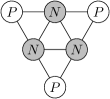
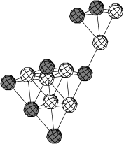
Figure 1. Newton diagram for $n=2$ for $Q(X)=X_{0}^{2}+X_{1}^{2}+X_{2}^{2}-X_{0}X_{1}-X_{1}X_{2}-X_{0}X_{2}$ (on left) and a sample diagram for $n=3$ (on right).

Definition 2.6.

We say two points in the Newton diagram are adjacent if the corresponding monomials $X^{\alpha}$ and $X^{\beta}$ are such that there exist $k$ and $j$ such that $X_{j}X^{\alpha}=X_{k}X^{\beta}$. Between any two points (or any two monomials) we can define the distance $\operatorname{dist}(X^{\alpha},X^{\beta})$ as 1 if the corresponding monomials are adjacent, and if they are not adjacent as the length of the shortest path along adjacent monomials.

The support $K\subset{\mathbb{Z}}^{n}$ of a Newton diagram $D$ is the set of nonzero points. That is, $K=D^{-1}(\{P,N\})$. As $K$ cannot contain any negative coordinates, we will generally consider $K$ a subset of ${\mathbb{N}}_{0}^{n}$ (where ${\mathbb{N}}_{0}=\{0\}\cup{\mathbb{N}}$).

We say that the support $K$ of a Newton diagram $D$ is connected if any two points of $K$ are joined by a path of adjacent points of $K$.

For a set $K\subset{\mathbb{Z}}^{n}$, we let $\widehat{K}\subset{\mathbb{Z}}^{n}$ be the smallest simplex that contains $K$. More precisely, $\widehat{K}\subset{\mathbb{Z}}^{n}$ is the smallest set such that $K\subset\widehat{K}$ and for some $a=(a_{1},\ldots,a_{n})\in{\mathbb{Z}}^{n}$ and some $k\in{\mathbb{N}}$ we have

$$\widehat{K}=\{x\in{\mathbb{Z}}^{n}\mid x_{j}\geq a_{j}\;,\;\left\lvert{x}\right\rvert\leq k\}.$$ (18)

When $K\subset{\mathbb{N}}_{0}^{n}$ then the diameter of $\widehat{K}$ in the distance defined above is easily seen to be $k-\left\lvert{a}\right\rvert$. We define the size of $K$ as the diameter of $\widehat{K}$ plus one.

The adjacency between points in the figures is marked by drawing a line connecting the two circles or spheres. If $P\in{\mathcal{I}}(n)$, then we will show that p-degree of $P$ is equal to the size of $K$ where $K$ is the support of the Newton diagram corresponding to $P$.

Definition 2.7.

Let $D\colon{\mathbb{Z}}^{n}\to\{0,P,N\}$ be a Newton diagram. Let $X^{\alpha}$ be a monomial of degree $d$. Let $E=E(\alpha)$ be the set of points in ${\mathbb{Z}}^{n}$ defined by

$$E:=\{m\in{\mathbb{Z}}^{n}\mid X_{k}X^{\gamma(m)}=X^{\alpha}\text{ for some $k$}\}.$$ (19)

We call $E$ a node if the direct image $D(E)=\{P\}$, $D(E)=\{N\}$, $D(E)=\{0,P\}$, or $D(E)=\{0,N\}$. Do note that we allow negative indices in $E$. For a diagram $D$ let

$$\#(D):=\text{(number of nodes in $D$)}.$$ (20)

See Figure 2 for examples of diagrams with nodes marked. In dimension 2, the nodes are marked with a triangle where each vertex of the triangle touches a point of the node. In dimension 3 we mark the nodes similarly with a simplex.

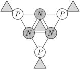
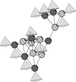
Figure 2. Nodes in Newton diagrams for $n=2$ (on left) and $n=3$ (on right).

The number of nodes $\#(D)$ functions as a lower bound for the number of non-zero coefficients for a polynomial in ${\mathcal{H}}(n,d)$, or rather, as a generalization thereof. Let $p\in{\mathcal{H}}(n,d)$ and let $P$ be the induced homogeneous polynomial with corresponding Newton diagram $D$. If the diagram $D$ has a node at the points of the form $\frac{X_{0}}{X_{j}}X^{\alpha}$, with $\alpha=(\alpha_{0},\alpha^{\prime})$, then it is easy to see that for the polynomial $p$, the coefficient of the monomial $x^{\alpha^{\prime}}$ cannot be zero. The non-negativity of the coefficients of $p$ puts a restriction on the kind of nodes that can occur in each mutually connected collection of nonzero points, but as we are also interested in allowing coefficients of the polynomials $p$ to be negative we will ignore this restriction as much as possible.

In two dimensions it will be sufficient to obtain only the very mild restrictions on the support that are given by the next two lemmas.

Lemma 2.8.

Let $P\in{\mathcal{I}}(n)$. Write $P=S\cdot Q$. Let $D$ be the Newton diagram of $Q$, with support $K$.

1. If $P$ is indecomposable, then $K$ is connected.

2. The size of $K$ is equal to the p-degree of $P$.

Proof.

Let us prove the first item. Suppose that $K$ is disconnected. Then take $K_{1},\ldots,K_{r}$ be the connected components. Define the $Q_{j}$ by taking those monomials of $Q$ that are in $K_{j}$. As if $j\not=k$, then no points in $K_{k}$ is adjacent to any point of $K_{j}$. Therefore $Q_{k}S$ has no monomials in common with $Q_{j}S$. Thus define $P_{j}=Q_{j}S$. We see that $P=P_{1}+\cdots+P_{r}$ and $P$ is decomposable.

Now let us prove the second item. By taking $a=(0,\ldots,0)$ in the definition of $\widehat{K}$ and the size of $K$, it is not hard to see that the size of $K$ is at least the p-degree of $P$. Suppose that $\widehat{K}$ does not contain any points $m\in{\mathbb{Z}}^{n}$ with $m_{1}\leq k$ for some $k$. Then $Q$ is divisible by $X_{1}^{k+1}$. The result follows by iterating through all the variables. ∎

Lemma 2.9.

Let $p\in{\mathcal{H}}(n,d)$, let $P=S\cdot Q$ be the induced homogeneous polynomial and $D$ the Newton diagram of $Q$, with support $K$. Then $K$ is connected, contains $(0,\ldots,0)$ and is of size $d$.

Proof.

First we note that $P$ is indecomposable. Suppose that $P$ were decomposable. That would in fact imply that there would exist two nontrivial polynomials $p_{1}$ and $p_{2}$ with positive coefficients such that $p_{1}+p_{2}=p$, $p_{1}$ and $p_{2}$ are constant on the hyperplane $s=1$, and have no monomials in common. In fact, the constant term in $p-1$ can only be in one of $p_{1}$ or $p_{2}$ and hence one of them is zero on the hyperplane. So suppose that $p_{2}=0$ on $s=1$. As all coefficients of $p_{2}$ are positive, then they are all zero. Hence $p_{2}\equiv 0$. Therefore $P$ is indecomposable.

Thus by Lemma 2.8, $K$ is connected. If we let $q=\frac{p-1}{s-1}$. If $p(0)=1$, then we obtain a contradiction as above, $p-1$ would have all positive coefficients and be zero on $s=1$. Therefore $p(0)\not=1$. Then it is not hard to see that $q$ must contain a nonzero constant. Therefore so does $Q$ and hence $(0,\ldots,0)\in K$.

Once $(0,\ldots,0)\in K$, we see that the size of $K$ cannot be any smaller than $d$. Since for all points $m\in K$ we have $\left\lvert{m}\right\rvert<d$, then $K$ is of size $d$. ∎

In fact, in two dimensions we will be able to prove the estimate on $\#(D)$ without requiring that $(0,0)\in K$. Compare Theorem 3.4 and Proposition 3.1.

Our proof in three dimensions requires stronger restrictions on $K$. We make the following definition.

Definition 2.10.

A set $K\subset{\mathbb{Z}}^{2}$ has left overhang if there exists a point $(a,b)\in K$, $(a,b)\not=(0,0)$ such that $(a,b-1)\notin K$ and $(a-1,y)\notin K$ for all $y\geq b$.

A point $(a,b)\in K$ is right overhang if it is a left overhang after swapping variables. We say simply that $(a,b)$ is an overhang if it is a left or a right overhang.

Let $K\subset{\mathbb{Z}}^{3}$. Define $\pi_{j}\colon{\mathbb{Z}}^{3}\to{\mathbb{Z}}^{2}$, $j=1,2,3$, by $\pi_{1}(m)=(m_{1},m_{2}+m_{3})$, $\pi_{2}(m)=(m_{1}+m_{3},m_{2})$, and $\pi_{3}(m)=(m_{1}+m_{2},m_{3})$. Then we say that $m\in K$ is an overhang if $\pi_{j}(m)$ is an overhang of $\pi_{j}(K)$ for some $j=1,2,3$.

When no overhang exists in $K\subset{\mathbb{Z}}^{n}$ we say that $K$ satisfies the no-overhang condition. We will sometimes say that a Newton diagram $D$ satisfies the no-overhang condition, which means that the support $K$ of $D$ has no overhang. Similarly, when we say that $P\in{\mathcal{I}}(n)$ satisfies the no-overhang condition we mean that the support of the corresponding Newton diagram satisfies the no-overhang condition.

The projection $\pi_{1}$ is equivalent to setting the 2nd and 3rd variable equal to each other in the underlying polynomial. Similarly for $\pi_{2}$ and $\pi_{3}$. The Figure 3 illustrates a diagram with an overhang. The overhang is marked with a circle in the figure. The second view is along one axis signifying the projection of the support by a $\pi_{j}$ for some $j$. The overhang in 2 dimensions is then easy to see.

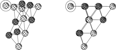
Figure 3. Two views of a diagram violating the no-overhang condition.

Lemma 2.11.

Let $p\in{\mathcal{H}}(n,d)$, $2\leq n\leq 3$, and $P,Q,D,K$ be as in Lemma 2.9. Then $K$ has no overhang.

Proof.

We start with $n=2$. Let $p\in{\mathcal{H}}(2,d)$. Suppose that $(a,b)\in K$ be an overhang. Without loss of generality assume $(a,b)$ is a left overhang. Since $D(a-1,b)=D(a,b-1)=0$, then we have a node and $p$ contains the monomial $x_{1}^{a}x_{2}^{b}$. As $(a,b)\not=(0,0)$, the coefficient of $x_{1}^{a}x_{2}^{b}$ has to be positive. Let $q=\frac{p-1}{s-1}$, the coefficient of $x_{1}^{a}x_{2}^{b}$ must be negative. Because we are multiplying $q$ by $s-1=x_{1}+x_{2}-1$, we note that the coefficient of $x_{1}^{a}x_{2}^{b+1}$ in $q$ must be negative as well, otherwise we would get a negative coefficient of $x_{1}^{a}x_{2}^{b+1}$ in $p$. But that means that the coefficient of $x_{1}^{a}x_{2}^{k}$ in $q$ for all $k\geq b$ must be negative. But $q$ is a polynomial and hence for some $k$, the coefficient is zero. Then we get a negative term in $p$ which is a contradiction. Therefore the lemma holds for $n=2$.

Now let $n=3$. Let $p\in{\mathcal{H}}(3,d)$. Suppose for contradiction that $(a,b,c)\in K$ is an overhang. Without loss of generality suppose that $\pi_{1}(a,b,c)=(a,b+c)$ is an overhang of $\pi_{1}(K)$. For some $t\in(0,1)$, let $\tilde{p}(x_{1},x_{2})=p(x_{1},tx_{2},(1-t)x_{2})$. Define $\tilde{q}=\frac{\tilde{p}-1}{s-1}$. We can pick $t$ such that the coefficient of $x_{1}^{a}x_{2}^{b+c}$ in $\tilde{q}$ is nonzero, which we can certainly do. Let if we homogenize $\tilde{p}$ to create $\tilde{P}$, find $\tilde{Q}$ and the Newton diagram $\tilde{D}$, then if $\tilde{K}$ is the support of $\tilde{D}$, then it is easy to see that $\tilde{K}\subset\pi_{1}(K)$. Furthermore, $(a,b+c)\in\tilde{K}$. If $(a,b+c)$ was an overhang of $\pi_{1}(K)$, then it is an overhang of $\tilde{K}$. The fact that $\tilde{p}\in{\mathcal{H}}(2,d)$ leads to a contradiction. ∎

In the next two sections we will often refer to directions of a support $K$, imagining the $(0,\ldots,0)$ point at the bottom and the points $m$ with $\left\lvert{m}\right\rvert=d-1$ at the top. Note that points at the top correspond to monomials of degree $d-1$ in nonhomogeneous coordinates obtained by setting $X_{0}=1$. Similarly by up (resp. down) we will mean the direction of increasing (resp. decreasing) $\left\lvert{m}\right\rvert$ (that is, degree in nonhomogeneous coordinates). By a side of $K$ we mean a collection of points for which a fixed coordinate is equal to zero. In the two dimensional case we will use left and right without worrying about which is which. By the $k$th level we will mean points $m$ where $\left\lvert{m}\right\rvert=m_{1}+\cdots+m_{n}=k$.

3. Two-dimensional results

Let us start by recalling some ideas of the proof of the $2$-dimensional result by D’Angelo, Kos, and Riehl. We start with a polynomial $p(x,y)$ with non-negative coefficients that satisfies $p=1$ when $s=x+y=1$. We assume that $p$ is of degree $d$ and we wish to estimate from below the number of non-negative coefficients of $p$.

D’Angelo, Kos and Riehl then write $p=(s-1)q+1$ for some polynomial $q$, but instead we will use the induced homogeneous polynomial $P$ and the notation $P=S\cdot Q$ as was introduced in the previous section. We obtain the Newton diagram $D$ of $Q$ and as we discussed in the previous section, the number of nodes of $D$ is a lower estimate for the number of positive coefficients of $p$. The positivity of $p$ puts strong restrictions on the diagram $D$, but for now we only require that the support $K$ of $D$ is connected. We will at first require that $(0,0)\in K$ but we will remove this restriction later.

By manipulating the Newton diagram $D$ without increasing the number of nodes, D’Angelo, Kos and Riehl were able to show that the number of nodes of $D$ must be at least $\frac{d+5}{2}$. Since the node involving the points $(0,0)$, $(0,-1)$, and $(-1,0)$ does not correspond to a positive coefficient of $p$ but all other nodes do, we see that $p$ must have at least $\frac{d+3}{2}$ positive coefficients. Considering that generally many of the coefficients of the polynomial $p$ are ignored when counting nodes, it is truly remarkable that this argument gives the sharp bound for $N(p)$.

Their method is the following: they make small local changes to $D$ such that after every step the number of nodes has not increased and the lowest and left most node has moved to the right or up. After a finite number of steps all nodes must be at the top level and it is then easy to give a lower estimate on the number of nodes.

Instead of following their argument we give a slightly different proof. The reason is that the above argument cannot possibly work in dimensions $3$ and higher. It is not hard to see that if all nodes are at the top level then the estimate on the number of nodes would be at least quadratic in $d$. But since it is easy to give examples where the number of coefficients of $p$ (and thus also the number of nodes of $D$) is at most linear in $d$, it cannot always be possible to push the nodes to the top level without increasing their number. Fortunately the argument that we will give here is also a bit simpler than the original proof.

Instead of manipulating $D$ to remove the lowest nodes, we will repeatedly eliminate the lowest zero, and end up with a Newton diagram that consists entirely of $P$s and $N$s.

Proposition 3.1.

Let $D$ be a Newton diagram with support $K$ in two variables. Suppose that $K$ is of size $d$, is connected, and contains $(0,0)$. Then

$$\#(D)\geq\frac{d+5}{2}.$$ (21)

The proof of Proposition 3.1 will consist of two short lemmas. We will say that a diagram $D^{\prime}$ is an extension of $D$ if the support $K^{\prime}$ of $D^{\prime}$ contains the support $K$ of $D$ and such that $D^{\prime}|_{K}=D|_{K}$.

Lemma 3.2.

Let $D$ and $K$ be as in Proposition 3.1. Let $k<d$ and suppose that $K$ contains all points $a$ with $\left\lvert{a}\right\rvert\leq k-1$. Then there exists an extension $D^{\prime}$ of $D$ that has equal or fewer nodes, and whose support $K^{\prime}$ contains all points $a$ with $\left\lvert{a}\right\rvert\leq k$.

Proof.

We change the $0$-points at level $k$ into alternating $N$- and $P$-points, one connected group of $0$-points of level $k$ at a time. Since there must be at least one $P$- or $N$-point at the $k$-level, there are two cases that we should consider: one is that the group has $N$- or $P$-points on both sides, and the other is that the group extends to one of the boundaries. In the former case no new nodes can be created by changing the points and we are done. In the latter case it is possible to create a node at the boundary, but by choosing the boundary point correctly one boundary node is eliminated as well and we are done. See Figure 4. The circles with the dark borders are the nonzero points that were added in a single step. ∎

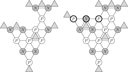
Figure 4. Filling a 2-dimensional diagram.

Using Lemma 3.2 repeatedly we obtain a diagram with support $K=\{(a,b)\in{\mathbb{N}}_{0}^{2}\mid a+b<d\}$. Proposition 3.1 now follows from the following Lemma:

Lemma 3.3.

Let $D$ be a Newton diagram in two variables with support $K$ of size $d$ and suppose that $K$ is maximal: it contains all $(a,b)\in{\mathbb{N}}_{0}^{2}$ with $a+b<d$. Then $D$ has at least $\frac{d+5}{2}$ nodes.

Proof.

Let us consider a horizontal row $\{(a,b)\in{\mathbb{N}}_{0}^{2}\mid a+b=k\}$ at level $k<d-1$. Suppose that, starting with $(k,0)$ and ending with $(0,k)$, the sign changes $m$ times from $P$ to $N$ or vice-versa. Also suppose that there are $n$ sign changes on the next higher row $\{(a,b)\mid a+b=k+1\}$. Then there are at least $\frac{\left\lvert{m-n}\right\rvert}{2}$ nodes involving points only on these two rows.

Now suppose that there are $l$ sign changes on the highest row $\{(a,b)\mid a+b=d-1\}$. Then there are exactly $d-l+1$ nodes on this highest row. Since there are zero sign changes on the lowest row $\{(0,0)\}$, it follows from the observation in the previous paragraph that there must be at least $\frac{l}{2}$ nodes involving some point $(a,b)$ with $1<a+b<d-1$, as well as the one node involving the points $(0,0),(-1,0)$ and $(0,-1)$. Adding the three numbers gives a total of at least $d-\frac{l}{2}+2$ nodes. The minimum number of nodes can therefore only be achieved when $l=d-1$, the maximum number of sign changes on the row $\{(a,b)\mid a+b=d-1\}$. Inserting $l=d-1$ shows that there are at least $\frac{d+5}{2}$ nodes. ∎

We end this section with the proof of Theorem 2.4. We will prove the following stronger result about Newton diagrams that at once implies Theorem 2.4.

Theorem 3.4.

Let $D$ be a Newton diagram with connected support $K$ of size $d$ in two variables. Then

$$\#(D)\geq\frac{d+5}{2}.$$ (22)

Proof.

Without loss of generality we may assume that the support $K$ contains points on both sides, that is point $(a,0)$ and a point $(0,b)$. By connectedness $K$ must contain a connected path from the left side to the right. By the proof of Lemma 3.2 we can change all the $0$-points of $D$ above this connected path into $P$- and $N$-points without increasing the number of nodes. By switching the roles of $X_{0}$ and $X_{1}$ we then obtain a new Newton diagram with the same number of nodes whose support is connected, of size $d$ and contains $(0,0)$, which by Proposition 3.1 completes the proof. ∎

4. Preparing for three dimensions

The main idea that we use for estimating the number of nodes of a $3$-dimensional Newton diagram $D$ is to ignore the nodes that might occur in the interior of the diagram and to only count the number of nodes that occur on each of the faces of the support $K$. For each of these faces we can then use two dimensional estimates. Of course, by counting the number of nodes on each face separately and then adding the estimates we are in danger of counting some nodes more than once, namely nodes involving points that lie on more than one face. We therefore adjust the node count.

Definition 4.1.

Let $D$ be a $2$-dimensional Newton diagram. A node that involves no zeroes is called an interior node, a node with exactly one zero is called an edge node, and a node with two zeroes is called a vertex node. When both zeroes of a vertex node lie at the bottom of the node, the node is called a bottom node.

The weighted surface count of $D$ is the number of interior nodes, plus half the number of edge and vertex nodes, but ignoring the number of corner nodes:

$$SC(D):=\text{(\# of interior nodes)}+\frac{1}{2}\times\Bigl{(}\text{(\# of edge nodes)}+{}\\ \text{(\# of vertex nodes)}-\text{(\# of bottom nodes)}\Bigr{)}.$$ (23)

Essentially the same proof as that of Lemma 3.3 gives us then the following, perhaps somewhat surprising result. While edge nodes have weight only $\nicefrac{{1}}{{2}}$, we still get the same estimate.

Lemma 4.2.

Let $D$ be a Newton diagram in two variables with support $K$ of size $d$ and suppose that its support $K$ is maximal, that is, contains all $(a,b)$ with $a+b<d$. Then

$$SC(D)\geq\frac{d+1}{2}.$$ (24)

Proof.

As we said, the proof is similar to proof of Lemma 3.3. Again, we consider two adjacent levels in the diagram. If the higher level has $n$ sign changes and the lower level has $m$ sign changes then there must be at least $\frac{\left\lvert{m-n}\right\rvert}{2}$ nodes involving points only on these two levels. This weighted count now includes half nodes at the edges.

What is left is to count the edge nodes that only involve the top level. There are always 2 vertex nodes, plus if there $m$ sign changes at the top level, then there are $d-m-1$ edge nodes. An induction argument completes the proof. ∎

The result is surprising because even though the nodes on the edges and at the vertices have weight only half, we still obtain the same estimate as in Lemma 3.3, except for the obvious two times $\nicefrac{{1}}{{2}}$ that we lose for the two vertex nodes on the top level and the $1$ that we lose for the bottom node. Thus Lemma 3.3 follows immediately from Lemma 4.2. Do note that we now allow more half nodes at the edge. Therefore for a diagram with $d$ edge nodes and 3 vertex nodes we again obtain $SC(D)=\frac{d+1}{2}$.

The result in Lemma 4.2 is necessarily also sharp but we even have this stronger sharpness result that will be useful later:

Lemma 4.3.

Let $D$ be a maximal Newton diagram with support of size $d$. Then we can find a Newton diagram $\tilde{D}$ with support of size $d$ that is maximal, agrees with $D$ for all $(a,b)$ with $a+b=d-1$ and such that $SC(D)$ is exactly equal to $\frac{d+1}{2}$.

Proof.

Construct the example level by level, starting with the top level, which is already determined by $D$. Each next lower level is obtained by removing the leftmost entry of the previous level, and then changing all the signs (so $P$ becomes $N$ and vice verse). Using this construction there cannot be any interior nodes, and the number of edge nodes on the sides is equal to the number of sign changes on the top level. The number of edge nodes on the top level is equal to $d-1$ minus the number of sign changes. Adding these two numbers plus the two vertex nodes on the top level gives $d+1$ nodes that each have weight $\nicefrac{{1}}{{2}}$. ∎

In the three dimensional proof we will perform several different operations on $3$-dimensional Newton diagrams that change the shape of one or more faces. We end the section with three $2$-dimensional lemmas that will be needed to estimate how the number of nodes on the faces change with these operations.

Lemma 4.4.

Let $D$ be a two-dimensional Newton diagram, and suppose that its support $K$ contains all points $(a,b)$ with $a+b<k$ and at least one point $(a,b)$ with $a+b=k$. Then there exist a Newton diagram $\tilde{D}$ that is an extension of $D$ (i.e. the $P$- and $N$-nodes remain unchanged) and the support $\tilde{K}$ of $\tilde{D}$ contains all points $(a,b)$ with $a+b=k$ and satisfies

$$SC(\tilde{D})\leq SC(D).$$ (25)

Finally the set $\tilde{K}\setminus K$ only contains points $(a,b)$ with $a+b=k$.

Proof.

The proof is similar to that of Lemma 3.2 except that we need to be slightly more careful because different kinds of nodes receive different weights. This time we change only one $0$-point at the time, starting with a $0$-point that lies to the left or to the right of a $P$- or $N$-point. By assigning to this point a $P$ or an $N$, there are a number of nodes of $D$ that have weight $\nicefrac{{1}}{{2}}$ but that by the change either receive weight $1$ or are no longer a node, depending on the sign we assign to the $0$-point. The situation for these nodes is completely symmetric: if assigning a $P$ adds $c$ to the weighted surface count then assigning an $N$ subtracts $c$ to the weighted surface count, where $c$ is a multiple of $\nicefrac{{1}}{{2}}$. There is also at most one bottom node of $D$ that has no weight, but that can turn into an edge node of $\tilde{D}$, adding $\nicefrac{{1}}{{2}}$ a node to the weighted surface count depending on the choice of sign. Now it is easy to see what can be done:

If $c=0$ then we can choose the sign such that no bottom node is changed into an edge node. If $c\neq 0$ then we choose the sign such that the weighted surface count is decreased by at least one half from the old $\nicefrac{{1}}{{2}}$-nodes, and since the gain from the potential bottom node that changes into an edge node is at most $\nicefrac{{1}}{{2}}$, the weighted surface count cannot increase. ∎

Lemma 4.5.

Let $D$ be a Newton diagram with support $K$. Suppose that for some $k$, $(a,b)\in K$ whenever $a+b<k$ and $(0,b),(1,b-1)\notin K$ when $b\geq k$. Then define $K^{\prime}\subset{\mathbb{Z}}^{2}$ by

$$K^{\prime}=\{(a,b)\in{\mathbb{Z}}^{2}\mid(a,b+1)\in K\}.$$ (26)

Then there exists a Newton diagram $D^{\prime}$ with support $K^{\prime}$ such that

$$SC(D^{\prime})\leq SC(D)-\frac{1}{2}.$$ (27)

Proof.

We can define $D^{\prime}$ naturally by assigning $D^{\prime}(a,b)=D(a,b+1)$. The estimate follows immediately. ∎

Lemma 4.6.

Let $D$ be a Newton diagram with support $K$ such that for some $k$, $(a,b)\notin K$ whenever $a+b<k$. Suppose that $K$ contains at least one point $(a,b)$ with $a+b=k$. Define

$$K^{\prime}=K\cup\{(a,b)\in{\mathbb{N}}_{0}^{2}\mid a+b<k\}.$$ (28)

Then there is a Newton diagram $D^{\prime}$ with support $K^{\prime}$ such that $SC(D^{\prime})\leq\frac{k}{2}+SC(D)$.

Proof.

By Lemma 4.3 we know that given any choices for the level $\{(a,b)\mid a+b=k-1\}$, there exist a Newton diagram $E$ of degree $k-1$ with the chosen top level and maximal $K$ such that the $SC(E)=\frac{k+1}{2}$. We can choose the top level of $E$ such that by merging $E$ with $D$ no new interior nodes are created, and such that at least one top level edge node of $E$ is canceled by a point of $D$ at level $k$. If $D^{\prime}$ is the Newton diagram obtained by merging $E$ with $D$ then it follows that

$$SC(D^{\prime})\leq\frac{k+1}{2}+SC(D)-\frac{1}{2}.$$ (29)

∎

5. Three-dimensional results

Before we start proving our main result, where we use two-dimensional estimates to do a weighted count of the number of nodes that must occur on each of the faces of a Newton diagram, we should first carefully define what we mean by a face.

Definition 5.1.

A face point of a Newton diagram $D$ with support $K$ is a point of $K$ that is adjacent to a $0$-point. A vertical face of $K$ is a maximal connected family of face points $a=(a_{1},\ldots,a_{n})$ that lie in a plane $\{a_{j}=C\}$. A horizontal face is a maximal connected family of face points that lie in a plane $\{\left\lvert{a}\right\rvert=C\}$.

We can think of a simplex centered at each point of $K$. Then the union of the simplices form a polyhedron. Then faces of the polyhedron correspond to the faces of $K$ as defined above. See Figure 5 where a vertical face is shaded.

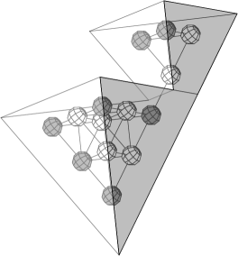
Figure 5. Face in a Newton diagram.

For each face $F$ of $K$ we define $\#(F)$ as the minimal number of nodes that must occur for any possible configuration $F\rightarrow\{0,P,N\}$, but counting only nodes that involve only points of $F$ and points that do not lie in $K$. In other words, if it is possible for a node in $F$ to be cancelled by $N$- or $P$-points outside the face $F$, we assume that they are cancelled.

As before, we write $SC(F)$ for the number of nodes of $F$ (as above) but weighting edge nodes as $\nicefrac{{1}}{{2}}$, weighting vertex nodes in vertical faces as $\nicefrac{{1}}{{2}}$ except for bottom nodes, and not counting bottom nodes in all faces and vertex nodes in horizontal faces. We get the following inequality:

$$SC(D):=\cup_{F}SC(F)\leq\#(D).$$ (30)

Where $F$ ranges over all the faces of $K$. Since bottom nodes are not counted for $SC(D)$ we obtain that

$$SC(D)\leq\#(D)-\text{(\# of bottom nodes)}.$$ (31)

We prove the following result:

Theorem 5.2.

Let $D$ be a 3-dimensional Newton diagram with support $K$ of size $d$, and assume that $K$ has no overhang. Then $D$ has at least $2d+2$ nodes.

Proof.

We will actually prove a stronger statement. Instead of estimating the number of nodes of $D$, we estimate for each face of $K$ the number of nodes that must at least occur on that face of $K$, and add those numbers. Of course by doing so a node that occurs on more than one face will be counted more than once.

A node that occurs at an edge (which means two of the involved points must be $0$) will be counted twice, and a node that occurs at a vertex (which means three of the involved points are $0$) is counted three times. In order to get the right count we will give weight $\nicefrac{{1}}{{2}}$ to the edge nodes for each face. Vertex nodes are only counted (with weight $\nicefrac{{1}}{{2}}$) on vertical faces, and only when they are not bottom nodes (otherwise they have weight zero).

Definition 5.3.

Let $K$ be the support of a $3$ dimensional Newton diagram $D$, and let $K_{1},\ldots,K_{n}$ be the two dimensional faces of $K$. For a vertical face $K_{j}$ we define

$$SC(K_{j})=\min_{D_{j}}SC(D_{j}),$$ (32)

where the minimum is taken over all $2$-dimensional Newton diagrams $D_{j}$ with support $K_{j}$. For a horizontal face we use the same definition except that none of the vertex nodes are counted at all (all have weight zero), so then

$$SC(D_{j})=\text{(\# of interior nodes)}+\frac{1}{2}\times\text{(\# of edge nodes)}.$$ (33)

Finally we define

$$SC(K)=\sum SC(K_{j}).$$ (34)

Of course the number we obtain is a lower estimate and does not have to be equal to the actual number of nodes of $D$ for several reasons. First, interior nodes are not accounted for. Second, the $2$-dimensional Newton diagrams $D_{j}$ do not have to correspond to the diagrams on the faces of $D$. In fact, we don’t require that the Newton diagrams $D_{j}$ “match” at all, so there may not be any Newton diagram $D$ that has optimal $D_{j}$ as faces. Finally, bottom nodes all have weight 0, so for each bottom node we count one node too few. Nevertheless we will be able show that the sum is at least $2d+1$, and since there is at least one bottom node (the node involving the point $(0,0,0)$), this will conclude the proof of the theorem.

Before giving the specifics, we note that we can assume that the p-degree of a polynomial corresponding to $D$ is $d$. That is, we could translate $K$ to assume that for each $j=1,2,3$, there is a point $m\in K$ such that $m_{j}=0$, but still assume that $K\subset{\mathbb{N}}_{0}^{3}$. Now by requiring that $K$ has no overhang, it is not hard to see that $K$ must contain the point $(0,0,0)$.

For the purpose of contradiction we assume that there exists a $K$ with $SC(K)<2d+1$. Let the $d$ be the smallest size for which such $K$ exists. Further assume that for this $d$ the number of points of $K$, $\left\lvert{K}\right\rvert$ is maximal, i.e. the number of $P$s and $N$s of $D$ are maximal.

Now look at the largest $k$ so that $(a,b,c)\in K$ whenever $a+b+c<k$. Either $k=d$ or $k<d$.

If $k=d$ then we can estimate the number of surface nodes of $K$ by applying the estimates obtained in § 3 to each of the sides of the tetrahedron $K$. For each of the three vertical faces we obtain the estimate $\frac{d+1}{2}$ by Lemma 4.2 and for the horizontal face only $\frac{d-1}{2}$ since the three vertex nodes have weight zero. In total we obtain that $SC(K)\geq 2d+1$, which contradicts our assumption.

Therefore we may assume that $k<d$. Now we look at the plane $S_{k}=\{(a,b,c)\in{\mathbb{N}}_{0}^{3}\mid a+b+c=k\}$. Then there are two possibilities. Either $K\cap S_{k}$ contains at least one element on each of the edges $\{(0,b,c)\}$, $\{(a,0,c)\}$ and $\{(a,b,0)\}$, or $K\cap S_{k}$ does not contain an element on one of these edges. Let us deal with the latter case first.

One of the edges is empty: Slice off a face.

In this case we may without loss of generality assume that $K\cap S_{k}$ does not contain elements of the form $(0,b,c)$. Then it follows from the no overhang condition that $K$ does not contain any elements of the form $(0,b,c)$ with $b+c\geq k$. Therefore if we remove from $K$ all elements of the form $(0,b,c)$ and we subtract $1$ from the first coordinate of all remaining elements of $K$, we obtain a new subset $K^{\prime}\subset{\mathbb{N}}_{0}^{3}$ that satisfies the hypotheses of the theorem, except that it now has size $d-1$. See Figure 6. By the assumption on the minimality of $d$ we have that the number of surface nodes of $K^{\prime}$ must be at least $2d-1$. The contradiction therefore follows if we show that $SC(K^{\prime})$ is at least $2$ smaller than $SC(K)$.

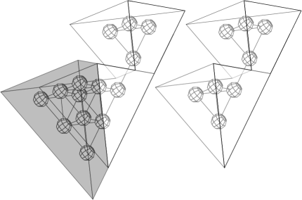
Figure 6. Slicing off a face.

Fortunately almost all the faces of $K^{\prime}$ are equal to those of $K$. There are two side faces that lose one line, namely the faces in the $(b=0)$- and $(c=0)$-planes. Both of these faces lose $\nicefrac{{1}}{{2}}$ a surface node by Lemma 4.5. The horizontal face in the $S_{k-1}$-plane also loses one line but it may or may not lose half a node. If the intersection $K\cap S_{k}\cap\{(1,b,c)\}$ is empty then it is clear that the horizontal face does lose half a node. To see this, we refer back to the proof of Lemma 4.2. If the intersection is empty, we have removed a full line of points from the face, thus removing at least half a node. However, if this intersection is non-empty then the horizontal face may not lose surface nodes (keep in mind that vertex nodes have weight zero for the horizontal faces).

One direction remains to be considered. If $K\cap S_{k}\cap\{(1,b,c)\}$ is empty then the face $K\cap\{(0,b,c)\}$ is replaced by the face $K^{\prime}\cap\{(0,b,c)\}$, which is just a triangle with side length one smaller. Therefore the weighted surface count for this smaller triangle is one-half smaller and the estimate is complete. When $K\cap S_{k}\cap\{(1,b,c)\}$ is not empty the situation is slightly more complicated. Again we lose the surface nodes on the face $K\cap\{(0,b,c)\}$, but we gain nodes when the faces of $K$ in the plane $\{(1,b,c)\}$ are glued to the triangle $\{(1,b,c)\mid b+c<k-1\}$. In this case it follows from Lemma 4.6 that we lose at least $1$ node which completes the estimate.

None of the edges is empty: Fill $S_{k}$.

The only case that is left to deal with is when $K\cap S_{k}$ contains at least one element on each of the edges $\{(0,b,c)\}$, $\{(a,0,c)\}$ and $\{(a,b,0)\}$. The idea now is to take enlarge $K$ by defining $K^{\prime}=K\cup S_{k}$. See Figure 7. By our assumption on $k$ we have that $\left\lvert{K^{\prime}}\right\rvert$ is strictly larger than $\left\lvert{K}\right\rvert$, and $K^{\prime}$ satisfies the no-overhang condition as well. If we can show that the number of surface nodes of $K^{\prime}$ is not larger than that of $K$, then we get a contradiction with our assumption that $\left\lvert{K}\right\rvert$ is maximal.

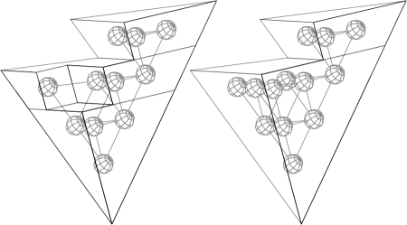
Figure 7. Filling a 3-dimensional Newton diagram.

We apply Lemma 4.4 to see that the number of surface nodes on each of the side faces $\{a=0\},\{b=0\}$, and $\{c=0\}$ does not increase when we extend $K$ to $K^{\prime}$. All the other vertical faces can only become smaller when we replace $K$ by $K^{\prime}$, so the number of surface nodes on those faces only become smaller.

The only faces that are left are the horizontal faces on the levels $k-1$ and $k$. Let us say that we start with some optimal $2$-dimensional Newton diagrams $D_{j}$ with supports $K_{j}$ corresponding to the horizontal faces at levels $k-1$ and $k$ for set $K$. We create a configuration for the horizontal face of $K^{\prime}$ at level $k$ as follows.

We keep the same Newton diagrams for the faces at level $k$ that we already had. We replace every $0$ at level $k$ of $K$ and coordinate $(a,b,c)$, where $a\neq 0$, by the sign of the point $(a-1,b,c)$ of the Newton diagram $D_{j}$ containing that point, although it is possible that we need to reverse all the signs for a face $D_{j}$, as we shall see below. After we have done this procedure, we will see that we can assign signs to the remaining $0$-points of the form $(0,b,c)$ with $b+c=k$ in a way that does not increase the number of nodes.

By sliding the faces at level $k$ upwards in this way there can only be fewer internal nodes, as the faces can become smaller but not larger. There are vertex (or edge) nodes that remain vertex (or edge) nodes so we do not need to worry about those. However, when ‘gluing’ these configurations to the configurations of the old faces at level $k$ it is also possible for edge and vertex nodes to become internal nodes, which have weight one. This is possible in two different ways.

The first way is for an vertex node of an old $k$-level face to become an internal node. Since the horizontal vertex had weight zero, this gives us one extra node, but as we remarked earlier, we lose twice half a node on vertical faces when such a vertex becomes internal, so we do not need to worry about this case.

The other way is for an edge node of an old $k$-level face to become an internal node. We can deal with this case by flipping the signs of old level $k$ configurations. By doing this we get that at most half of the edge nodes of old configurations that actually become internal nodes, and the other edge nodes disappear, which solves this case as well.

That leaves us with the remaining $0$-points on the edge $\{(0,b,c)\mid b+c=k\}$. As we only have to worry about the horizontal faces (as the weighted count for the vertical faces is already taken care of) and vertex-nodes in horizontal faces have weight zero, it is easy to assign $P$ or $N$ to each point one by one, starting with points adjacent to non-$0$ points in the edge (which we assumed exist), in such a way that no interior nodes are created and the number of edge nodes remains the same. This completes the proof. ∎

6. Sharp polynomials in three dimensions

In the previous section we have obtained some information of what a Newton diagram with minimal number of nodes looks like. While it is not hard to construct a polynomial $Q$ corresponding to a given Newton diagram, in general we will get many more nonzero terms in the corresponding $P\in{\mathcal{I}}(3)$ than there are nodes in the diagram.

We will say an indecomposable polynomial $P\in{\mathcal{I}}(n,d)$ is sharp if $N(P)$ is minimal among all indecomposable polynomials ${\mathcal{I}}(n,d)$. We make a similar definition for ${\mathcal{H}}(n,d)$; $p\in{\mathcal{H}}(n,d)$ is sharp if $N(p)$ is minimal in ${\mathcal{H}}(n,d)$. We will concentrate on ${\mathcal{H}}(n,d)$ in this section since we have proved sharp bounds only for ${\mathcal{H}}(3,d)$ and not for ${\mathcal{I}}(3,d)$. Also using the nonhomogeneous notation will make the computations and the exposition simpler. Of course, if it turns out that indecomposable polynomials in ${\mathcal{I}}(3,d)$ posses the same degree bounds as ${\mathcal{H}}(3,d)$, then the sharp polynomials we describe in this section will also be sharp in ${\mathcal{I}}(3,d)$.

It is an easier problem to list all possible Newton diagrams with the sharp number of nodes, but it is harder to decide which diagrams correspond to actual sharp polynomials in ${\mathcal{I}}(n,d)$ or ${\mathcal{H}}(n,d)$. For $n=2$ the classification of sharp polynomials is not trivial even in ${\mathcal{H}}(2,d)$, see [DL:complex, LL]. We will see that classification in dimension 2 is related to classifying the sharp polynomials in dimension 3.

It is not hard to construct certain sharp polynomials $p\in{\mathcal{H}}(3,d)$. That is, $p$ achieves equality in the bound

$$\deg(p)\leq\frac{N(p)-1}{2}.$$ (35)

Start with

$$p_{1}(x):=s(x)=x_{1}+x_{2}+x_{3}.$$ (36)

Now construct

$$p_{d}(x):=p_{d-1}(x)-x_{3}^{d-1}+x_{3}^{d-1}(s(x)-1).$$ (37)

It is not hard to see that $p_{d}\in{\mathcal{H}}(3,d)$ and that $N(p_{d})=N(p_{d-1})+2$, and therefore $N(p_{d})=2d+1$. Thus, $p_{d}$ are sharp. These polynomials are known (see for example [DLP]) as generalized Whitney polynomials. At each step, instead of $x_{3}^{d-1}$ we can also pick an arbitrary monomial of $p_{d-1}$ of degree $d-1$. We then obtain all the other generalized Whitney polynomials.

The Newton diagram for the Whitney polynomials is easy to see. In the nonhomogeneous setup, where we just take the Newton diagram of $q=\frac{p-1}{s-1}$, the diagram is simply a connected path of $d$ $P$s going from $(0,0,0)$ to $(a,b,c)$ where $a+b+c={d-1}$. In the homogeneous setup, the signs are not all $P$, but instead alternate between $P$ and $N$.

It is natural to ask what all the sharp polynomials look like. In particular, one might wonder if there are there any examples that are not generalized Whitney polynomials. The following construction was given in [DLP]. Start with

$$x_{1}^{3}+3x_{1}x_{2}+x_{2}^{3},$$ (38)

which is sharp and is in ${\mathcal{H}}(2,3)$. Now replace $x_{2}$ with $x_{2}+x_{3}$ to obtain

$$\begin{split}p(x)&:=x_{1}^{3}+3x_{1}(x_{2}+x_{3})+(x_{2}+x_{3})^{3}\\ &\phantom{:}=x_{1}^{3}+3x_{1}x_{2}+3x_{1}x_{3}+x_{2}^{3}+3x_{2}^{2}x_{3}+3x_{2}x_{3}^{2}+x_{3}^{3}.\end{split}$$ (39)

The $p$ obtained is in ${\mathcal{H}}(3,3)$, and furthermore it has $2d+1=7$ terms and hence is sharp. The obtained Newton diagram has maximal support, that is, the support $K$ of the diagram contains all points $m$ such that $\left\lvert{m}\right\rvert<d$. For degrees up to 7 we can prove the following proposition.

Proposition 6.1.

Suppose that $p\in{\mathcal{H}}(3,d)$ is sharp and that the induced Newton diagram has maximal support $K$ (that is, $K$ contains all points $m\in{\mathbb{N}}_{0}^{3}$ with $\left\lvert{m}\right\rvert<d$). Also assume that $d\leq 7$. Then up to permutation of variables, $p$ is equal to either $s$ or (39).

We conjecture that this proposition holds for all degrees. Before we prove the proposition, we will need the following lemma. See [DLP] and [DKR] for proof and more discussion of these results.

Lemma 6.2.

Let $p\in{\mathcal{H}}(n,d)$.

1. If $p$ is homogeneous of degree $d$, then $p=s^{d}$.

2. Write

   $$p(x)=\sum_{\left\lvert{\alpha}\right\rvert=d}c_{\alpha}x^{\alpha}+\sum_{\left\lvert{\alpha}\right\rvert<d}c_{\alpha}x^{\alpha},$$ (40)

   then we have

   $$p(x)=s^{d}+\sum_{\left\lvert{\alpha}\right\rvert<d}c_{\alpha}x^{\alpha}\left(1-s^{d-\left\lvert{\alpha}\right\rvert}\right).$$ (41)

Proof of Proposition 6.1.

First homogenize $p$, then change variables to obtain a polynomial $P$ in ${\mathcal{I}}(3)$. By setting each variable to zero in turn, we obtain four 2-dimensional diagrams with maximal support for polynomials in ${\mathcal{I}}(2)$.

Let $D_{1},\ldots,D_{4}$ be the 2-dimensional diagrams obtained above. We notice that $N(P)$ is bounded below by the number $SC(D_{1})+SC(D_{2})+SC(D_{3})+SC(D_{4})+1$. Now each $SC(D_{i})$ is bounded below by $\frac{d+1}{2}$ using Lemma 4.2.

The following statements are easy to verify for sharp polynomials. If $p\in{\mathcal{H}}(3,d)$ is sharp and the corresponding Newton diagram has maximal support, then:

1. There exists no term in $p$ of degree strictly less than $d$ depending on all 3 variables.

2. For each $i=1,2,3$, there is precisely one pure term $x_{i}^{d}$.

3. For each $i=1,2,3$, the number of non-pure terms not depending on $x_{i}$ is bounded below by $\frac{d-1}{2}$ if we weight terms of degree $d$ as $\nicefrac{{1}}{{2}}$ a term and terms of degree less than $d$ have weight 1.

4. The number of non-pure degree-$d$ terms is bounded below by $\frac{d-1}{2}$ if we weight terms that depend on only 2 variables for $\nicefrac{{1}}{{2}}$ a term and the terms that depend on all 3 variables for 1 term.

The reason for weighting some terms for $\nicefrac{{1}}{{2}}$ is, of course, because we count them twice, once when counting the degree-$d$ terms and once when counting terms not depending on a certain variable. The item (i) follows because the polynomial is sharp, and $\sum_{j=1}^{4}SC(D_{j})$ is already the sharp number. Item (ii) was noticed by [DKR]. It follows because a diagram for a polynomial in ${\mathcal{H}}(2,d)$ that has maximal support can only contain one node for a pure term degree $d$. If there were any other node for a pure term, it would force a negative pure term in $p$.

Now we use Lemma 6.2. We start with $s^{d}=(x_{1}+x_{2}+x_{3})^{d}$. We are allowed to subtract from $s^{d}$ polynomials of the form

$$c_{\alpha}x^{\alpha}\left(1-s^{d-\left\lvert{\alpha}\right\rvert}\right).$$ (42)

where $x^{\alpha}$ does not depend on a single variable and is of degree $d-1$ or less. We are only allowed to subtract polynomials of the form (42) such that we do not violate the bounds given above. In particular, we are only allowed to subtract (42) for terms $x^{\alpha}$ where $x^{\alpha}$ does not depend on all variables; that is, it is independent of at least one variable. For example, for $d=7$ we are allowed to do up to 3 such subtractions for each missing variable (so altogether up to 9 subtractions). We must ensure that the subtractions also remove enough terms of degree $d$.

It is not hard but it is tedious to check all the possibilities for low degrees. We have verified the claim up to $d\leq 7$. We leave the details to the reader. ∎

Proposition 6.1 together with the geometric insight from the proof of the main result seem to suggest to the authors that the following construction generates all sharp $p\in{\mathcal{H}}(3,d)$. Start with $p$ being either $s$ or the polynomial (39), possibly with permuted variables. Then construct others inductively. Pick a sharp $p\in{\mathcal{H}}(3,d)$, pick a monomial $m$ in $p$ of degree $d$. Let $g$ be either $s$ or the polynomial (39) (possibly with permuted variables). Construct $\tilde{p}$ as

$$\tilde{p}:=p-m+mg.$$ (43)

It is easy to see that $\tilde{p}\in{\mathcal{H}}(3,d+k)$, where $k=1$ if $g=s$ or $k=3$ if $g$ was (39). Furthermore, $\deg{\tilde{p}}=\frac{N-1}{2}$, so $\tilde{p}$ is sharp.

7. Higher dimensions

It would have been welcome if the methods that we have developed so far were applicable in higher dimensions. Unfortunately the combinatorics in dimensions $4$ and higher is considerably different. The proof of the main estimate cannot possibly work for the following reason. We prove the main sharp estimate by noting that we can in some sense fill the whole diagram. Such a technique must always fail in higher dimensions. We make the following observation.

For $n\geq 4$, a Newton diagram $D$ with support $K$ of size $d\geq 2$ such that $K$ contains all $m\in{\mathbb{N}}_{0}^{n}$ with $\left\lvert{m}\right\rvert<k$ has too many nodes.

Here too many means more than $d(n-1)+2$ nodes. There exist indecomposable polynomials in ${\mathcal{I}}(n,d)$ with precisely $d(n-1)+2$ terms. These are induced by the generalized Whitney polynomials as described in the previous section or in [DLP]. These polynomials are in ${\mathcal{H}}(n,d)$ and have $d(n-1)+1$ positive terms. Therefore, the sharp estimate for $n\geq 2$, cannot be obtained by looking at a completely filled Newton diagram.

Next we verify this observation. We will only count nodes that appear on two-dimensional faces of the filled-in diagram. It also suffices to only consider $n=4$. For $n=4$, the support has 10 two-dimensional faces. Let $D$ be the completely filled diagram in 4 dimensions. Let us not count the vertex nodes as there are exactly 5 of those. Let us write $D_{f}$ for a diagram of a face. Each edge node of $D_{f}$ contributes $\nicefrac{{1}}{{3}}$ to the total weighted count of $\#(D)$, as we count each edge 3 times. Each face node contributes $1$ to $\#(D)$. If we look at the proof of Lemma 4.2, we notice that

$$\frac{1}{3}\times\text{(\# of edge nodes)}+\text{(\# of face nodes)}\geq\frac{d-1}{3}.$$ (44)

The way to minimize this number is to only have edge nodes. We then must have $d-1$ edge nodes. Hence for $d>1$ we have

$$\#(D)\geq 10\left(\frac{d-1}{3}\right)+5>3d+2.$$ (45)

As noted above, the generalized Whitney polynomials constructed in [DLP] and the previous section for $n=4$ give diagrams with exactly $3d+2$ nodes.

In particular, no example such as (39) exists when $n>3$. In [DLP] it was proved that for $n$ sufficiently large compared to the degree $d$, all sharp polynomials in ${\mathcal{H}}(n,d)$ are generalized Whitney polynomials. With the geometric insight and the techniques developed in this paper, the authors conjecture that all sharp polynomials in ${\mathcal{I}}(n)$, $n\geq 4$ are Whitney.

While we are not able to prove the sharp bound for larger dimensions, we can use the $n=2$ results to prove a degree bound (alas not sharp) for indecomposable polynomials in ${\mathcal{I}}(n)$ for all $n\geq 3$ without the positivity requirement. We will follow the pullback procedure from [DLP] to prove the following bound.

Theorem 7.1.

Let $P\in{\mathcal{I}}(n)$, $n\geq 3$ be indecomposable and suppose that $P$ contains one pure monomial. Then

$$\operatorname{p-degree}(P)\leq\frac{2n(2N(P)-5)}{3n^{2}-3n-2}\leq\frac{4}{3}~{}\frac{2N(P)-5}{2n-3}.$$ (46)

The bound is slightly different from [DLP] and (8) only because in the projectivized version we count one extra term. The following proof and computation is essentially the same as in [DLP] but is adapted to our setting and slightly simplified.

Proof.

Let $P\in{\mathcal{I}}(n)$, $n\geq 3$ be indecomposable and suppose that $P$ contains the monomial $X_{n}^{d}$. That is we can write

$$P(X)=(X_{0}+X_{1}+X_{2}+\cdots+X_{n})Q(X).$$ (47)

Let $D=2n-3$. Now take the sharp degree $D$ polynomial mapping $\phi$ from [DKR], which has the homogenized form

$$(u,v,t)\mapsto(u^{D},v^{D},c_{1}u^{D-2}vt,c_{2}u^{D-4}v^{2}t^{2},\ldots,t^{D}).$$ (48)

The precise values of $c_{j}$ are not important for us. This map has exactly $n+1$ components and furthermore

$$u^{D}+v^{D}+c_{1}u^{D-2}vt+c_{2}u^{D-4}v^{2}t^{2}+\cdots-t^{D}=(u+v-t)q(u,v,t).$$ (49)

If we swap $t$ for $-t$ we obtain a map $\tilde{\phi}$

$$(u,v,t)\mapsto(u^{D},v^{D},-c_{1}u^{D-2}vt,c_{2}u^{D-4}v^{2}t^{2},\ldots,t^{D})$$ (50)

that is

$$u^{D}+v^{D}-c_{1}u^{D-2}vt+c_{2}u^{D-4}v^{2}t^{2}-\cdots+(-1)^{D+1}t^{D}=(u+v+t)\tilde{q}(u,v,t).$$ (51)

We modify $P$ to create $\tilde{P}$ by replacing $X_{2}$ with $-X_{2}$, $X_{4}$ with $-X_{4}$ and so on

$$\tilde{P}(X):=(X_{0}+X_{1}-X_{2}+\cdots+(-1)^{D+1}X_{n})\tilde{Q}(X).$$ (52)

The signature of $(X_{0}+X_{1}-X_{2}+\cdots+(-1)^{D+1}X_{n})$ is exactly the same as the signature of $\tilde{\phi}$. Furthermore $N(\tilde{P})=N(P)$. We can now compose $\tilde{P}\circ\tilde{\phi}$ and note that

$$(\tilde{P}\circ\tilde{\phi})(u,v,t)=(u+v+t)q_{1}(u,v,t).$$ (53)

Furthermore, it is easy to see that $N(\tilde{P}\circ\tilde{\phi})\leq N(\tilde{P})=N(P)$. It is also not hard to see that $\tilde{P}\circ\tilde{\phi}$ is indecomposable since $\tilde{P}$ and $\tilde{\varphi}$ are indecomposable. This fact can be seen by either looking at the Newton diagram, or simply by attempting to write $\tilde{P}\circ\tilde{\phi}$ as a sum of two polynomials in ${\mathcal{I}}(2)$ with distinct monomials. What remains is to estimate the p-degree of $\tilde{P}\circ\tilde{\phi}$ and apply the 2-dimensional result.

Suppose that the p-degree of $P$ is $d$. We can divide through by any common monomial factors to make sure that without loss of generality $P$ is of degree $d$. Suppose that $P$ (and hence $\tilde{P}$) contains a constant multiple of the monomial $X_{0}^{a_{0}}\cdots X_{n-1}^{a_{n-1}}$. Such a monomial must exist if the p-degree of $P$ is $d$. After composing with $\tilde{\phi}$ we see that we see that $X_{0}^{a_{0}}\cdots X_{n-1}^{a_{n-1}}$ will have a factor of $t^{c}$ where

$$\begin{split}c&=d-(a_{0}D+a_{1}D+a_{2}(D-1)+\cdots+a_{n-1}(D-n+2))\\ &=d-\left(D\sum_{j=0}^{n-1}a_{j}-\sum_{j=2}^{n-1}(j-1)a_{j}\right)\\ &=d-Dd+\sum_{j=2}^{n-1}(j-1)a_{j}.\end{split}$$ (54)

We have used that $\sum a_{j}=d$. Since $P$ contains the term $X_{n}^{d}$ then

$$\operatorname{p-degree}(\tilde{P}\circ\tilde{\phi})\geq d-c=dD-\sum_{j=2}^{n-1}(j-1)a_{j}.$$ (55)

We apply the 2-dimensional result to get

$$\operatorname{p-degree}(\tilde{P}\circ\tilde{\phi})\leq 2N(\tilde{P}\circ\tilde{\phi})-5\leq 2N(P)-5.$$ (56)

We combine the inequalities (and use $D=2n-3$) to obtain

$$\begin{split}\operatorname{p-degree}(P)=d&\leq\frac{2N(P)-5+\sum_{j=2}^{n-1}(j-1)a_{j}}{2n-3}\\ &\leq\frac{2N(P)-5}{2n-3}+\frac{\sum_{j=2}^{n-1}(j-1)a_{j}}{2n-3}.\end{split}$$ (57)

We can assume that $a_{j}$ are in decreasing order. We estimate

$$\frac{\sum_{j=2}^{n-1}(j-1)a_{j}}{2n-3}\leq\frac{d}{(2n-3)n}\sum_{j=2}^{n-1}(j-1)=\frac{d}{(2n-3)n}\binom{n-1}{2}.$$ (58)

The expression $\frac{1}{(2n-3)n}\binom{n-1}{2}$ is easily seen to be strictly less than 1. Therefore,

$$\begin{split}d&\leq\frac{2N(P)-5}{2n-3}+\frac{\sum_{j=2}^{n-1}(j-1)a_{j}}{2n-3}\\ &\leq\frac{2N(P)-5}{2n-3}+d\left(\frac{1}{(2n-3)n}\binom{n-1}{2}\right).\end{split}$$ (59)

After some computation we obtain

$$d\leq\frac{2n(2N(P)-5)}{3n^{2}-3n-2}.$$ (60)

To find a simpler although slightly weaker estimate we note that when $n\geq 2$ we have $\frac{2n}{3n^{2}-3n-2}\leq\frac{4}{3(2n-3)}$ and therefore

$$d\leq\frac{4}{3}\frac{2N(P)-5}{2n-3}.$$ (61)

∎

The theorem is enough to prove the inhomogeneous bound (8) of Theorem 1.2. After homogenizing the expression $p(x)-1$, the $-1$ will contribute a pure term required in Theorem 7.1. Unfortunately, without assuming that we have a pure monomial we cannot estimate the p-degree after composition. We will prove a much weaker bound using the 2-dimensional bound in a simpler way. However, this bound will work for all indecomposable polynomials in ${\mathcal{I}}(n)$.

Theorem 7.2.

Let $P\in{\mathcal{I}}(n)$, $n\geq 2$ be indecomposable. Then

$$\operatorname{p-degree}(P)\leq(n-1)(2N(P)-5).$$ (62)

Proof.

Without loss of generality, suppose that the monomials of $P$ have no common monomial divisor. Then we note that there must exist monomials of the form

$$X_{1}^{a_{1}}X_{2}^{a_{2}}\ldots X_{n}^{a_{n}}\qquad\text{and}\qquad X_{0}^{b_{0}}X_{2}^{b_{2}}\ldots X_{n}^{b_{n}}.$$ (63)

We define

$$\tilde{P}(X_{0},X_{1},T):=P(X_{0},X_{1},X_{2}T,X_{3}T,\ldots,X_{n}T).$$ (64)

When we fix $X_{2}+X_{3}+\cdots+X_{n}=1$, then $\tilde{P}\in{\mathcal{I}}(2)$. Define $X^{\prime}=(X_{2},\ldots,X_{n})$ for ease of notation. We want to pick a fixed $X^{\prime}=X_{2},\ldots,X_{n}$ such that for every monomial $X_{0}^{i}X_{1}^{j}(X^{\prime})^{\alpha}$ with a nonzero coefficient in $Q=P/(X_{0}+\cdots+X_{n})$, there exists a monomial $X_{0}^{i}X_{1}^{j}T^{d-i-j}$ in $\tilde{Q}=\tilde{P}/(X_{0}+X_{1}+T)$ with a nonzero coefficient as well.

It is not hard to see that such an $X^{\prime}$ exists if and only if the following statement is true: If a homogeneous polynomial $H(X^{\prime})$ is zero on the set $X_{2}+X_{3}+\cdots+X_{n}=1$, then $H$ is identically zero. To prove this statement, note that an open set of points in ${\mathbb{R}}^{n-2}$ can be written as $tX^{\prime}$ for some $X^{\prime}$ on the hyperplane $X_{2}+\cdots+X_{n}=1$. Using homogeneity if $H$ as $H(tX^{\prime})=t^{k}H(X^{\prime})$ the claim is proved.

By the claim it is easy to see that $\tilde{P}$ is indecomposable if $P$ was indecomposable, since no nodes can “disappear” by a proper choice of $X^{\prime}$. Obviously $N(P)\geq N(\tilde{P})$ and hence it suffices to estimate the p-degree of $\tilde{P}$.

It is possible that even after every possible reordering of the variables, the p-degree of $\tilde{P}$ is strictly smaller than the p-degree of $P$. What we can do however is to reorder the variables to make the p-degree drop the least. That is, it is easy to see that we can pick an ordering of variables such that $a_{1}\geq\frac{d}{n-1}$ where $d=\operatorname{p-degree}(P)$. Since monomials of $P$ had no common divisor, then the only possible common divisor of $\tilde{P}$ is $T^{k}$ for some $k$. As $a_{1}\geq\frac{d}{n-1}$ then $k\leq d-\frac{d}{n-1}$, or in other words the p-degree of $\tilde{P}$ must be at least $\frac{d}{n-1}$. Therefore we estimate (using the 2-dimensional result).

$$\operatorname{p-degree}(P)\leq(n-1)\operatorname{p-degree}(\tilde{P})\leq(n-1)(2N(P)-5).$$ (65)

∎

We can also use the ideas in this paper to prove the following interesting result, which suggests the sharp bounds in ${\mathcal{H}}(n,d)$ for all $n$.

Theorem 7.3.

Let $p\in{\mathcal{H}}(n,d)$, $n\geq 3$, then for all $j=1,\ldots,n$, at least $d$ terms of $p$ depend on $x_{j}$.

Note that such a theorem is not true in $n=2$ and the proof suggests why.

Proof.

Suppose that $j=1$. We will construct two 2-dimensional Newton diagrams where one variable corresponds to $x_{1}$ and the other variable corresponds to all the other variables. Let us assume that $n=3$. The proof for $n\geq 3$ then follows by setting variables equal to each other.

We could “view” the 3-dimensional diagram from different “angles” to obtain 2-dimensional diagrams. More precisely take a 3-dimensional diagram $D$ induced by $p$. We define a 2-dimensional diagram $D_{1}$ as follows. We let $(a,b)$ in $D_{1}$ be zero if $(a,k,b-k)$ is zero in $D$ for all $k$. Otherwise, we find the smallest $k$ such that $(a,k,b-k)$ is nonzero. We let $(a,b)$ in $D_{1}$ equal the value of $(a,k,b-k)$. We define $D_{2}$ similarly, but we take the largest possible $k$ above. See Figure 8.

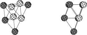
Figure 8. Defining a 2-dimensional Newton diagram as a “view” of a 3-dimensional diagram.

As $p\in{\mathcal{H}}(3,d)$, we note that the diagrams $D_{1}$ and $D_{2}$ are diagrams corresponding to polynomials in ${\mathcal{H}}(2,d)$. That is, there would be no negative terms.

We look at the 2-dimensional diagram $D_{j}$, $j=1,2$. We recall a fact noticed by D’Angelo, Kos and Riehl [DKR], that we used before. We note that there can only be two nodes on the edge $(0,b)$, otherwise the diagram could not correspond to a polynomial in ${\mathcal{H}}(2,d)$ (a negative term would appear).

By Lemma 4.2 we have the estimate $SC(D_{j})\geq\frac{d+1}{2}$. Not counting the vertex node on the edge $(0,b)$, this number drops to $\frac{d}{2}$. It is not hard to see that each face node in $D_{1}$ corresponds to a node in $D$ that does not correspond to any node in $D_{2}$. On the other hand, an edge or a vertex node in $D_{1}$ could correspond to the same node in $D$ as does an edge or a vertex node in $D_{2}$.

Hence, there must be at least $2\frac{d}{2}=d$ nodes in $D$ corresponding to monomials $x_{1}^{a}x_{2}^{b}x_{3}^{c}$ with $a\geq 1$, that is, nodes that correspond to terms that depend on the variable $x_{1}$. This completes the proof. ∎

In the case when $p$ has a monomial that depends on at most three variables we immediately obtain the sharp estimate.

Corollary 7.4.

Let $p\in{\mathcal{H}}(n,d)$, $n\geq 3$ and assume that $p$ has a monomial term of degree $d$ that depends on at most three variables. Then

$$d\leq\frac{N(p)-1}{n-1}.$$ (66)

Proof.

The statement follows by induction on $n$. When $n=3$ we have already proved the estimate. Without loss of generality assume that $p$ contains a monomial $x_{1}^{a}x_{2}^{b}x_{3}^{c}$ with $a+b+c=d$. When $n\geq 4$ we can set $x_{k}=0$ for some $k>3$. By Theorem 7.3 we lose at least $d$ terms and by the assumption that $p$ has the term $x_{1}^{a}x_{2}^{b}x_{3}^{c}$ the degree remains $d$. Applying the induction hypothesis for $n-1$ variables completes the proof. ∎

Unfortunately for a general polynomial the degree may drop when a variable is eliminated which means the proof of Corollary 7.4 does not work for all $p\in{\mathcal{H}}(n,d)$.

8. Connection to CR geometry

As we mentioned in the introduction, the primary motivation for this work comes from CR geometry. Let us describe this connection in detail.

A basic question in CR geometry is to classify CR maps $f\colon M\to M^{\prime}$ of CR manifolds $M$ and $M^{\prime}$ of possibly different dimensions. The sphere and the hyperquadrics are the simplest examples of CR manifolds. Under enough regularity assumptions, for general $M$ and $M^{\prime}$ few if any such maps exist. However, the sphere and the hyperquadrics admit a lot of symmetry that allows many inequivalent maps to exist. Much effort has been expended in the CR geometry community in understanding the case when one or both of $M$ and $M^{\prime}$ are spheres and hyperquadrics. For the sphere case, see for example [L:hq23, DLP, DKR, HJX, DAngelo:CR, D:prop1, D:poly, DL:families, DL:complex] and the references within. For the general hyperquadric case see [BH, HJX, BEH] and the references within.

First define the hyperquadric $Q(a,b)\subset{\mathbb{C}}^{n}$, where $a+b=n$, by

$$Q(a,b):=\{z\in{\mathbb{C}}^{n}\mid\sum_{k=1}^{a}\left\lvert{z_{k}}\right\rvert^{2}-\sum_{k=a+1}^{a+b}\left\lvert{z_{k}}\right\rvert^{2}=1\}.$$ (67)

Note that $Q(n,0)$ is the sphere $S^{2n-1}$. We can also regard $Q(a,b)$ as a subset of the complex projective space ${\mathbb{CP}}^{n}$ by replacing the 1 on the right hand side by $\left\lvert{z_{0}}\right\rvert^{2}$.

Given any real algebraic manifold $M\subset{\mathbb{C}}^{n}$ we can take a real polynomial $p$ vanishing on $M$ and write

$$p(z,\bar{z})=\left\lVert{f(z)}\right\rVert^{2}-\left\lVert{g(z)}\right\rVert^{2},$$ (68)

where $f$ and $g$ are mappings to some Hilbert spaces ${\mathbb{C}}^{a}$ and ${\mathbb{C}}^{b}$ and $\left\lVert{\cdot}\right\rVert$ denotes the standard Hilbert space norm on ${\mathbb{C}}^{a}$ and ${\mathbb{C}}^{b}$. If we homogenize the map $(f,g)$ we get a homogeneous polynomial map to ${\mathbb{C}}^{a+b}$. Hence $p$ gives rise to a rational CR map of $M$ to $Q(a,b-1)\subset{\mathbb{CP}}^{a+b-1}$. See [DAngelo:CR, L:hq23] for more on this construction.

When $M=M^{\prime}=S^{2n-1}\subset{\mathbb{C}}^{n}$, $n\geq 2$, then any nonconstant CR map $f$ must be a linear fractional automorphism of the unit ball [Pincuk]. Faran [Faran:B2B3] classified all sufficiently smooth maps of $S^{3}$ to $S^{5}$. The first author [L:hq23] recently finished Faran’s classification for all rational hyperquadric maps in dimensions $2$ and $3$. Forstnerič [Forstneric] proved that any $C^{\infty}$ CR map of spheres is rational and that the degree of $F$ is bounded in terms of $n$ and $N$.

When every component of a map is a single monomial, we say the map is monomial. While there exist maps that are not equivalent to monomial maps, the monomial maps are a rich subset of examples, which exhibit much of the combinatorial difficulty of the classification problem. Given a CR map $f\colon S^{2n-1}\to S^{2N-1}$ for $n\geq 3$ and the codimension $N-n$ sufficiently small, all such maps are equivalent to quadratic monomial maps. See [Faran:lin] and others, most recently [HJX]. The first author proved in [L:hq23] that all quadratic $f$ are equivalent to monomial maps. While there exist degree 3 rational maps that are not equivalent to monomial maps [FHJZ, L:hq23], all the known examples are at least homotopic to a monomial map.

D’Angelo classified the polynomial CR sphere maps [D:poly] in the following sense. If we allow the target dimension to be large enough, all polynomial proper maps are obtained by a finite number of operations from the unique homogeneous sphere map of same degree. See also the survey [Forstneric:survey] or the book [DAngelo:CR] for more information about the problem. D’Angelo conjectured that if $f\colon S^{2n-1}\to S^{2N-1}$ is a rational CR map, then

$$\deg f\leq\begin{cases}2N-3&\text{ if $n=2$}\\ \frac{N-1}{n-1}&\text{ if $n\geq 3$}\end{cases}.$$ (69)

If true, this bound is sharp; there exist maps that achieve equality in the bound. In fact, there exist monomial maps that achieve equality. No such bound exists when $n=1$; $z\mapsto z^{d}$ takes $S^{1}$ to $S^{1}$ and is of arbitrary degree.

In [DKR], D’Angelo, Kos, and Riehl proved the bound (69) for monomial maps when $n=2$. One of the main results of this paper extends their results to $n=3$.

To extend such bounds to hyperquadric maps, we need an extra condition. It is not hard to construct unbounded hyperquadric maps, for example

$$[z_{0},z_{1},z_{2}]\mapsto[z_{2}^{d-1}z_{0},z_{2}^{d-1}z_{1},z_{0}^{d},z_{0}^{d-1}z_{1},z_{2}^{d},z_{0}^{d-1}z_{2}]$$ (70)

is the homogenized rational CR map taking $S^{3}$ to $Q(4,1)$ and is of arbitrary degree $d$. We simply compose the map with the defining equation for $Q(4,1)$ in homogeneous coordinates for ${\mathbb{CP}}^{5}$ and find

$$\left\lvert{z_{2}^{d-1}z_{0}}\right\rvert^{2}+\left\lvert{z_{2}^{d-1}z_{1}}\right\rvert^{2}+\left\lvert{z_{0}^{d}}\right\rvert^{2}+\left\lvert{z_{0}^{d-1}z_{1}}\right\rvert^{2}-\left\lvert{z_{2}^{d}}\right\rvert^{2}-\left\lvert{z_{0}^{d-1}z_{2}}\right\rvert^{2}=\\ =(\left\lvert{z_{2}}\right\rvert^{2})^{d-1}(\left\lvert{z_{0}}\right\rvert^{2}+\left\lvert{z_{1}}\right\rvert^{2}-\left\lvert{z_{2}}\right\rvert^{2})+(\left\lvert{z_{0}}\right\rvert^{2})^{d-1}(\left\lvert{z_{0}}\right\rvert^{2}+\left\lvert{z_{1}}\right\rvert^{2}-\left\lvert{z_{2}}\right\rvert^{2}).$$ (71)

The map $z\mapsto[z_{2}^{d-1}z_{0},z_{2}^{d-1}z_{1},z_{2}^{d}]$ is equivalent to the map $z\mapsto[z_{0},z_{1},z_{2}]$. Similarly $z\mapsto[z_{0}^{d},z_{0}^{d-1}z_{1},z_{0}^{d-1}z_{2}]$ is also equivalent to $z\mapsto[z_{0},z_{1},z_{2}]$. Therefore, in homogeneous coordinates, the map (70) is simply the direct sum of two representatives of the linear map. And the linear map of course takes $S^{3}$ to $S^{3}$. Of course the map depends on which representatives we pick. For different representatives we get different maps. We will call maps such as the map (70) decomposable.

Definition 8.1.

A rational map $f\colon Q(a,b)\to Q(c,d)$ is said to be decomposable, if the induced homogeneous polynomial map $F$ can be decomposed as

$$F=G\oplus H,$$ (72)

where $G$ and $H$ are homogeneous polynomial maps that induce rational maps $g\colon Q(a,b)\to Q(c_{1},d_{1})$ and $h\colon Q(a,b)\to Q(c_{2},d_{2})$. If $f$ is not decomposable, it is said to be indecomposable.

If $f$ is a monomial map (that is, if we can pick homogeneous coordinates such that every component of $F$ is a monomial), and there exist monomial $G$ and $H$ as above, then $f$ is said to be monomial-decomposable. If $f$ is not monomial-decomposable, it is said to be monomial-indecomposable.

It is not hard to see that a CR map of spheres must be indecomposable. Therefore, results that apply to indecomposable hyperquadric maps in general carry over to maps of spheres.

We now connect monomial CR maps to the real algebraic setup of this paper. Suppose that a monomial CR map $f\colon Q(a,b)\to Q(c,d)$ is written in homogeneous coordinates.

$$z\mapsto[f_{1}(z),\ldots,f_{N+1}(z)].$$ (73)

As $f$ is monomial, assume that for some multi-index $\alpha_{k}$ we have

$$f_{k}(z)=C_{\alpha_{k}}z^{\alpha_{k}}.$$ (74)

Take a defining function in homogeneous coordinates for the target hyperquadric $Q(c,d)$

$$\sum_{k=1}^{c}\left\lvert{w_{k}}\right\rvert^{2}-\sum_{k=c+1}^{c+d+1}\left\lvert{w_{k}}\right\rvert^{2}.$$ (75)

Now compose $f$ with this defining function to obtain

$$\sum_{k=1}^{c}\left\lvert{f_{k}(z)}\right\rvert^{2}-\sum_{k=c+1}^{c+d+1}\left\lvert{f_{k}(z)}\right\rvert^{2}.$$ (76)

By replacing $\left\lvert{z_{0}}\right\rvert^{2}$ with $x_{0}$, $\left\lvert{z_{1}}\right\rvert^{2}$ with $x_{1}$, and so on, we obtain

$$\sum_{k=1}^{c}\left\lvert{C_{\alpha_{k}}}\right\rvert^{2}x^{\alpha_{k}}-\sum_{k=c+1}^{c+d+1}\left\lvert{C_{\alpha_{k}}}\right\rvert^{2}x^{\alpha_{k}}.$$ (77)

The defining equation for the source hyperquadric $Q(a,b)$ becomes

$$\sum_{k=1}^{a}x_{k}-\sum_{k=a+1}^{a+b+1}x_{k}.$$ (78)

Hence, (77) is zero whenever (78) is zero.

If none of the monomials of $f$ are repeated (that is if two components of $f$ are the same monomial up to a constant multiple), it is not hard to see that the degree of (77) is equal to the degree of $f$.

Proposition 8.2.

Let $f\colon Q(a,b)\to Q(c,d)$ be a monomial CR map. Suppose that the components of $f$ are linearly independent.

1. The degree of (77) is equal to the degree of $f$.

2. The map $f$ is monomial-indecomposable if and only if (77) is indecomposable in the sense of Definition 2.1.

Proof.

To prove (i), notice that for a monomial map the components of $f$ are linearly independent if and only if no monomial of $f$ is repeated. Then it is obvious that the degree of $f$ must be equal to the degree of the induced polynomial (77).

To prove (ii), notice that as the components of $f$ are linearly independent, each component of $f$ produces a different monomial in (77). The statement follows. ∎

Using Proposition 8.2 we can apply results of this paper to monomial CR maps of hyperquadrics. Therefore the proof of Theorem 1.3 is a trivial application of this Proposition and the results of this paper. In particular, part (i) of Theorem 1.3 follows by Theorem 2.4, part (ii) follows by Theorem 1.2, and finally part (iii) follows by Theorem 7.2.

Therefore, at least for monomial maps, indecomposability appears to be the correct condition to require to obtain degree bounds for general hyperquadric maps.