Classical Strongly Coupled QGP:
VII. Shear Viscosity and Self Diffusion

Abstract

We construct the Liouville operator for the SU(2) classical colored Coulomb plasma (cQGP) for arbitrary values of the Coulomb coupling $\Gamma=V/K$, the ratio of the mean Coulomb to kinetic energy. We show that its resolvent in the classical colored phase space obeys a hierarchy of equations. We use a free streaming approximation to close the hierarchy and derive an integral equation for the time-dependent structure factor. Its reduction by projection yields hydrodynamical equations in the long-wavelength limit. We discuss the character of the hydrodynamical modes at strong coupling. The shear viscosity is shown to exhibit a minimum at $\Gamma\approx 8$ near the liquid point. This minimum follows from the cross-over between the single particle collisional regime which drops as $1/\Gamma^{5/2}$ and the hydrodynamical collisional regime which rises as $\Gamma^{1/2}$. The self-diffusion constant drops as $1/\Gamma^{3/2}$ irrespective of the regime. We compare our results to molecular dynamics simulations of the SU(2) colored Coulomb plasma. We also discuss the relevance of our results for the quantum and strongly coupled quark gluon plasma (sQGP).

I Introduction

High temperature QCD is expected to asymptote a weakly coupled Coulomb plasma albeit with still strong infrared divergences. The latters cause its magnetic sector to be non-perturbative at all temperatures. At intermediate temperatures of relevance to heavy-ion collider experiments, the electric sector is believed to be strongly coupled.

Recently, Shuryak and Zahed SZ_newqgp have suggested that certain aspects of the quak-gluon plasma in range of temperatures $(1-3)\,T_{c}$ can be understood by a stronger Coulomb interaction causing persistent correlations in singlet and colored channels. As a result the quark and gluon plasma is more a liquid than a gas at intermediate temperatures. A liquid plasma should exhibit shorter mean-free paths and stronger color dissipation, both of which are supported by the current experiments at RHIC hydro .

To help understand transport and dissipation in the strongly coupled quark gluon plasma, a classical model of the colored plasma was suggested in gelmanetal . The model consists of massive quarks and gluons interacting via classical colored Coulomb interactions. The color is assumed classical with all equations of motion following from Poisson brackets. For the SU(2) version both molecular dynamics simulations gelmanetal and bulk thermodynamics cho&zahed ; cho&zahed2 were recently presented including simulations of the energy loss of heavy quarks dusling&zahed .

In this paper we extend our recent equilibrium analysis of the static properties of the colored Coulomb plasma, to transport. In section 2 we discuss the classical equations of motion in the SU(2) colored phase space and derive the pertinent Liouville operator. In section 3, we show that the resolvent of the Liouville operator obeys a hierarchy of equations in the SU(2) phase space. In section 4 we derive an integral equation for the time-dependent structure factor by introducing a non-local self-energy kernel in phase space. In section 5, we close the Liouville hierarchy through a free streaming approximation on the 4-point resolvent and derive the self-energy kernel in closed form. In section 6, we project the self-energy kernel and the non-static structure factor onto the colorless hydrodynamical phase space. In section 7, we show that the sound and plasmon mode are the leading hydrodynamical modes in the SU(2) colored Coulomb plasma. In section we analyze the shear viscosity for the transverse sound mode for arbitrary values of $\Gamma$. We show that a minimum forms at $\Gamma\approx 5$ at the cross-over between the hydrodynamical and single-particle regimes. In section 8, we analyze self-diffusion in phase space, and derive an explicit expression for the diffusion constant at strong coupling. Our conclusions and prospects are in section 9. In appendix A we briefly summarize our variables in the SU(2) phase space. In appendix B we detail the projection method for the self-energy kernel used in the text. In appendix C we show that the collisional color contribution to the Liouville operator drops in the self-energy kernel. In appendix D some useful aspects of the hydrodynamical projection method are outlined.

II Colored Liouville Operator

The canonical approach to the colored Coulomb plasma was discussed in gelmanetal . In brief, the Hamiltonian for a single species of constituent quarks or gluons in the SU(2) representation is defined as

$$H=\sum_{i}^{N}\frac{\boldsymbol{p}^{2}_{i}}{2m_{i}}+\sum_{i>j=1}^{N}\frac{\boldsymbol{Q}_{i}\cdot\boldsymbol{Q}_{j}}{|\boldsymbol{r}_{i}-\boldsymbol{r}_{j}|}$$ (II.1)

The charge $g^{2}/4\pi$ has been omitted for simplicity of the notation flow and will be reinserted in the pertinent physical quantities by inspection.

The equations of motion in phase space follows from the classical Poisson brackets. In particular

$$\frac{d\boldsymbol{r}_{i}}{dt}=-\{H,\boldsymbol{r}_{i}\}=\frac{\partial H}{\partial\boldsymbol{p}_{j}}\frac{\partial\boldsymbol{r}_{i}}{\partial\boldsymbol{r}_{j}}=\frac{\boldsymbol{p}_{i}}{m}$$ (II.2)

The Newtonian equation of motion is just the colored electric Lorentz force

$$\frac{d\boldsymbol{p}_{i}}{dt}=-\{H,\boldsymbol{p}_{i}\}=-\frac{\partial H}{\partial\boldsymbol{r}_{j}}\frac{\partial\boldsymbol{p}_{i}}{\partial\boldsymbol{p}_{j}}=Q_{i}^{a}\,\boldsymbol{E}_{i}^{a}=\boldsymbol{F}_{i}$$ (II.3)

with the colored electric field and potentials defined as ($a=1,2,3$)

$$\boldsymbol{E}_{i}^{a}=-\boldsymbol{\nabla}_{i}\Phi^{a}_{i}=-\boldsymbol{\nabla}_{i}\sum_{j\neq i}\frac{Q^{a}_{j}}{|\boldsymbol{r}_{i}-\boldsymbol{r}_{j}|}$$ (II.4)

Our strongly coupled colored plasma is mostly electric following the original assumptions in gelmanetal ; gelmanetal2 . The equation of motion of the color charges is

$$\frac{dQ_{i}^{a}}{dt}=-\{H,Q_{i}^{a}\}=-\sum_{j,b}\frac{\partial H}{\partial Q_{i}^{b}}\frac{\partial Q_{i}^{a}}{\partial Q_{j}^{c}}\{Q_{j}^{b},Q_{j}^{c}\}=\sum_{j\neq i}\frac{Q_{i}T^{a}Q_{j}}{|\boldsymbol{r}_{i}-\boldsymbol{r}_{j}|}$$ (II.5)

for arbitrary color representation. For SU(2) the classical color charge (II.5) precesses around the net colored potential $\Phi$ determined by the other particles as defined in (II.4),

$$\frac{d\boldsymbol{Q}_{i}}{dt}=(\boldsymbol{\Phi}_{i}\times\boldsymbol{Q}_{i})$$ (II.6)

This equation was initially derived by Wong wong . Some aspects of the SU(2) phase space are briefly recalled in Appendix A.

The set (II.2), (II.3) and (II.5) define the canonical evolution in phase space. The time-dependent phase distribution is formally given by

$$f(t,\boldsymbol{r}\boldsymbol{p}\boldsymbol{Q})=\sum_{i=1}^{N}\delta(\boldsymbol{r}-\boldsymbol{r}_{i}(t))\delta(\boldsymbol{p}-\boldsymbol{p}_{i}(t))\delta(\boldsymbol{Q}-\boldsymbol{Q}_{i}(t))\equiv\sum_{i}\delta(\boldsymbol{q}-\boldsymbol{q}_{i}(t))$$ (II.7)

For simplicity $\boldsymbol{q}$ is generic for $\boldsymbol{r},\boldsymbol{p},\boldsymbol{Q}$. Using the chain rule, the time-evolution operator on (II.7) obeys

$$\frac{d}{dt}=\frac{\partial}{\partial t}+\frac{d\boldsymbol{r}_{i}}{dt}\frac{\partial}{\partial\boldsymbol{r}_{i}}+\frac{d\boldsymbol{p}_{i}}{dt}\frac{\partial}{\partial\boldsymbol{p}_{i}}+\frac{d\boldsymbol{Q}_{i}}{dt}\frac{\partial}{\partial\boldsymbol{Q}_{i}}\equiv\partial_{t}+i\mathcal{L}$$ (II.8)

The last relation defines the Liouville operator

$$\mathcal{L}=\mathcal{L}_{0}+\mathcal{L}_{I}+\mathcal{L}_{Q}=-i\boldsymbol{v}_{i}\cdot\nabla_{\boldsymbol{r}_{i}}-i\,\boldsymbol{F}_{i}\cdot\boldsymbol{\nabla}_{\boldsymbol{p}_{i}}-i\boldsymbol{\Phi}_{i}\cdot(\boldsymbol{Q}_{i}\times\boldsymbol{\nabla}_{\boldsymbol{Q}_{i}})$$ (II.9)

The last contribution in (II.9) is genuily a 3-body force because of the cross product (orbital color operator). It requires 3 distinct colors to not vanish. This observation will be important in simplifying the color dynamics below. Also (II.9) is hermitean.

Since (II.7) depends implicitly on time, we can write formally

$$\frac{d}{dt}f(t,\boldsymbol{r}\boldsymbol{p}\boldsymbol{Q})=i\mathcal{L}f(t,\boldsymbol{r}\boldsymbol{p}\boldsymbol{Q})$$ (II.10)

with a solution $f(t)=e^{i\mathcal{L}t}f(0)$. The formal relation (II.10) should be considered with care since the action of the Liouville operator on the 1-body phase space distribution (II.7) generates also a 2-body phase space distribution. Indeed, while $\mathcal{L}_{0}$ is local in phase space

$$\mathcal{L}_{0}\sum_{i}\delta(\boldsymbol{q}-\boldsymbol{q}_{i})=-i\boldsymbol{v}\cdot\nabla_{\boldsymbol{r}}\sum_{i}\delta(\boldsymbol{q}-\boldsymbol{q}_{i})=L_{0}(\boldsymbol{q})\sum_{i}\delta(\boldsymbol{q}-\boldsymbol{q}_{i})$$ (II.11)

the 2 other contributions are not. Specifically

$$\mathcal{L}_{I}\sum_{m}\delta(\boldsymbol{q}-\boldsymbol{q}_{m}) = i\sum_{i\neq j}\nabla_{\boldsymbol{r}_{i}}\frac{\boldsymbol{Q}_{i}\cdot\boldsymbol{Q}_{j}}{|\boldsymbol{r}_{i}-\boldsymbol{r}_{j}|}\cdot\nabla_{\boldsymbol{p}_{i}}\sum_{m}\delta(\boldsymbol{q}-\boldsymbol{q}_{m})$$ (II.12)

$$= i\int d\boldsymbol{q}^{\prime}\sum_{i\neq j,mn}\nabla_{\boldsymbol{r}_{i}}\frac{\boldsymbol{Q}_{i}\cdot\boldsymbol{Q}_{j}}{|\boldsymbol{r}_{i}-\boldsymbol{r}_{j}|}\cdot\nabla_{\boldsymbol{p}_{i}}\,\,\delta(\boldsymbol{q}-\boldsymbol{q}_{m})\delta(\boldsymbol{q}^{\prime}-\boldsymbol{q}_{n})$$

$$= -\int d\boldsymbol{q}^{\prime}L_{I}(\boldsymbol{q},\boldsymbol{q}^{\prime})\,\sum_{mn}\delta(\boldsymbol{q}-\boldsymbol{q}_{m})\delta(\boldsymbol{q}^{\prime}-\boldsymbol{q}_{n})$$

with

$$L_{I}(\boldsymbol{q},\boldsymbol{q}^{\prime})=i\nabla_{\boldsymbol{r}}\frac{\boldsymbol{Q}\cdot\boldsymbol{Q}^{\prime}}{|\boldsymbol{r}-\boldsymbol{r}^{\prime}|}\cdot(\nabla_{\boldsymbol{p}}-\nabla_{\boldsymbol{p}^{\prime}})$$ (II.13)

Similarly

$$\mathcal{L}_{Q}\sum_{m}\delta(\boldsymbol{q}-\boldsymbol{q}_{m}) = -i\sum_{j\neq i,m}\frac{\boldsymbol{Q}_{i}\times\boldsymbol{Q}_{j}}{|\boldsymbol{r}_{i}-\boldsymbol{r}_{j}|}\cdot\nabla_{\boldsymbol{Q}_{i}}\,\delta(\boldsymbol{q}-\boldsymbol{q}_{m})$$ (II.14)

$$= -i\int d\boldsymbol{q}^{\prime}\sum_{j\neq i,mn}\frac{\boldsymbol{Q}_{i}\times\boldsymbol{Q}_{j}}{|\boldsymbol{r}_{i}-\boldsymbol{r}_{j}|}\cdot\nabla_{\boldsymbol{Q}_{i}}\delta(\boldsymbol{q}-\boldsymbol{q}_{m})\delta(\boldsymbol{q}^{\prime}-\boldsymbol{q}_{n})$$

$$= -\int d\boldsymbol{q}^{\prime}L_{Q}(\boldsymbol{q},\boldsymbol{q}^{\prime})\sum_{mn}\delta(\boldsymbol{q}-\boldsymbol{q}_{m})\delta(\boldsymbol{q}^{\prime}-\boldsymbol{q}_{n})$$

with

$$L_{Q}(\boldsymbol{q},\boldsymbol{q}^{\prime})=-i\frac{\boldsymbol{Q}\times\boldsymbol{Q}^{\prime}}{|\boldsymbol{r}-\boldsymbol{r}^{\prime}|}\cdot(\nabla_{\boldsymbol{Q}}-\nabla_{\boldsymbol{Q}^{\prime}})$$ (II.15)

Clearly (II.14) drops from 2-body and symmetric phase space distributions. It does not for 3-body and higher.

III Liouville Hierarchy

An important correlation function in the analysis of the colored Coulomb plasma is the time dependent structure factor or 2-body correlation in the color phase space

$${\bf S}(t-t^{\prime},\boldsymbol{r}-\boldsymbol{r}^{\prime},\boldsymbol{p}\boldsymbol{p}^{\prime},\boldsymbol{Q}\cdot\boldsymbol{Q}^{\prime})=\langle\delta f(t,\boldsymbol{r}\boldsymbol{p}\boldsymbol{Q})\,\delta f(t^{\prime},\boldsymbol{r}^{\prime}\boldsymbol{p}^{\prime}\boldsymbol{Q}^{\prime})\rangle$$ (III.1)

with $\delta f=f-\langle f\rangle$ the shifted 1-body phase space distribution. The averaging in (III.1) is carried over the initial conditions with fixed number of particles $N$ and average energy or temperature $\beta=1/T$. Thus $\langle f\rangle=nf_{0}(p)$ which is the Maxwellian distribution for constituent quarks or gluons. In equilibrium, the averaging in (III.1) is time and space translational invariant as well as color rotational invariant.

Using the ket notation with $\boldsymbol{1}\equiv\boldsymbol{q}\equiv{\boldsymbol{r}}{\boldsymbol{p}}{\boldsymbol{Q}}$

$$|\delta f(t,\boldsymbol{1})\rangle=\bigg{|}\sum_{m}\delta(\boldsymbol{q}-\boldsymbol{q}_{m}(t))-\langle\sum_{m}\delta(\boldsymbol{q}-\boldsymbol{q}_{m}(t))\bigg{\rangle}\equiv|\delta f(t,\boldsymbol{1})-\langle f(t,\boldsymbol{1})\rangle>$$ (III.2)

with also $\boldsymbol{2}=\boldsymbol{q}^{\prime}$, $\boldsymbol{3}=\boldsymbol{q}^{\prime\prime}$, $\boldsymbol{4}=\boldsymbol{q}^{\prime\prime\prime}$ and so on and the formal Liouville solution $\delta f(t,\boldsymbol{1})=e^{i\mathcal{L}t}\delta f(\boldsymbol{1})$ we can write (III.1) as

$${\bf S}(t-t^{\prime},\boldsymbol{q},\boldsymbol{q}^{\prime})=\langle\delta f(t,\boldsymbol{1})|\delta f(t^{\prime},\boldsymbol{2})\rangle=\langle\delta f(\boldsymbol{1})|e^{i{\cal L}(t^{\prime}-t)}|\delta f(\boldsymbol{2})\rangle$$ (III.3)

The bra-ket notation is short for the initial or equilibrium average. Its Laplace or causal transform reads

$${\bf S}(z,\boldsymbol{q},\boldsymbol{q}^{\prime})=-i\int_{-\infty}^{+\infty}\,dt\,\,\theta(t-t^{\prime})\,\,e^{izt}\,\,{\bf S}(t-t^{\prime},\boldsymbol{q},\boldsymbol{q}^{\prime})=\langle\delta f(\boldsymbol{1})|\frac{1}{z+\mathcal{L}}|\delta f(\boldsymbol{2})\rangle$$ (III.4)

with $z=\omega+i0$. Clearly

$$z{\bf S}(z,\boldsymbol{q},\boldsymbol{q}^{\prime})+\langle\delta f(\boldsymbol{1})|\mathcal{L}\frac{1}{z+\mathcal{L}}|\delta f(\boldsymbol{2})\rangle=\langle\delta f(\boldsymbol{1})|\delta f(\boldsymbol{2})\rangle$$ (III.5)

Since ${\cal L}^{\dagger}={\cal L}$ is hermitian and using (II.11), (II.12) and (II.14) it follows that

$$\langle\delta f(\boldsymbol{1})|{\cal L}=\langle\delta f(\boldsymbol{1})|{L}_{0}(\boldsymbol{q})-\int\,d\boldsymbol{q}"\,L_{I+Q}(\boldsymbol{q},\boldsymbol{q}^{\prime\prime})\,\langle\delta f(\boldsymbol{1})\delta f(\boldsymbol{3})|$$ (III.6)

Thus

$$\Big{(}z-L_{0}(\boldsymbol{q})\Big{)}{\bf S}(z,\boldsymbol{q},\boldsymbol{q}^{\prime})-\int\,d\boldsymbol{q}^{\prime\prime}L_{I+Q}(\boldsymbol{q}^{\prime},\boldsymbol{q}^{\prime\prime}){\bf S}(z,\boldsymbol{q}\boldsymbol{q}^{\prime\prime},\boldsymbol{q}^{\prime})={\bf S}_{0}(\boldsymbol{q},\boldsymbol{q}^{\prime})$$ (III.7)

where we have defined the 3-body phase space resolvent

$${\bf S}(z,\boldsymbol{q}\boldsymbol{q}^{\prime\prime},\boldsymbol{q}^{\prime})=\,\langle\delta f(\boldsymbol{1})\delta f(\boldsymbol{3})|\frac{1}{z+{\cal L}}\,|\delta f(\boldsymbol{2})>$$ (III.8)

${\bf S}_{0}(\boldsymbol{q},\boldsymbol{q}^{\prime})$ is the static colored structure factor discussed by us in cho&zahed3 . Since $L_{I+Q}(\boldsymbol{q}^{\prime},\boldsymbol{q})$ is odd under the switch $\boldsymbol{q}\leftrightarrow\boldsymbol{q}^{\prime}$, and since ${\bf S}(z,\boldsymbol{q}\boldsymbol{q}^{\prime\prime},\boldsymbol{q}^{\prime})={\bf S}(-z,\boldsymbol{q},\boldsymbol{q}^{\prime}\boldsymbol{q}^{\prime\prime})$ owing to the $t\leftrightarrow t^{\prime}$ in (III.4), then

$$\Big{(}z+L_{0}(\boldsymbol{q}^{\prime})\Big{)}{\bf S}(z,\boldsymbol{q},\boldsymbol{q}^{\prime})-\int\,d\boldsymbol{q}^{\prime\prime}L_{I+Q}(\boldsymbol{q}^{\prime},\boldsymbol{q}^{\prime\prime}){\bf S}(z,\boldsymbol{q},\boldsymbol{q}^{\prime}\boldsymbol{q}^{\prime\prime})={\bf S}_{0}(\boldsymbol{q},\boldsymbol{q}^{\prime})$$ (III.9)

(III.7) or equivalently (III.9) define the Liouville hierarchy, whereby the 2-body phase space distribution ties to the 3-body phase space distribution and so on. Indeed, (III.9) for instance implies

$$\Big{(}z+L_{0}(\boldsymbol{q}^{\prime\prime})\Big{)}{\bf S}(z,\boldsymbol{q}\boldsymbol{q}^{\prime},\boldsymbol{q}^{\prime\prime})-\int\,d\boldsymbol{q}^{\prime\prime\prime}L_{I+Q}(\boldsymbol{q}^{\prime\prime},\boldsymbol{q}^{\prime\prime\prime}){\bf S}(z,\boldsymbol{q}\boldsymbol{q}^{\prime},\boldsymbol{q}^{\prime\prime}\boldsymbol{q}^{\prime\prime\prime})={\bf S}_{0}(\boldsymbol{q}\boldsymbol{q}^{\prime},\boldsymbol{q}^{\prime\prime})$$ (III.10)

with the 4-point resolvent function

$${\bf S}(z,\boldsymbol{q}\boldsymbol{q}^{\prime},\boldsymbol{q}^{\prime\prime}\boldsymbol{q}^{\prime\prime\prime})=\,\langle\delta f(\boldsymbol{1})\delta f(\boldsymbol{2})|\frac{1}{z+{\cal L}}\,|\delta f(\boldsymbol{3})\delta f(\boldsymbol{4})>$$ (III.11)

These are the microscopic kinetic equations for the color phase space distributions. They are only useful when closed, that is by a truncation as we discuss below. These formal equations where initially discussed in foster&martin ; foster ; mazenko1 ; mazenko3 in the context of the one component Coulomb Abelian Coulomb plasma. We have now generalized them to the multi-component and non-Abelian colored Coulomb plasma.

IV Self-Energy Kernel

In (III.7) the non-local part of the Liouville operator plays the role of a non-local self-energy kernel $\Sigma$ on the 2-body resolvent. Indeed, we can rewrite (III.7) as

$$(z-L_{0}(\boldsymbol{q})){\bf S}(z,\boldsymbol{q},\boldsymbol{q}^{\prime})-\int dq^{\prime\prime}\Sigma(z,\boldsymbol{q},\boldsymbol{q}^{\prime\prime}){\bf S}(z,\boldsymbol{q}^{\prime\prime},\boldsymbol{q}^{\prime})={\bf S}_{0}(\boldsymbol{q},\boldsymbol{q}^{\prime})$$ (IV.1)

with the non-local self-energy kernel defined formally as

$$\int d\boldsymbol{q}^{\prime\prime}\Sigma(z,\boldsymbol{q},\boldsymbol{q}^{\prime\prime})\,{\bf S}(z,\boldsymbol{q}^{\prime\prime},\boldsymbol{q}^{\prime})=\int d\boldsymbol{q}^{\prime\prime}L_{I+Q}(\boldsymbol{q},\boldsymbol{q}^{\prime\prime})\,{\bf S}(z,\boldsymbol{q}\boldsymbol{q}^{\prime\prime},\boldsymbol{q}^{\prime})$$ (IV.2)

The self-energy kernel $\Sigma$ can be regarded as the sum of a static or z-independent contribution $\Sigma_{S}$ ans a non-static or collisional contribution $\Sigma_{C}$,

$$\Sigma(z,\boldsymbol{q},\boldsymbol{q}^{\prime\prime})=\Sigma_{S}(\boldsymbol{q},\boldsymbol{q}^{\prime\prime})+\Sigma_{C}(z,\boldsymbol{q},\boldsymbol{q}^{\prime\prime})$$ (IV.3)

The stationary part $\Sigma_{S}$ satisfies

$$\int d\boldsymbol{q}^{\prime\prime}\Sigma_{S}(\boldsymbol{q},\boldsymbol{q}^{\prime\prime})\,{\bf S}_{0}(\boldsymbol{q}^{\prime\prime},\boldsymbol{q}^{\prime})=\int d\boldsymbol{q}^{\prime\prime}L_{I+Q}(\boldsymbol{q},\boldsymbol{q}^{\prime\prime})\,{\bf S}_{0}(\boldsymbol{q},\boldsymbol{q}^{\prime},\boldsymbol{q}^{\prime\prime})$$ (IV.4)

which identifies it with the sum of the 2- and 3-body part of the Liouville operator $L_{I+Q}$.

The collisional part $\Sigma_{C}$ is more involved. To unwind it, we operate with $(z+L_{0}(\boldsymbol{q}^{\prime}))$ on both sides of (IV.2), and then reduce the left hand side contribution using (III.9) and the right hand side contribution using (III.10). The outcome reduces to

$$\Sigma_{C}(z,\boldsymbol{q},\boldsymbol{q}^{\prime\prime})\,{\bf S}_{0}(\boldsymbol{q}^{\prime\prime},\boldsymbol{q}^{\prime})= -\int d\boldsymbol{q}^{\prime\prime\prime}\,L_{I+Q}(\boldsymbol{q},\boldsymbol{q}^{\prime\prime})L_{I+Q}(\boldsymbol{q}^{\prime},\boldsymbol{q}^{\prime\prime})\,{\bf S}(z,\boldsymbol{q}\boldsymbol{q}^{\prime\prime},\boldsymbol{q}^{\prime}\boldsymbol{q}^{\prime\prime\prime})$$ (IV.5)

$$+\int\,dq^{\prime\prime\prime}\,\Sigma(z,\boldsymbol{q},\boldsymbol{q}^{\prime\prime})\,L_{I+Q}(\boldsymbol{q}^{\prime},\boldsymbol{q}^{\prime\prime})\,{\bf S}(z,\boldsymbol{q}^{\prime\prime},\boldsymbol{q}^{\prime}\boldsymbol{q}^{\prime\prime\prime})$$

after using (IV.4). From (IV.2) it follows formally that

$$\Sigma(z,\boldsymbol{q},\boldsymbol{q}^{\prime\prime})=\int\,d\boldsymbol{q}^{\prime\prime\prime}\,L_{I+Q}(\boldsymbol{q},\boldsymbol{q}^{\prime\prime\prime})\,{\bf S}^{-1}(z,\boldsymbol{q}^{\prime},\boldsymbol{q}^{\prime\prime})\,{\bf S}(z,\boldsymbol{q}\boldsymbol{q}^{\prime\prime\prime},\boldsymbol{q}^{\prime})$$ (IV.6)

Inserting (IV.6) into the right hand side of (IV.5) and taking the $\boldsymbol{q}^{\prime}$ integration on both sides yield

$$nf_{0}(p^{\prime\prime})\,\Sigma_{C}(z,\boldsymbol{q},\boldsymbol{q}^{\prime\prime})=-\int d\boldsymbol{q}^{\prime\prime}d\boldsymbol{q}^{\prime\prime\prime}\,L_{I+Q}(\boldsymbol{q},\boldsymbol{q}^{\prime\prime})L_{I+Q}(\boldsymbol{q}^{\prime},\boldsymbol{q}^{\prime\prime\prime})\,{\bf G}(z,\boldsymbol{q}\boldsymbol{q}^{\prime\prime},\boldsymbol{q}^{\prime}\boldsymbol{q}^{\prime\prime\prime})$$ (IV.7)

with ${\bf G}$ a 4-point phase space correlation function

$${\bf G}(z,\boldsymbol{q}\boldsymbol{q}_{1}^{\prime},\boldsymbol{q}^{\prime}\boldsymbol{q}_{2}^{\prime})={\bf S}(z,\boldsymbol{q}\boldsymbol{q}_{1}^{\prime},\boldsymbol{q}^{\prime}\boldsymbol{q}_{2}^{\prime})-\int d\boldsymbol{q}_{3}d\boldsymbol{q}_{4}{\bf S}(z,\boldsymbol{q}\boldsymbol{q}_{1}^{\prime},\boldsymbol{q}_{3}){\bf S}^{-1}(z,\boldsymbol{q}_{3},\boldsymbol{q}_{4}){\bf S}(z,\boldsymbol{q}_{4},\boldsymbol{q}^{\prime}\boldsymbol{q}_{2}^{\prime})$$ (IV.8)

The collisional character of the self-energy $\Sigma_{C}$ is manifest in (IV.7). The formal relation for the collisional self-energy (IV.7) was initially derived in mazenko1 ; mazenko3 for the one-component and Abelian Coulomb plasma. We now have shown that it holds for any non-Abelian SU(N) Coulomb plasma.

Eq. (IV.7) shows that the connected part of the self-energy kernel is actually tied to a 4-point correlator in the colored phase space. In terms of (IV.7), the original kinetic equation (III.7) now reads

$$\Big{(}z-L_{0}(\boldsymbol{q})\Big{)}{\bf S}(z,\boldsymbol{q},\boldsymbol{q}^{\prime})-\int\,d\boldsymbol{q}^{\prime\prime}\Sigma_{S}(\boldsymbol{q},\boldsymbol{q}^{\prime\prime}){\bf S}(z,\boldsymbol{q}^{\prime\prime},\boldsymbol{q}^{\prime})={\bf S}_{0}(\boldsymbol{q},\boldsymbol{q}^{\prime})$$

$$-\int\,d\boldsymbol{q}^{\prime\prime}\,d\boldsymbol{q}_{1}d\boldsymbol{q}_{2}\,L_{I+Q}(\boldsymbol{q},\boldsymbol{q}_{1})L_{I+Q}(\boldsymbol{q}^{\prime\prime},\boldsymbol{q}_{2})\,{\bf G}(z,\boldsymbol{q}\boldsymbol{q}_{1},\boldsymbol{q}^{\prime\prime}\boldsymbol{q}_{2})\,{\bf S}(z,\boldsymbol{q}^{\prime\prime},\boldsymbol{q}^{\prime})$$ (IV.9)

which is a Boltzman-like equation. The key difference is that it involves correlation functions and the Boltzman-like kernel in the right-hand side is not a scattering amplitude but rather a reduced 4-point correlation function. (IV.9) reduces to the Boltzman equation for weak coupling. An alternative derivation of (IV.9) can be found in Appendix C through a direct projection of (IV.2) in phase space.

V Free Streaming Approximation

The formal kinetic equation (IV.7) can be closed by approximating the 4-point correlation function in the color phase space by a product of 2-point correlation function mazenko3 ,

$${\bf G}(t,\boldsymbol{q}\boldsymbol{q}_{1},\boldsymbol{q}^{\prime}\boldsymbol{q}_{2})\approx\Big{(}{\bf S}(t,\boldsymbol{q},\boldsymbol{q}^{\prime}){\bf S}(t,\boldsymbol{q}_{1},\boldsymbol{q}_{2})+{\bf S}(t,\boldsymbol{q},\boldsymbol{q}_{2}){\bf S}(t,\boldsymbol{q}^{\prime},\boldsymbol{q}_{1})\Big{)}$$ (V.1)

This reduction will be referred to as the free steaming approximation. Next we substitue the colored Coulomb potentials in the double Liouville operator $L_{1+Q}\times L_{1+Q}$ with a bare Coulomb ${\bf V}(\boldsymbol{r}-\boldsymbol{r}^{\prime},\boldsymbol{Q}\cdot\boldsymbol{Q}^{\prime})=\boldsymbol{Q}\cdot\boldsymbol{Q}^{\prime}/|\boldsymbol{r}-\boldsymbol{r}^{\prime}|$.

$$L_{I+Q}(\boldsymbol{q},\boldsymbol{q}_{1})=i\nabla_{\boldsymbol{r}}{\bf V}(\boldsymbol{r}-\boldsymbol{r}_{1},\boldsymbol{Q}\cdot\boldsymbol{Q}_{1})\cdot(\nabla_{\boldsymbol{p}}-\nabla_{\boldsymbol{p}_{1}})$$

$$-i\Big{(}\boldsymbol{Q}\times\nabla_{\boldsymbol{Q}}{\bf V}(\boldsymbol{r}-\boldsymbol{r}_{1},\boldsymbol{Q}\cdot\boldsymbol{Q}_{1})\cdot\nabla_{\boldsymbol{Q}}+\boldsymbol{Q}_{1}\times\nabla_{\boldsymbol{Q}_{1}}{\bf V}(\boldsymbol{r}-\boldsymbol{r}_{1},\boldsymbol{Q}\cdot\boldsymbol{Q}_{1})\cdot\nabla_{Q_{1}}\Big{)}$$ (V.2)

times a dressed colored Coulomb potential ${\bf c}_{D}$ defined in cho&zahed3

$$L_{I+Q}^{R}(\boldsymbol{q},\boldsymbol{q}_{1})=-i\frac{1}{\beta}\nabla_{\boldsymbol{r}}{\bf c}_{D}(\boldsymbol{r}-\boldsymbol{r}_{1},\boldsymbol{Q}\cdot\boldsymbol{Q}_{1})\cdot(\nabla_{\boldsymbol{p}}-\nabla_{\boldsymbol{p}_{1}})$$

$$+i\frac{1}{\beta}\Big{(}\boldsymbol{Q}\times\nabla_{\boldsymbol{Q}}{\bf c}_{D}(\boldsymbol{r}-\boldsymbol{r}_{1},\boldsymbol{Q}\cdot\boldsymbol{Q}_{1})\cdot\nabla_{\boldsymbol{Q}}+\boldsymbol{Q}_{1}\times\nabla_{\boldsymbol{Q}_{1}}{\bf c}_{D}(\boldsymbol{r}-\boldsymbol{r}_{1},\boldsymbol{Q}\cdot\boldsymbol{Q}_{1})\cdot\nabla_{Q_{1}}\Big{)}$$ (V.3)

This bare-dressed or half renormalization was initially suggested wallenborn&baus in the context of the one-component Coulomb plasma to overcome the shortcomings of a full or dressed-dressed renormalization initially suggested in mazenko1 ; mazenko3 . The latter was shown to upset the initial conditions. Thus

$$L_{I+Q}(\boldsymbol{q},\boldsymbol{q}_{1})L_{I+Q}(\boldsymbol{q}^{\prime},\boldsymbol{q}_{2})\rightarrow\frac{1}{2}\Big{(}L_{I+Q}(\boldsymbol{q},\boldsymbol{q}_{1})L_{I+Q}^{R}(\boldsymbol{q}^{\prime},\boldsymbol{q}_{2})+L_{I+Q}^{R}(\boldsymbol{q},\boldsymbol{q}_{1})L_{I+Q}(\boldsymbol{q}^{\prime},\boldsymbol{q}_{2})\Big{)}$$ (V.4)

Combining (V.1) and (V.4) in (IV.7) yields

$$n\,f_{0}(\boldsymbol{p}^{\prime})\,\Sigma_{C}(t,\boldsymbol{q},\boldsymbol{q}^{\prime})\approx-\frac{1}{2}\int d\boldsymbol{q}_{1}\,d\boldsymbol{q}_{2}\,\bigg{(}L_{I+Q}(\boldsymbol{q},\boldsymbol{q}_{1})L_{I+Q}^{R}(\boldsymbol{q}^{\prime},\boldsymbol{q}_{2}){\bf S}(t,\boldsymbol{q},\boldsymbol{q}^{\prime}){\bf S}(t,\boldsymbol{q}_{1},\boldsymbol{q}_{2})$$

$$+L_{I+Q}(\boldsymbol{q},\boldsymbol{q}_{1})L_{I+Q}^{R}(\boldsymbol{q}^{\prime},\boldsymbol{q}_{2}){\bf S}(t,\boldsymbol{q},\boldsymbol{q}_{2}){\bf S}(t,\boldsymbol{q}^{\prime},\boldsymbol{q}_{1})+(\boldsymbol{q}_{1}\leftrightarrow\boldsymbol{q}_{2},\boldsymbol{q}\leftrightarrow\boldsymbol{q}^{\prime})\bigg{)}$$ (V.5)

This is the half dressed but free streaming approximation for the connected part of the self-energy for the colored Coulomb plasma. Translational invariance in space and rotational invariance in color space allows a further reduction of (V.5) by Fourier and Legendre transforms respectively. Indeed, Eq. (V.5) yields

$$n\,f_{0}(\boldsymbol{p}^{\prime})\,\Sigma_{C}(t,\boldsymbol{q},\boldsymbol{q}^{\prime})$$

$$\approx-\frac{1}{2}\int d\boldsymbol{q}_{1}\,d\boldsymbol{q}_{2}\,\bigg{(}L_{I}(\boldsymbol{q},\boldsymbol{q}_{1})L_{I}^{R}(\boldsymbol{q}^{\prime},\boldsymbol{q}_{2}){\bf S}(t,\boldsymbol{q},\boldsymbol{q}^{\prime}){\bf S}(t,\boldsymbol{q}_{1},\boldsymbol{q}_{2})$$

$$+L_{I}(\boldsymbol{q},\boldsymbol{q}_{1})L_{I}^{R}(\boldsymbol{q}^{\prime},\boldsymbol{q}_{2}){\bf S}(t,\boldsymbol{q},\boldsymbol{q}_{2}){\bf S}(t,\boldsymbol{q}^{\prime},\boldsymbol{q}_{1})+(\boldsymbol{q}_{1}\leftrightarrow\boldsymbol{q}_{2},\boldsymbol{q}\leftrightarrow\boldsymbol{q}^{\prime})\bigg{)}$$

$$=-\frac{1}{2\beta}\int d\boldsymbol{q}_{1}\,d\boldsymbol{q}_{2}\,\bigg{(}\nabla_{\boldsymbol{r}}{\bf c}_{D}(\boldsymbol{r}-\boldsymbol{r}_{1},\boldsymbol{Q}\cdot\boldsymbol{Q}_{1})\cdot\nabla_{\boldsymbol{p}}\nabla_{\boldsymbol{r}^{\prime}}{\bf V}(\boldsymbol{r}^{\prime}-\boldsymbol{r}_{2},\boldsymbol{Q}^{\prime}\cdot\boldsymbol{Q}_{2})\cdot\nabla_{\boldsymbol{p}^{\prime}}{\bf S}(t,\boldsymbol{q},\boldsymbol{q}^{\prime}){\bf S}(t,\boldsymbol{q}_{1},\boldsymbol{q}_{2})$$

$$+\nabla_{\boldsymbol{r}}{\bf c}_{D}(\boldsymbol{r}-\boldsymbol{r}_{1},\boldsymbol{Q}\cdot\boldsymbol{Q}_{1})\cdot\nabla_{\boldsymbol{p}}\nabla_{\boldsymbol{r}^{\prime}}{\bf V}(\boldsymbol{r}^{\prime}-\boldsymbol{r}_{2},\boldsymbol{Q}^{\prime}\cdot\boldsymbol{Q}_{2})\cdot\nabla_{\boldsymbol{p}^{\prime}}{\bf S}(t,\boldsymbol{q},\boldsymbol{q}_{2}){\bf S}(t,\boldsymbol{q}^{\prime},\boldsymbol{q}_{1})+(\boldsymbol{q}_{1}\leftrightarrow\boldsymbol{q}_{2},\boldsymbol{q}\leftrightarrow\boldsymbol{q}^{\prime})\bigg{)}$$

(V.6)

where we note that the colored part of the Liouville operator dropped from the collision kernel in the free streaming approximation as we detail in Appendix C. Both sides of (B.6) can be now Legendre transformed in color to give

$$n\,f_{0}(\boldsymbol{p}^{\prime})\,\sum_{l}\Sigma_{Cl}(t,\boldsymbol{r}\boldsymbol{r}^{\prime},\boldsymbol{p}\boldsymbol{p}^{\prime})\frac{2l+1}{4\pi}P_{l}(\boldsymbol{Q}\cdot\boldsymbol{Q}^{\prime})$$

$$\approx-\frac{1}{2\beta}\int d\boldsymbol{r}_{1}d\boldsymbol{p}_{1}d\boldsymbol{r}_{2}d\boldsymbol{p}_{2}\sum_{l}\frac{2l+1}{4\pi}\bigg{(}\frac{l+1}{2l+1}P_{l+1}(\boldsymbol{Q}\cdot\boldsymbol{Q}^{\prime})+\frac{l}{2l+1}P_{l-1}(\boldsymbol{Q}\cdot\boldsymbol{Q}^{\prime})\bigg{)}$$

$$\times\bigg{(}\nabla_{\boldsymbol{r}}{\bf c}_{D1}(\boldsymbol{r}-\boldsymbol{r}_{1})\cdot\nabla_{\boldsymbol{p}}\nabla_{\boldsymbol{r}^{\prime}}\frac{1}{|\boldsymbol{r}^{\prime}-\boldsymbol{r}_{2}|}\cdot\nabla_{\boldsymbol{p}^{\prime}}{\bf S}_{l}(t,\boldsymbol{r}\boldsymbol{r}^{\prime},\boldsymbol{p}\boldsymbol{p}^{\prime}){\bf S}_{1}(t,\boldsymbol{r}_{1}\boldsymbol{r}_{2},\boldsymbol{p}_{1}\boldsymbol{p}_{2})$$

$$+\nabla_{\boldsymbol{r}}{\bf c}_{Dl}(\boldsymbol{r}-\boldsymbol{r}_{1})\cdot\nabla_{\boldsymbol{p}}\nabla_{\boldsymbol{r}^{\prime}}\frac{1}{|\boldsymbol{r}^{\prime}-\boldsymbol{r}_{2}|}\cdot\nabla_{\boldsymbol{p}^{\prime}}{\bf S}_{1}(t,\boldsymbol{r}\boldsymbol{r}_{2},\boldsymbol{p}\boldsymbol{p}_{2}){\bf S}_{l}(t,\boldsymbol{r}^{\prime}\boldsymbol{r}_{1},\boldsymbol{p}^{\prime}\boldsymbol{p}_{1})$$

$$+\nabla_{\boldsymbol{r}^{\prime}}{\bf c}_{Dl}(\boldsymbol{r}^{\prime}-\boldsymbol{r}_{2})\cdot\nabla_{\boldsymbol{p}^{\prime}}\nabla_{\boldsymbol{r}}\frac{1}{|\boldsymbol{r}-\boldsymbol{r}_{1}|}\cdot\nabla_{\boldsymbol{p}}{\bf S}_{l}(t,\boldsymbol{r}\boldsymbol{r}_{2},\boldsymbol{p}\boldsymbol{p}_{2}){\bf S}_{1}(t,\boldsymbol{r}^{\prime}\boldsymbol{r}_{1},\boldsymbol{p}^{\prime}\boldsymbol{p}_{1})$$

$$\nabla_{\boldsymbol{r}^{\prime}}{\bf c}_{D1}(\boldsymbol{r}^{\prime}-\boldsymbol{r}_{2})\cdot\nabla_{\boldsymbol{p}^{\prime}}\nabla_{\boldsymbol{r}}\frac{1}{|\boldsymbol{r}-\boldsymbol{r}_{1}|}\cdot\nabla_{\boldsymbol{p}}{\bf S}_{l}(t,\boldsymbol{r}\boldsymbol{r}^{\prime},\boldsymbol{p}\boldsymbol{p}^{\prime}){\bf S}_{1}(t,\boldsymbol{r}_{1}\boldsymbol{r}_{2},\boldsymbol{p}_{1}\boldsymbol{p}_{2})\bigg{)}$$ (V.7)

Thus

$$n\,f_{0}(\boldsymbol{p}^{\prime})\,\Sigma_{Cl}(t,\boldsymbol{r}\boldsymbol{r}^{\prime},\boldsymbol{p}\boldsymbol{p}^{\prime})$$

$$\approx-\frac{1}{2\beta}\int d\boldsymbol{r}_{1}d\boldsymbol{p}_{1}d\boldsymbol{r}_{2}d\boldsymbol{p}_{2}\bigg{(}\nabla_{\boldsymbol{r}}{\bf c}_{D1}(\boldsymbol{r}-\boldsymbol{r}_{1})\cdot\nabla_{\boldsymbol{p}}\nabla_{\boldsymbol{r}^{\prime}}\frac{1}{|\boldsymbol{r}^{\prime}-\boldsymbol{r}_{2}|}\cdot\nabla_{\boldsymbol{p}^{\prime}}$$

$$\times\Big{(}\frac{l}{2l+1}{\bf S}_{l-1}(t,\boldsymbol{r}\boldsymbol{r}^{\prime},\boldsymbol{p}\boldsymbol{p}^{\prime}){\bf S}_{1}(t,\boldsymbol{r}_{1}\boldsymbol{r}_{2},\boldsymbol{p}_{1}\boldsymbol{p}_{2})+\frac{l+1}{2l+1}{\bf S}_{l+1}(t,\boldsymbol{r}\boldsymbol{r}^{\prime},\boldsymbol{p}\boldsymbol{p}^{\prime}){\bf S}_{1}(t,\boldsymbol{r}_{1}\boldsymbol{r}_{2},\boldsymbol{p}_{1}\boldsymbol{p}_{2})\Big{)}$$

$$+\nabla_{\boldsymbol{r}}{\bf c}_{D1}(\boldsymbol{r}-\boldsymbol{r}_{1})\cdot\nabla_{\boldsymbol{p}}\nabla_{\boldsymbol{r}^{\prime}}\frac{1}{|\boldsymbol{r}^{\prime}-\boldsymbol{r}_{2}|}\cdot\nabla_{\boldsymbol{p}^{\prime}}$$

$$\times\Big{(}\frac{l}{2l+1}{\bf S}_{1}(t,\boldsymbol{r}\boldsymbol{r}_{2},\boldsymbol{p}\boldsymbol{p}_{2}){\bf S}_{l-1}(t,\boldsymbol{r}^{\prime}\boldsymbol{r}_{1},\boldsymbol{p}^{\prime}\boldsymbol{p}_{1})+\frac{l+1}{2l+1}{\bf S}_{1}(t,\boldsymbol{r}\boldsymbol{r}_{2},\boldsymbol{p}\boldsymbol{p}_{2}){\bf S}_{l+1}(t,\boldsymbol{r}^{\prime}\boldsymbol{r}_{1},\boldsymbol{p}^{\prime}\boldsymbol{p}_{1})\Big{)}$$

$$+\nabla_{\boldsymbol{r}^{\prime}}{\bf c}_{Dl}(\boldsymbol{r}^{\prime}-\boldsymbol{r}_{2})\cdot\nabla_{\boldsymbol{p}^{\prime}}\nabla_{\boldsymbol{r}}\frac{1}{|\boldsymbol{r}-\boldsymbol{r}_{1}|}\cdot\nabla_{\boldsymbol{p}}$$

$$\times\Big{(}\frac{l}{2l+1}{\bf S}_{l-1}(t,\boldsymbol{r}\boldsymbol{r}_{2},\boldsymbol{p}\boldsymbol{p}_{2}){\bf S}_{1}(t,\boldsymbol{r}^{\prime}\boldsymbol{r}_{1},\boldsymbol{p}^{\prime}\boldsymbol{p}_{1})+\frac{l+1}{2l+1}{\bf S}_{l+1}(t,\boldsymbol{r}\boldsymbol{r}_{2},\boldsymbol{p}\boldsymbol{p}_{2}){\bf S}_{1}(t,\boldsymbol{r}^{\prime}\boldsymbol{r}_{1},\boldsymbol{p}^{\prime}\boldsymbol{p}_{1})\Big{)}$$

$$+\nabla_{\boldsymbol{r}^{\prime}}{\bf c}_{D1}(\boldsymbol{r}^{\prime}-\boldsymbol{r}_{2})\cdot\nabla_{\boldsymbol{p}^{\prime}}\nabla_{\boldsymbol{r}}\frac{1}{|\boldsymbol{r}-\boldsymbol{r}_{1}|}\cdot\nabla_{\boldsymbol{p}}$$

$$\times\Big{(}\frac{l}{2l+1}{\bf S}_{l-1}(t,\boldsymbol{r}\boldsymbol{r}^{\prime},\boldsymbol{p}\boldsymbol{p}^{\prime}){\bf S}_{1}(t,\boldsymbol{r}_{1}\boldsymbol{r}_{2},\boldsymbol{p}_{1}\boldsymbol{p}_{2})+\frac{l+1}{2l+1}{\bf S}_{l+1}(t,\boldsymbol{r}\boldsymbol{r}^{\prime},\boldsymbol{p}\boldsymbol{p}^{\prime}){\bf S}_{1}(t,\boldsymbol{r}_{1}\boldsymbol{r}_{2},\boldsymbol{p}_{1}\boldsymbol{p}_{2})\Big{)}\bigg{)}$$

(V.8)

with ${\bf S}_{l-1}\equiv 0$ by definition. In the colored Coulomb plasma the collisional contributions diagonalize in the color projected channels labelled by $l$, with $l=0$ being the density channel, $l=1$ the plasmon channel and so on. In momentum space (V.8) reads

$$n\,f_{0}(\boldsymbol{p}^{\prime})\,\Sigma_{Cl}(t,\boldsymbol{k},\boldsymbol{p}\boldsymbol{p}^{\prime})$$

$$=-\frac{1}{2\beta}\int d\boldsymbol{p}_{1}d\boldsymbol{p}_{2}\int\frac{d\boldsymbol{l}}{(2\pi)^{3}}\bigg{(}\boldsymbol{l}\cdot\nabla_{\boldsymbol{p}}\boldsymbol{l}\cdot\nabla_{\boldsymbol{p}^{\prime}}{\bf c}_{D1}(l)V_{\boldsymbol{l}}$$

$$\times\Big{(}\frac{l}{2l+1}{\bf S}_{l-1}(t,\boldsymbol{k}-\boldsymbol{l},\boldsymbol{p}\boldsymbol{p}^{\prime}){\bf S}_{1}(t,\boldsymbol{l},\boldsymbol{p}_{1}\boldsymbol{p}_{2})+\frac{l+1}{2l+1}{\bf S}_{l+1}(t,\boldsymbol{k}-\boldsymbol{l},\boldsymbol{p}\boldsymbol{p}^{\prime}){\bf S}_{1}(t,\boldsymbol{l},\boldsymbol{p}_{1}\boldsymbol{p}_{2})\Big{)}$$

$$+\boldsymbol{l}\cdot\nabla_{\boldsymbol{p}}(\boldsymbol{k}-\boldsymbol{l})\cdot\nabla_{\boldsymbol{p}^{\prime}}{\bf c}_{Dl}(l)V_{\boldsymbol{k}-\boldsymbol{l}}$$

$$\times\Big{(}\frac{l}{2l+1}{\bf S}_{1}(t,\boldsymbol{k}-\boldsymbol{l},\boldsymbol{p}\boldsymbol{p}_{2}){\bf S}_{l-1}(t,\boldsymbol{l},\boldsymbol{p}^{\prime}\boldsymbol{p}_{1})+\frac{l+1}{2l+1}{\bf S}_{1}(t,\boldsymbol{k}-\boldsymbol{l},\boldsymbol{p}\boldsymbol{p}_{2}){\bf S}_{1+1}(t,\boldsymbol{l},\boldsymbol{p}^{\prime}\boldsymbol{p}_{1})\Big{)}$$

$$+(\boldsymbol{k}-\boldsymbol{l})\cdot\nabla_{\boldsymbol{p}}\boldsymbol{l}\cdot\nabla_{\boldsymbol{p}^{\prime}}{\bf c}_{Dl}(l)V_{\boldsymbol{k}-\boldsymbol{l}}$$

$$\times\Big{(}\frac{l}{2l+1}{\bf S}_{l-1}(t,\boldsymbol{l},\boldsymbol{p}\boldsymbol{p}_{2}){\bf S}_{l}(t,\boldsymbol{k}-\boldsymbol{l},\boldsymbol{p}^{\prime}\boldsymbol{p}_{1})+\frac{l+1}{2l+1}{\bf S}_{l+1}(t,\boldsymbol{l},\boldsymbol{p}\boldsymbol{p}_{2}){\bf S}_{1}(t,\boldsymbol{k}-\boldsymbol{l},\boldsymbol{p}^{\prime}\boldsymbol{p}_{1})\Big{)}$$

$$+\boldsymbol{l}\cdot\nabla_{\boldsymbol{p}}\boldsymbol{l}\cdot\nabla_{\boldsymbol{p}^{\prime}}{\bf c}_{D1}(l)V_{\boldsymbol{l}}$$

$$\times\Big{(}\frac{l}{2l+1}{\bf S}_{l-1}(t,\boldsymbol{k}-\boldsymbol{l},\boldsymbol{p}\boldsymbol{p}^{\prime}){\bf S}_{1}(t,\boldsymbol{l},\boldsymbol{p}_{1}\boldsymbol{p}_{2})+\frac{l+1}{2l+1}{\bf S}_{l+1}(t,\boldsymbol{k}-\boldsymbol{l},\boldsymbol{p}\boldsymbol{p}^{\prime}){\bf S}_{1}(t,\boldsymbol{l},\boldsymbol{p}_{1}\boldsymbol{p}_{2})\Big{)}\bigg{)}$$

(V.9)

with $V_{\boldsymbol{l}}=4\pi/{\boldsymbol{l}}^{2}$. We note that for $l=0$ which is the colorless density channel (V.9) involves only ${\bf S}_{1}$ which is the time-dependent charged form factor due to the Coulomb interactions.

VI Hydrodynamical Projection

In terms of (V.9) , (IV.2) and

$$\Sigma_{l}(z\boldsymbol{k},\boldsymbol{p}\boldsymbol{p}_{1})=\bigg{(}\Sigma_{0l}+\Sigma_{Il}+\Sigma_{Ql}+\Sigma_{Cl}\bigg{)}(z\boldsymbol{k},\boldsymbol{p}\boldsymbol{p}_{1})$$ (VI.1)

the Fourier and Legendre transform of the kinetic equation (III.7) now read

$$z{\bf S}_{l}(z\boldsymbol{k},\boldsymbol{p}\boldsymbol{p}^{\prime})-\int\,d\boldsymbol{p}_{1}\Sigma_{l}(z\boldsymbol{k},\boldsymbol{p}\boldsymbol{p}_{1}){\bf S}_{l}(z\boldsymbol{k},\boldsymbol{p}_{1}\boldsymbol{p}^{\prime})={\bf S}_{0l}(\boldsymbol{k},\boldsymbol{p}\boldsymbol{p}^{\prime})$$ (VI.2)

with $\Sigma_{0l}=L_{0}$ and $\Sigma_{Sl}=L_{(I+Q)l}$. Specifically

$$\Sigma_{0l}(z\boldsymbol{k},\boldsymbol{p}\boldsymbol{p}_{1})=\boldsymbol{k}\cdot\boldsymbol{v}\delta(\boldsymbol{p}-\boldsymbol{p}_{1})$$

$$\Sigma_{Il}(z\boldsymbol{k},\boldsymbol{p}\boldsymbol{p}_{1})=-n\,f_{0}(p)\frac{\boldsymbol{k}\cdot\boldsymbol{p}}{m}\,{\bf c}_{Dl}(\boldsymbol{k})$$

$$\Sigma_{Ql}(z\boldsymbol{k},\boldsymbol{p}\boldsymbol{p}_{1})=0$$ (VI.3)

and $\Sigma_{Cl}$ is defined in (V.9). See also Appendix B for an alternative but equivalent derivation using the operator projection method.

(VI.2) is the key kinetic equation for the colored Coulomb plasma. It still contains considerable information in phase space. A special limit of the classical phase space is the long wavelength or hydrodynamical limit. In this limit, only few moments of the phase space fluctuations $\delta f$ or equivalently their correlations in ${\bf S}\approx\langle\delta f\delta f\rangle$ will be of interest. In particular,

$$\boldsymbol{n}(t,\boldsymbol{r})=\int d\boldsymbol{p}d\boldsymbol{Q}\,\,\delta f(t,\boldsymbol{r},\boldsymbol{p},\boldsymbol{Q})$$

$$\boldsymbol{p}(t,\boldsymbol{r})=\int d\boldsymbol{p}d\boldsymbol{Q}\,\boldsymbol{p}\,\delta f(t,\boldsymbol{r},\boldsymbol{p},\boldsymbol{Q})$$

$${\bf e}(t,\boldsymbol{r})=\int d\boldsymbol{p}d\boldsymbol{Q}\,\frac{p^{2}}{2m}\,\delta f(t,\boldsymbol{r},\boldsymbol{p},\boldsymbol{Q})$$ (VI.4)

The local particle density, 3-momentum and energy (kinetic). The hydrodynamical sector described by the macro-variables (VI.4) is colorless. An interesting macro-variable which carries charge representation of SU(2) would be

$${\bf n}_{l}(t,\boldsymbol{r})=\frac{1}{2l+1}\sum_{m}\int d\boldsymbol{r}d\boldsymbol{Q}\,Y_{l}^{m}(\boldsymbol{Q})\,\delta f(t,\boldsymbol{r},\boldsymbol{p},\boldsymbol{Q})$$ (VI.5)

which reduces to the $l$ color density with $l=0$ being the particle density, $l=1$ the charged color monopole density, $l=2$ the charged color quadrupole density and so on. Because of color rotational invariance in the SU(2) colored Coulomb plasma, the constitutive equations for (VI.5) which amount to charge conservation hold for each $l$.

To project (VI.2) onto the hydrodynamical part of the phase space characterized by (VI.5) and (VI.4), we define the hydrodynamical projectors

$${\cal P}_{H}=\sum_{i=1}^{5}|i\rangle\langle i|\qquad\qquad{\cal Q}_{H}={\bf 1}_{H}-{\cal P}_{H}$$ (VI.6)

with $1=$ l-density, $2,4,5=$ momentum and $3=$ energy as detailed in Appendix D. When the $l=0$ particle density is retained in (VI.6) the projection is on the colorless sector of the phase space. When the $l=1$ charged monopole density is retained in (VI.6) the projection is on the plasmon channel, and so on. Most of the discussion to follow will focus on projecting on the canonical hydrodynamical phase space (VI.4) with $l=0$ or singlet representation. The inclusion of the $l\neq 0$ representations of SU(2) is straightforward.

Formally (VI.1) can be viewed as a $\boldsymbol{p}\times\boldsymbol{p}_{1}$ matrix in momentum space

$$\left(z-\Sigma_{l}(z\boldsymbol{k})\right)\,{\bf S}_{l}(z\boldsymbol{k})={\bf S}_{0l}(\boldsymbol{k})$$ (VI.7)

The projection of the matrix equation (VI.7) follows the same procedure as in Appendix B. The result is

$$\left(z-{\cal P}_{H}\Sigma_{l}(z\boldsymbol{k}){\cal P}_{H}-{\cal P}_{H}\Theta_{l}(z\boldsymbol{k}){\cal P}_{H}\right){\cal P}_{H}{\bf S}_{l}(z\boldsymbol{k}){\cal P}_{H}={\cal P}_{H}{\bf S}_{0l}(k){\cal P}_{H}$$ (VI.8)

with

$$\Theta_{l}=\Sigma_{l}(z\boldsymbol{k}){\cal Q}_{H}(z-{\cal Q}_{H}\Sigma_{H}(z\boldsymbol{k}){\cal Q}_{H})^{-1}{\cal Q}_{H}\Sigma_{l}(z\boldsymbol{k})$$ (VI.9)

If we define the hydrodynamical matrix elements

$${\bf G}_{lij}(z\boldsymbol{k})=\langle i|{\bf S}_{l}(z\boldsymbol{k})|j\rangle$$

$${\Sigma}_{lij}(z\boldsymbol{k})=\langle i|{\Sigma}_{l}(z\boldsymbol{k})|j\rangle$$

$${\Theta}_{lij}(z\boldsymbol{k})=\langle i|{\Theta}_{l}(z\boldsymbol{k})|j\rangle$$

$${\bf G}_{0lij}(z\boldsymbol{k})=\langle i|{\bf S}_{0l}(\boldsymbol{k})|j\rangle$$ (VI.10)

then (VI.8) reads

$$\left(z\delta_{ii^{\prime}}-\Omega_{lij}(z\boldsymbol{k})\right)\,{\bf G}_{lji^{\prime}}(z\boldsymbol{k})={\bf G}_{0lii^{\prime}}(\boldsymbol{k})$$ (VI.11)

with $\Omega_{l}=\Sigma_{l}+\Theta_{l}$. (VI.11) takes the form of a dispersion for each color partial wave $l$ with the projection operator (VI.6) set by the pertinent density (VI.5). The contribution $\Sigma_{l}$ to $\Omega_{l}$ will be referred to as direct while the contribution $\Theta_{l}$ will be referred to as indirect.

VII Hydrodynamical Modes

The zeros of (VI.11) are the hydrodynamical modes originating from the Liouville equation for the time-dependent structure factor. The equation is closed under the free streaming approximation with half renormalized vertices as we detailed above.

We start by analyzing the 2 transverse modes with $i=T$ in (VI.10) and (VI.11). We note with baus that ${\bf G}_{lTi}=0$ whenever $T\neq i$. The hydrodynamical projection (see Appendix D) causes the integrand to be odd whatever $l$. The 2 independent transverse modes in (VI.11) decouple from the longitudinal $i=L$, the (kinetic) energy $i=E$ and particle density $i=N$ modes for all color projections. Thus

$${\bf G}_{lT}(z\boldsymbol{k})=\frac{1}{z-\Omega_{lT}(z\boldsymbol{k})}$$ (VII.1)

with $\Omega_{lT}=\langle T|\Omega_{l}|T\rangle$ and ${\bf G}_{lT}=\langle T|{\bf G}_{l}|T\rangle$. The hydro-projected time-dependent $l$ structure factor for fixed frequency $z=\omega+i0$, wavenumber $k$ develops 2 transverse poles

$$z_{l}(\boldsymbol{k})=\Omega_{lT}(z\boldsymbol{k})\approx{\cal O}(k^{2})$$ (VII.2)

The last estimate follows from O(3) momentum symmetry under statistical averaging whatever the color projection. We identify the transverse poles in (VII.2) with 2 shear modes of consititutive dispersion

$$\omega+i\frac{\eta_{l}}{mn}k^{2}+{\cal O}(k^{3})=0$$ (VII.3)

with $\eta_{l}$ the shear viscosity for the lth color representation. Unlike conventional plasmas, the classical SU(2) color Coulomb plasma admits an infinite hierarchy of shear modes for each representation $l$.

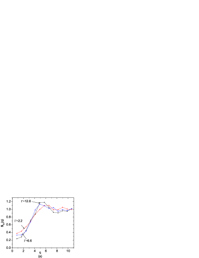
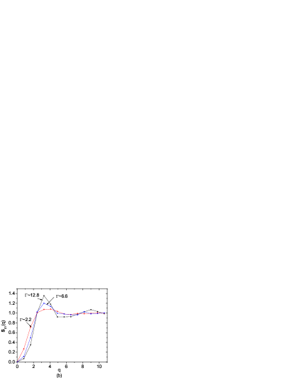
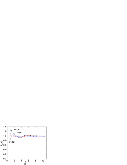
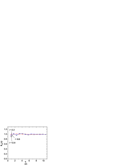
Figure 1: ${\bf S}_{0l}(q)$ from SU(2) Molecular Dynamics.

The remaining 3 hydrodynamical modes $L,E,N$ are more involved as they mix in (VI.11) and under general symmetry consideration. Indeed current conservation, ties the L mode to the N mode for instance. Most of the symmetry arguments regarding the generic nature of $\Omega_{l}$ in baus carry to our case for each color representation. Thus, for the 3 remaining non-transverse modes (VI.11) reads in matrix form

$$\left(\begin{array}[]{ccc}{\bf G}_{lNN}&{\bf G}_{lNL}&{\bf G}_{lNE}\\ {\bf G}_{lLN}&{\bf G}_{lLL}&{\bf G}_{lLE}\\ {\bf G}_{lEN}&{\bf G}_{lEL}&{\bf G}_{lEE}\end{array}\right)=\left(\begin{array}[]{ccc}z&-\Omega_{lNL}&0\\ -\Omega_{lLN}&z-\Omega_{lLL}&-\Omega_{lLE}\\ 0&-\Omega_{lEL}&z-\Omega_{lEE}\end{array}\right)^{-1}\left(\begin{array}[]{ccc}1+n\,{\bf h}_{l}&0&0\\ 0&1&0\\ 0&0&1\end{array}\right)$$ (VII.4)

The 3 remaining hydrodynamical modes are the zeros of the determinant

$$\Delta_{l}=\left|\begin{array}[]{ccc}z&-\Omega_{lNL}(zk)&0\\ -\Omega_{lLN}(zk)&z-\Omega_{lLL}(zk)&-\Omega_{lLE}(zk)\\ 0&-\Omega_{lEL}(zk)&z-\Omega_{lEE}(zk)\end{array}\right|=0$$ (VII.5)

(VII.5) admits infinitly many solutions $z_{l}(k)$. We seek the hydrodynamical solutions as analytical solutions in $k$ for small $k$, ie. $z(k)=\sum_{n}z_{ln}k^{n}$ for each SU(2) color representation $l$. In leading order, we have

$$\Delta_{l}\approx z_{l0}\left(z_{l0}^{2}-\frac{k^{2}T}{m}\,{\bf S}_{0l}^{-1}(k\approx 0)\right)\approx 0$$ (VII.6)

after using the symmetry properties of $\Omega_{l}$ as in baus for each $l$. We have also made use of the generalized Ornstein-Zernicke equations for each $l$ representation cho&zahed3 In Fig. 1 we show the molecular dynamics simulation results for 4 typical structure factors cho&zahed3

$${\bf S}_{0l}(\boldsymbol{k})=\left({\frac{4\pi}{2l+1}}\right)\left<\left|\sum_{jm}\,e^{{i\boldsymbol{k}}\cdot{\boldsymbol{x}_{j}(0)}}\,Y_{l}^{m}(\boldsymbol{Q}_{i})\,\right|^{2}\right>$$ (VII.7)

for $l=0,1,2,3$. We have made use of the dimensionless wavenumber $q=k\,a_{WS}$ with $a_{WS}$ is the Wigner-size radius. In Fig. 2 we show the analytical result for ${\bf S}_{01}$ which we will use for the numerical estimates below. We note that the $l=1$ structure factor which amounts to the monopole structure factor vanishes at $k=0$. All other $l$’s are finite at $k=0$ with $l=0$ corresponding to the density structure factor.

(VII.6) displays 3 hydrodynamical zeros as $k\rightarrow 0$ for each $l$ representation. One is massless and we identify it with the diffusive heat mode. The molecular dynamics simulations of the structure factors in Fig. 1 implies that all $l\neq 0$ channels are sound dominated with two massless modes, while the $l=1$ is plasmon dominated with two massive longitudinal plasmon states. Thus

$$z_{l\pm}=\pm\omega_{p}^{2}\delta_{l1}$$ (VII.8)

with $\omega_{p}=k_{D}\sqrt{T/m}$ the plasmon frequency. The relevance of this channel to the energy loss has been discussed in cho&zahed5 . We used ${\bf S}_{01}(k\approx 0)\approx k^{2}/k_{D}^{2}$ with $k_{D}^{2}$ the squared Debye momentum. All even $l\neq 1$ are contaminated by the sound modes. The SU(2) classical and colored Coulomb plasma supports plasmon oscillations even at strong coupling. These modes are important in the attenuation of soft monopole color oscilations.

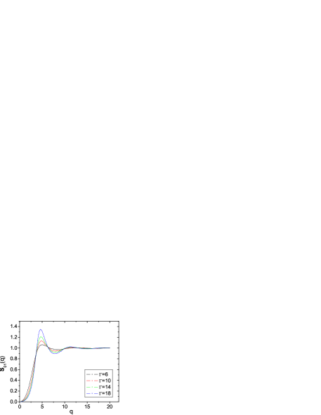
Figure 2: ${\bf S}_{01}(q)$ for different $\Gamma$ cho&zahed3

.

VIII Shear Viscosity

The transport parameters associated to the SU(2) classical and colored Coulomb plasma follows from the hydrodynamical projection and expansion discussed above. This includes, the heat diffusion coefficient, the transverse shear viscosity and the longitudinal plasmon frequency and damping parameters. In this section, we discuss explicitly the shear viscosity coefficient for the SU(2) colored Coulomb plasma.

Throughout, we define $\lambda=\frac{4}{3}\pi(3\Gamma)^{3/2}$, the bare Coulomb interaction $\bar{V}_{l}=k_{0}^{2}/l^{2}$ in units of the Wigner-size radius $k^{-1}_{0}=a_{WS}$. While varying the Coulomb coupling

$$\Gamma=\frac{g^{2}}{4\pi}\beta\frac{C_{2}}{a_{WS}}$$ (VIII.1)

all length scales will be measured in $a_{WS}=(4\pi n/3)^{-1/3}$, all times in the inverse plasmon frequency $1/\omega_{p}$ with $\omega_{p}^{2}={\kappa_{D}^{2}}/{m\beta}={n}g^{2}C_{2}/m$. All units of mass will be measured in $m$. The Debye momentum is $\kappa_{D}^{2}=g^{2}n\beta C_{2}$ and the plasma density is $n$. for instance, the shear viscosity will be expressed in fixed dimensionless units of $\eta_{*}=nm\omega_{p}a_{WS}^{2}$.

The transverse shear viscosity follows from (VII.1) with $\Sigma_{l}$ contributing to the direct or hydrodynamical part, and $\Theta_{l}$ contributing to the indirect or single-particle part. For $l=0$

$$\frac{\eta_{0}}{\eta^{*}}=\frac{\eta_{0\,dir}}{\eta^{*}}+\frac{\eta_{0\,ind}}{\eta^{*}}$$ (VIII.2)

respectively. The direct or hydrodynamical contribution is likely to be dominant at strong coupling, while the indirect or single-particle contribution is likely to take over at weak coupling. We now proceed to show that.

The indirect contribution to the viscosity follows from the contribution outside the hydrodynamical subspace through ${\cal Q}_{H}$ and lumps the single-particle phase contributions. It involves the inversion of ${\cal Q}_{H}\Sigma_{C0}{\cal Q}_{H}$ in (B.13) with

$$\eta_{0\rm ind}=\lim_{k\to 0}\frac{mn}{k^{2}}\frac{|\langle t|\Sigma_{0}|tl\rangle|^{2}}{\langle tl|i\Sigma_{0}|tl\rangle}=\lim_{k\to 0}\frac{mn}{k^{2}}\frac{|\langle t|(\Sigma_{00}+\Sigma_{C0})|tl\rangle|^{2}}{\langle tl|i\Sigma_{C0}|tl\rangle}$$ (VIII.3)

In short we expand $\Sigma_{C0}$ in terms of generalized Hermite polynomials, with the first term identified with the stress tensor due to the projection operator (D.3). The inversion follows by means of the first Sonine polynomial expansion. Explicitly

$$\eta_{ind}=\frac{\eta_{0\,ind}}{\eta_{*}}=nm\lim_{k\to 0}\frac{1}{k^{2}}\frac{|\langle t|\Sigma_{00}+\Sigma_{C0}(\boldsymbol{k},0)|lt\rangle|^{2}}{\langle lt|i\Sigma_{C0}(\boldsymbol{k},0)|lt\rangle}=\frac{(1+\lambda I_{2})^{2}}{\lambda I_{3}}$$ (VIII.4)

with

$$I_{2}=\frac{1}{60\pi^{2}}\frac{1}{(3\Gamma)^{1/2}}\int_{0}^{\infty}dq\Big{(}2({\bf S}_{01}(q)^{2}-1)+(1-{\bf S}_{01}(q))\Big{)}$$

$$I_{3}=\frac{1}{10\pi^{3/2}}\frac{1}{3\Gamma}\int_{0}^{\infty}dqq(1-{\bf S}_{01}(q))$$ (VIII.5)

with the dimensionless wave number $q=ka_{WS}$.

We recall that ${\bf S}_{01}$ is the monopole structure factor discussed in cho&zahed3 both analytically and numerically. In Fig. 2 we show the behavior of the static monopole structure factor from cho&zahed3 for different Coulomb couplings. The larger $\Gamma$ the stronger the first peak, and the oscillations. These features characterize the onset of the crystalline structure in the SU(2) colored Coulomb plasma. A good fit to Fig. 2 follows from the following parametrization

$$1+C_{0}e^{-q/C_{1}}\sin{((q-C_{2})/C_{3})}$$ (VIII.6)

with 4 parameters $C_{0,1,2,3}$. The fit following from (VIII.6) extends to $q\approx 100$ within $10^{-5}$ accuracy, thanks to the exponent.

The direct contribution to the shear viscosity follows from similar arguments. From (VII.1) and (VII.3), we have in the zero momentum limit

$$\eta_{0\,dir}=\lim_{k\to 0}\frac{mn}{k^{2}}\langle t|i\Sigma_{0}|t\rangle=\lim_{k\to 0}\frac{mn}{k^{2}}\langle t|i\Sigma_{C0}(0,0)|t\rangle$$ (VIII.7)

with $\Sigma_{0}=\Sigma_{00}+\Sigma_{I0}+\Sigma_{C0}$ as defined in (VI.3) and (V.9). Only those nonvanishing contributions after the hydrodynamical projection were retained in the second equalities in (VIII.3) as we detail in Appendix D. A rerun of the arguments yields

$$\eta_{dir}^{*} = \eta_{0\,dir}/\eta_{*}=\lambda\frac{\omega_{p}}{\kappa_{D}^{3}}\lim_{k\to 0}\frac{1}{\boldsymbol{k}^{2}}\int\frac{d\boldsymbol{l}}{(2\pi)^{3}}\int_{0}^{\infty}dtn(\boldsymbol{\epsilon}\cdot\boldsymbol{l})^{2}$$

$$\times \bigg{(}{\bf c}_{D1}(l){\cal G}_{n1}(\boldsymbol{k}-\boldsymbol{l},t){\cal G}_{n1}(\boldsymbol{l},t)\bar{V}_{\boldsymbol{l}}-{\bf c}_{D0}(l){\cal G}_{n1}(\boldsymbol{k}-\boldsymbol{l},t){\cal G}_{n1}(\boldsymbol{l},t)\bar{V}_{\boldsymbol{k}-\boldsymbol{l}}\bigg{)}$$

The projected non-static structure factor is

$${\cal G}_{n1}(\boldsymbol{l},t) = \frac{1}{n}\int d\boldsymbol{p}d\boldsymbol{p}^{\prime}\,{\bf S}_{1}(\boldsymbol{l},t;\boldsymbol{p}\boldsymbol{p}^{\prime})={\overline{\cal G}}_{n1}(\boldsymbol{l},t)\,{\bf S}_{01}(\boldsymbol{l})$$ (VIII.9)

with the normalization ${\overline{\cal G}}_{n1}(\boldsymbol{l},0)=1$. As in the one component Coulomb plasma studied in gould&mazenko we will approximate the dynamical part by its intermediate time-behavior where the motion is free. This consists in solving (IV.1) with no self-energy kernel or $\Sigma=0$,

$${\cal G}_{n1}(\boldsymbol{l},t)\approx e^{-(lt)^{2}/2m\beta}\,{\bf S}_{01}(\boldsymbol{l})$$ (VIII.10)

Thus inserting (VIII.10) and performing the integrations with $k\rightarrow 0$ yield the direct contribution to the shear viscosity

$$\eta_{dir}^{*}=\frac{\eta_{dir}}{\eta_{0}}=\frac{\sqrt{3}}{45\pi^{1/2}}\Gamma^{\frac{1}{2}}$$ (VIII.11)

The full shear viscosity result is then

$$\frac{\eta_{0}}{\eta^{*}}=\frac{\eta_{0\,dir}}{\eta^{*}}+\frac{\eta_{0\,ind}}{\eta^{*}}=\frac{\sqrt{3}}{45\pi^{1/2}}\Gamma^{\frac{1}{2}}+\frac{(1+\lambda I_{2})^{2}}{\lambda I_{3}}$$ (VIII.12)

after inserting (VIII.4) and (VIII.11) in (VIII.2). The result (VIII.12) for the shear viscosity of the transverse sound mode is analogous to the result for the sound velocity in the one component plasma derived initially in wallenborn&baus with two differences: 1/ The SU(2) Casimir in $\Gamma$; 2/ the occurrence of ${\bf S}_{01}$ instead of ${\bf S}_{00}$. Since ${\bf S}_{01}$ is plasmon dominated at low momentum, we conclude that the shear viscosity is dominated by rescattering against the SU(2) plasmon modes in the cQGP.

Using the fitted monopole structure factor (VIII.6) in (VIII.5) we can numerically assess (VIII.4) for different values of $\Gamma$. Combining this result for the indirect viscosity together with (VIII.11) for the direct viscosity yield the colorless or sound viscosity $\eta_{0}$. The values of $\eta_{0}$ are displayed in Table I, and shown in Fig. 3 (black). The SU(2) molecular dynamics simulations in gelmanetal which are parameterized as

$$\eta^{*}_{MD}\simeq 0.001\Gamma+\frac{0.242}{\Gamma^{0.3}}+\frac{0.072}{\Gamma^{2}}$$ (VIII.13)

are also displayed in Table I and shown in Fig. 3 (red) for comparison. The sound viscosity dips at about $\Gamma\approx 8$ in our analytical estimate. To understand the origin of the minimum, we display in Fig. 4 the scaling with $\Gamma$ of the direct or hydrodynamical and the indirect part of the shear viscosity. The direct contribution to the viscosity grows like $\Gamma^{1/2}$, the indirect contribution drops like $1/\Gamma^{5/2}$. The latter dominates at weak coupling, while the former dominates at strong coupling. This is indeed expected, since the direct part is the contribution from the hydrodynamical part of the phase space, while the indirect part is the contribution from the non-hydrodynamical or single-particle part of phase space. The crossing is at $\Gamma\approx 4$.

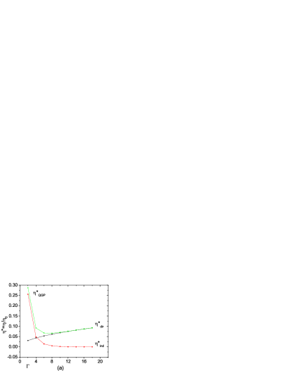
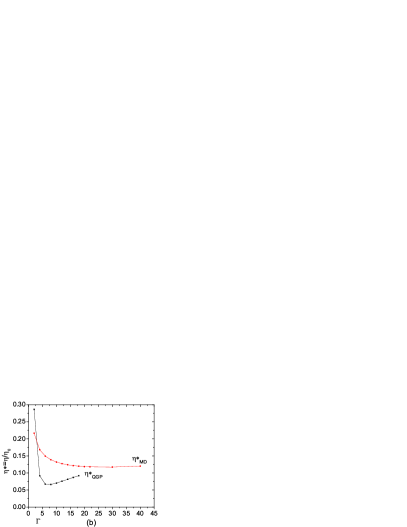
Figure 3: The direct and indirect part of the viscosity

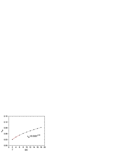
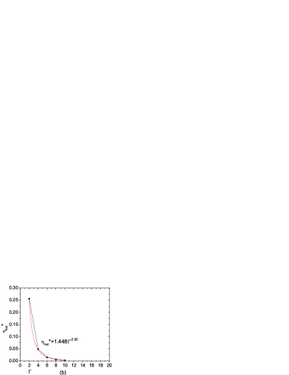
Figure 4: The best fit of the direct and indirect part of the viscosity

Table 1: Reduced shear viscosity. See text.

$\Gamma$	$2$	$4$	$6$	$8$	$10$	$12$	$14$	$16$	$18$
$\eta^{*}_{QGP}$	$0.286$	$0.092$	$0.067$	$0.066$	$0.070$	$0.076$	$0.081$	$0.087$	$0.092$
$\eta_{MD}$	$0.217$	$0.168$	$0.168$	$0.139$	$0.132$	$0.127$	$0.124$	$0.122$	$0.120$

The reduced sound velocity $\eta_{*}$ is dimensionless. To restore dimensionality and compare with expectations for an SU(2) colored Coulomb plasma, we first note that the particle density is about $3\times\,0.244\,T^{3}=0.732\,T^{3}$. There are 3 physical gluons, each carrying black-body density. The corresponding Wigner-Seitz radius is then $a_{WS}=({3}/{4\pi n})^{{1}/{3}}\approx{0.688}/{T}$. The Coulomb coupling is $\Gamma\approx 1.453\,({g^{2}N_{c}}/{4\pi})$. Since the plasmon frequency is $\omega_{p}^{2}={\kappa_{D}^{2}}/{m\beta}={n}g^{2}N_{c}/m$, we get $\omega_{p}^{2}\simeq 3.066\,T^{2}({g^{2}N_{c}}/{4\pi})$ with $m\simeq 3T$. The unit of viscosity $\eta_{0}=nm\omega_{p}a_{WS}^{2}$ translates to $1.822\,T^{3}({g^{2}}N_{c}/4\pi)^{{1}/{2}}$. In these units, the viscosity for the SU(2) cQGP dips at about $0.066$ which is $\eta^{*}_{QGP}\approx 0.066\,\eta_{0}\approx 0.120\,T^{3}\,(g^{2}N_{c}/4\pi)^{1/2}$. Since the entropy in our case is $\sigma=6\,(4\pi^{2}/90)T^{3}$, we have for the SU(2) ratio $\eta/\sigma|_{SU(2)}=0.046\,(g^{2}N_{c}/4\pi)^{1/2}$. The minimum in the viscosity occurs at $\Gamma=1.453\,({g^{2}N_{c}}/{4\pi})\approx 8$, so that $({g^{2}N_{c}}/{4\pi})^{1/2}\approx 2.347$. Thus, our shear viscosity to entropy ratio is $\eta/\sigma|_{SU(2)}\simeq 0.107$. A rerun of these estimates for SU(3) yields $\eta/\sigma|_{SU(3)}\simeq 0.078$ which is lower than the bound $\eta/\sigma=1/4\pi\simeq 0.0795$ suggested from holography.

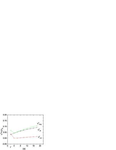
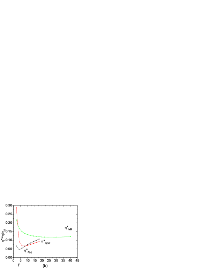
Figure 5: Comparison with weak coupling. See text.

Finally, we show in Fig. 5 the shear viscosity $\eta*_{S(q)}$ at low $\Gamma$ (a:green) and large $\Gamma$ (b:black) assessed using the weak-coupling structure factor $S(k)=k^{2}/(k^{2}+k_{D}^{2})$. The discrepancy is noticeable for $\Gamma$ near the liquid point. The large discrepancy for small values of $\Gamma$ reflects on the fact that the integrals in (VIII.5) are infrared sensitive. The sensitivity is tamed by our analytical structure factor and the simulations. We recall that in weak coupling, the Landau viscosity $\eta_{L}$ is ichimaru3

$$\frac{\eta_{L}}{\eta^{*}}=\frac{5\sqrt{3\pi}}{18}\frac{1}{\Gamma^{5/2}}\frac{1}{{\rm ln}(r_{D}/r_{0})}$$ (VIII.14)

which follows from a mean-field analysis of the kinetic equation with the plasma dielectric constant set to 1. The logarithmic dependence in (VIII.14) reflects on the infrared and ultraviolet sensitivity of the mean-field approximation. Typically $r_{D}=1/k_{D}$ and $r_{0}=(g^{2}C_{2}/4\pi)\beta$ which are the Debye length and the the distance of closest approach. Thus

$$\frac{\eta_{L}}{\eta^{*}}\approx\frac{5\sqrt{3\pi}}{27}\frac{1}{\Gamma^{5/2}}\frac{1}{{\rm ln}(1/\Gamma)}$$ (VIII.15)

or $\eta_{L}/\eta^{*}\approx 0.6/(\Gamma^{5/2}{\rm ln}(1/\Gamma))$ which is overall consistent with our analysis.

The Landau or mean-field result is smaller for the viscosity than the result from perturbative QCD. Indeed, the unscaled Landau viscosity (VIII.15) reads

$$\eta_{L}\approx\frac{10}{24}\frac{\sqrt{m}}{(\alpha_{s}C_{2})^{2}\beta^{5/2}}\frac{1}{\alpha_{s}}$$ (VIII.16)

after restoring the viscosity unit $\eta^{*}=nm\omega_{p}a_{WS}^{2}$ and using ${\rm ln}(r_{D}/r_{0})\approx 3{\rm ln}(1/\alpha_{s})/2$ with $\alpha_{s}=g^{2}/4\pi$. While our consituent gluons carry $m\approx\pi T$, in the mean field or weak coupling we can set their masses to $m\approx gT$. With this in mind, and setting $C_{2}=N_{c}=3$ in (VIII.16) we obtain

$$\eta_{L}\approx\frac{5\sqrt{2}}{108\pi^{1/4}}\frac{T^{3}}{\alpha_{s}^{7/4}{\rm ln}(1/\alpha_{s})}\approx 0.05\frac{T^{3}}{\alpha_{s}^{7/4}{\rm ln}(1/\alpha_{s})}$$ (VIII.17)

which is to be compared with the QCD weak coupling result heiselberg

$$\eta_{QCD}\approx\frac{T^{3}}{\alpha_{s}^{2}{\rm ln}(1/\alpha_{s})}$$ (VIII.18)

The mean-field result (VIII.17) is $\alpha_{s}^{1/4}\approx\sqrt{g}$ smaller in weak coupling than the QCD perturbative result. The reason is the fact that in perturbative QCD the viscosity is not only caused by collisions with the underlying parton constituents, but also quantum recombinations and decays. These latter effects are absent in our classical QGP.

IX Diffusion Constant

The calculation of the diffusion constant in the SU(2) plasma is similar to that of the shear viscosity. The governing equation is again (III.7) with $\Sigma$ and ${\bf S}$ replaced by $\Sigma_{s}$, ${\bf S}_{s}$. The label is short for single particle. The difference between ${\bf S}$ and ${\bf S}_{s}$ is the substitution of (II.7) by

$$f_{s}(\boldsymbol{r}\boldsymbol{p}\boldsymbol{Q}t)=\sqrt{N}\delta(\boldsymbol{r}-\boldsymbol{r}_{1}(t))\delta(\boldsymbol{p}-\boldsymbol{p}_{1}(t))\delta(\boldsymbol{Q}-\boldsymbol{Q}_{1}(t))$$ (IX.1)

The diffusion constant follows from the velocity auto-correlator

$$V_{D}(t)=\frac{1}{3}\langle\boldsymbol{V}(t)\cdot\boldsymbol{V}(0)\rangle$$ (IX.2)

through

$$D=\int_{0}^{\infty}dtV_{D}(t)$$ (IX.3)

Solving (III.7) using the method of one-Sonine polynomial approximation as in gould&mazenko yields the Langevin-like equation

$$\frac{dV_{D}(t)}{dt}=-\int_{0}^{t}dt^{\prime}M(t^{\prime})V_{D}(t-t^{\prime})$$ (IX.4)

with the memory kernel tied to $\Sigma_{C0}^{S}$,

$$n\,f_{0}(\boldsymbol{p}^{\prime})\,\Sigma_{Cl}^{S}(t,\boldsymbol{k},\boldsymbol{p}\boldsymbol{p}^{\prime})$$

$$=-\frac{1}{\beta}\int d\boldsymbol{p}_{1}d\boldsymbol{p}_{2}\int\frac{d\boldsymbol{l}}{(2\pi)^{3}}\boldsymbol{l}\cdot\nabla_{\boldsymbol{p}}\boldsymbol{l}\cdot\nabla_{\boldsymbol{p}^{\prime}}{\bf c}_{D1}(l)V_{\boldsymbol{l}}$$

$$\times\Big{(}\frac{l}{2l+1}{\bf S}_{l-1}^{S}(t,\boldsymbol{k}-\boldsymbol{l},\boldsymbol{p}\boldsymbol{p}^{\prime}){\bf S}_{1}(t,\boldsymbol{l},\boldsymbol{p}_{1}\boldsymbol{p}_{2})+\frac{l+1}{2l+1}{\bf S}_{l+1}^{S}(t,\boldsymbol{k}-\boldsymbol{l},\boldsymbol{p}\boldsymbol{p}^{\prime}){\bf S}_{1}(t,\boldsymbol{l},\boldsymbol{p}_{1}\boldsymbol{p}_{2})\Big{)}$$

(IX.5)

and

$$n\,f_{0}(\boldsymbol{p}^{\prime})\,\Sigma_{C0}^{S}(t,\boldsymbol{k}=\boldsymbol{0},\boldsymbol{p}\boldsymbol{p}^{\prime})$$

$$=-\frac{1}{\beta}\int d\boldsymbol{p}_{1}d\boldsymbol{p}_{2}\int\frac{d\boldsymbol{l}}{(2\pi)^{3}}\boldsymbol{l}\cdot\nabla_{\boldsymbol{p}}\boldsymbol{l}\cdot\nabla_{\boldsymbol{p}^{\prime}}{\bf c}_{D1}(l)V_{\boldsymbol{l}}{\bf S}_{1}^{S}(t,\boldsymbol{l},\boldsymbol{p}\boldsymbol{p}^{\prime}){\bf S}_{1}(t,\boldsymbol{l},\boldsymbol{p}_{1}\boldsymbol{p}_{2})$$ (IX.6)

therefore

$$M(t)=\frac{\beta}{3m}\int d\boldsymbol{p}d\boldsymbol{p}^{\prime}\boldsymbol{p}\cdot\boldsymbol{p}^{\prime}\Sigma_{C0}^{S}(t,\boldsymbol{k}=\boldsymbol{0},\boldsymbol{p}\boldsymbol{p}^{\prime})f_{0}(\boldsymbol{p}^{\prime})$$ (IX.7)

which clearly projects out the singlet color contribution. If we introduce the dimensionless diffusion constant, $D^{*}=D/w_{p}a_{WS}^{2}$, then (IX.3) together with (IX.4) yield

$$\frac{1}{D}=m\beta\int_{0}^{\infty}dtM(t)\rightarrow\frac{1}{D^{*}}=3\Gamma\int_{0}^{\infty}w_{p}dt\frac{M(t)}{w_{p}^{2}}=3\Gamma\int_{0}^{\infty}d\tau\bar{M}(\tau)$$ (IX.8)

Using similar steps as for the derivation of the viscosity, we can unwind the self-energy kernel $\Sigma_{s}$ in (IX.8) to give

$$\frac{1}{D^{*}}=-\Gamma\int\frac{d\boldsymbol{l}}{(2\pi)^{3}}\int_{0}^{\infty}d\tau\boldsymbol{l}^{2}{\bf c}_{D1}(l)V_{\boldsymbol{l}}{\cal G}_{n1}^{S}(l,t)\,{\cal G}_{n1}(l,t)$$ (IX.9)

where we have used the same the half-renormalization method discussed above for the viscosity. The color integrations are done by Legendre transforms. Here again, we separate the time-dependent structure factors as ${\cal G}_{n1}(l,t)={\bf S}_{01}(l)\bar{\cal G}_{n1}(l,t)$ and ${\bf S}_{01}^{S}(l,t)=\bar{\cal G}_{n1}(l,t)$ in the free particle approximation. Thus

$$\frac{1}{D^{*}}=\Gamma^{3/2}\Big{(}\frac{1}{3\pi}\Big{)}^{\frac{1}{2}}\int_{0}^{\infty}dqq(1-{\bf S}_{01}(q))$$ (IX.10)

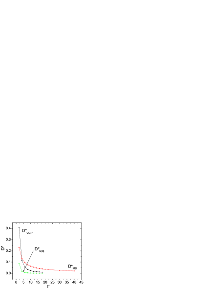
Figure 6: Diffusion Constant (black, green) versus molecular dynamics simulations (red). See text.

Table 2: Diffusion constant. See text.

$\Gamma$	$2$	$4$	$6$	$8$	$10$	$12$	$14$	$16$	$18$
$D^{*}_{QGP}$	$0.410$	$0.115$	$0.055$	$0.034$	$0.024$	$0.017$	$0.014$	$0.012$	$0.010$
$D^{*}_{MD}$	$0.230$	$0.132$	$0.095$	$0.076$	$0.063$	$0.055$	$0.048$	$0.044$	$0.040$

The results following from (IX.10) are displayed in Table LABEL:DIFF and in Fig. 6 (black) from weak to strong coupling. For comparison, we also show the the diffusion constant measured using molecular dynamics simulations with an SU(2) colored Coulomb plasma gelmanetal . The molecular dynamics simulations are fitted to

$$D^{*}\simeq\frac{0.4}{\Gamma^{0.8}}$$ (IX.11)

For comparison, we also show the diffusion constant (IX.10) assessed using the weak coupling or Debye structure factor $S(k)=k^{2}/(k^{2}+k_{D}^{2})$ in Fig. 6 (green). The discrepancy between the analytical results at small $\Gamma$ are similar to the ones we noted above for the shear viscosity. In our correctly resummed structure factor of Fig. 2, the infrared behavior of the cQGP is controlled in contrast to the simple Debye structure factor.

Finally, a comparison of (IX.10) to (VIII.5) shows that $1/D^{*}\approx 1/\lambda I_{3}$ which is seen to grow like $\Gamma^{3/2}$. Thus $D^{*}$ drops like $1/\Gamma^{3/2}$ which is close to the numerically generated result fitted in Fig. 7 (left). The weak coupling self-diffusion coefficient scales as $1/\Gamma^{5/2}$ as shown in Fig. 7 (right). More importantly, the diffusion constant in the SU(2) colored Coulomb plasma is caused solely by the non hydrodynamical modes or single particle collisions in our analysis. It does not survive at strong coupling where most of the losses are caused by the collective sound and/or plasmon modes. This result is in contrast with the shear viscosity we discussed above, where the hydrodynamical modes level it off at large $\Gamma$.

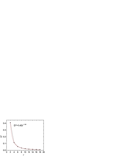
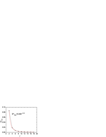
Figure 7: Fit to the diffusion constant. See text.

X Conclusions

We have provided a general framework for discussing non-perturbative many-body dynamics in the colored SU(2) Coulomb plasma introduced in SZ_newqgp . The framework extends the analysis developed intially for one-component Abelian plasmas to the non-Abelian case. In the latter, the Liouville operator is supplemented by a color precessing contribution that contributes to the connected part of the self-energy kernel.

The many-body content of the SU(2) colored Coulomb plasma are best captured by the Liouville equation in phase space in the form of an eigenvalue-like equation. Standard projected perturbation theory like analysis around the static phase space distributions yield a resummed self energy kernel in closed form. Translational space invariance and rigid color rotational invariance in phase space simplifies the nature of the kernel.

In the hydrodynamical limit, the phase space projected equations for the time-dependent and resummed structure factor displays both transverse and longitudinal hydrodynamical modes. The shear viscosity and longitudinal diffusion constant are expressed explicitly in terms of the resummed self-energy kernel. The latter is directly tied with the interacting part of the Liouville operator in color space. We have shown that in the free streaming approximation and half-renormalized Liouville operators, the transport parameters are finite.

We have explicitly derived the shear viscosity and longitudinal diffusion constant of the SU(2) colored Coulomb plasma in terms of the monopole static structure factor and the for all values of the classical Coulomb parameter $\Gamma=V/K$, the ratio of the potential to kinetic energy per particle. The results compare fairly with molecular dynamics simulations for SU(2).

The longitudinal diffusion constant is found to drop from weak to strong coupling like $1/\Gamma^{3/2}$. The shear viscosity is found to reach a minimum for $\Gamma$ of about 8. The large increase at weak coupling is the result of the large mean free paths and encoded in the direct or driving part of the connected self-energy. The minimum at intermediate $\Gamma$ is tied with the onset of hydrodynamics which reflects on the liquid nature of the colored Coulomb plasma in this regime.

At larger values of $\Gamma$ an SU(2) crystal forms as reported in SZ_newqgp . Our current analysis should be able to account for the emergence of elasticities, with in particular an elastic shear mode. This point will be pursued in a future investigation. The many body analysis presented in this work treats the color degrees of freedom as massive constituents with a finite mass and a classical SU(2) color charge. The dynamical analysis is fully non-classical. In a way, quantum mechanics is assumed to generate the constituent degrees of freedom with their assigned parameters. While this picture is supported by perturbation theory at very weak coupling, its justification at strong coupling is by no means established.

Appendix A SU(2) color phase space

A useful parametrization of the SU(2) color phase space is through the canonical variables $Q^{1},\pi^{1}$ johnson ; litim&manuel

$$Q^{1}=\cos\phi_{1}\sqrt{J^{2}-\pi_{1}^{2}},\quad Q^{2}=\sin\phi_{1}\sqrt{J^{2}-\pi_{1}^{2}},\quad Q^{3}=\pi^{1}$$ (A.1)

with $Q^{2}$ being a constraint variable fixed by $J^{2}$ or the quadratic Casimir with $q_{2}=\sum_{\alpha}^{N_{c}^{2}-1}{Q^{\alpha}Q^{\alpha}}$. The conjugate set $Q^{1},\pi^{1}$ obeys standard Poisson bracket. The associated phase space measure is

$$dQ=c_{R}d\pi_{1}d\phi_{1}JdJ\delta(J^{2}-q_{2})$$ (A.2)

where $c_{R}$ is a representation dependent constant. A simpler parametrization of the phase space is to use

$$dQ=\sin{\theta}d\theta d\phi$$ (A.3)

with the normalizations $\int dQ=4\pi$, $\sum_{\alpha}Q^{\alpha}Q^{\alpha}=1$ and $\int dQ\boldsymbol{Q}\cdot\boldsymbol{Q}=4\pi$. The SU(2) Casimir is then restored by inspection.

Appendix B Projection Method

If we define the phase space density, $\delta f_{l}^{m}(\boldsymbol{k}\boldsymbol{p},t)$

$$\delta f_{l}^{m}(\boldsymbol{k}\boldsymbol{p},t)=\sum_{i=1}^{N}e^{-i\boldsymbol{k}\cdot\boldsymbol{r}_{i}(t)}\delta(\boldsymbol{p}-\boldsymbol{p}_{i}(t)){Y_{l}^{m}}(\boldsymbol{Q}_{i})-nf_{0}(\boldsymbol{p})\delta_{l0}\delta_{m0}\delta_{\boldsymbol{k}\boldsymbol{0}}Y_{0}^{0}$$ (B.1)

we can construct structure factor ${\bf S}_{l}(t,\boldsymbol{k},\boldsymbol{p}\boldsymbol{p}^{\prime})$ for $l$th partial wave

$$\frac{4\pi}{2l+1}\sum_{m}(\delta{f_{l}^{m}}^{*}(\boldsymbol{k}\boldsymbol{p},t)|\delta f_{l}^{m}(\boldsymbol{k}\boldsymbol{p}^{\prime},0))$$

$$\equiv\frac{4\pi}{2l+1}\sum_{m}\sum_{i,j}^{N}(e^{-i\boldsymbol{k}\cdot(\boldsymbol{r}_{i}(t)-\boldsymbol{r}_{j}(t))}\delta(\boldsymbol{p}-\boldsymbol{p}_{i}(t))\delta(\boldsymbol{p}^{\prime}-\boldsymbol{p}_{j}){Y_{l}^{m}}^{*}(\boldsymbol{Q}_{i}){Y_{l}^{m}}(\boldsymbol{Q}_{j}))-n^{2}f_{0}(\boldsymbol{p})f_{0}(\boldsymbol{p}^{\prime})$$

$$\equiv{\bf S}_{l}(t,\boldsymbol{k},\boldsymbol{p}\boldsymbol{p}^{\prime})$$ (B.2)

Here a scalar product $(A|B)$ is defined as $\langle A^{*}B\rangle_{eq}$. We follow mori ; akcasu&duderstadt ; baus and recast the formal Liouville equation (III.4) in the form of a formal eigenvalue-like equation in phase space

$${\bf S}_{l}(\boldsymbol{k}z;\boldsymbol{p}\boldsymbol{p}^{\prime})=(\delta{f_{l}^{m}}^{*}(\boldsymbol{k}\boldsymbol{p})|(z-\mathcal{L})^{-1}|\delta f_{l}^{m}(\boldsymbol{k}^{\prime}\boldsymbol{p}^{\prime}))$$ (B.3)

The color charge effect by partial waves is represented as $l,m$ in Eq. (B.3). If we introduce the projection operator

$$\mathcal{P}=4\pi\sum_{l,m,\boldsymbol{k}}\int d\boldsymbol{p}_{1}d\boldsymbol{p}_{2}|\delta f_{l}^{m}(\boldsymbol{k},\boldsymbol{p}_{1})\rangle{\bf S}_{0l}^{-1}(\boldsymbol{k},\boldsymbol{p}_{1},\boldsymbol{p}_{2})\langle\delta{f_{l}^{m}}^{*}(\boldsymbol{k},\boldsymbol{p}_{2})|=1-\mathcal{Q}$$ (B.4)

we can check that this projection operator satisfies $\mathcal{P}^{2}=\mathcal{P}$

$$\mathcal{P}^{2} = 4\pi\sum_{l,m,\boldsymbol{k}}\sum_{l^{\prime},m^{\prime},\boldsymbol{k}^{\prime}}\int d\boldsymbol{p}_{1}d\boldsymbol{p}_{2}d\boldsymbol{p}_{1}^{\prime}d\boldsymbol{p}_{2}^{\prime}|\delta f_{l}^{m}(\boldsymbol{k},\boldsymbol{p}_{1})){\bf S}_{0l}^{-1}(\boldsymbol{k},\boldsymbol{p}_{1},\boldsymbol{p}_{2})$$ (B.5)

$$\times 4\pi(\delta{f_{l}^{m}}^{*}(\boldsymbol{k},\boldsymbol{p}_{2})|\delta{f_{l^{\prime}}^{m^{\prime}}}(\boldsymbol{k},\boldsymbol{p}_{1}^{\prime})){\bf S}_{0l}^{-1}(\boldsymbol{k},\boldsymbol{p_{1}}^{\prime},\boldsymbol{p_{2}}^{\prime})(\delta{f_{l^{\prime}}^{m^{\prime}}}^{*}(\boldsymbol{k},\boldsymbol{p_{2}}^{\prime})|=\mathcal{P}$$

because of the translational invariance in space and the rotational invariance in color space,

$$4\pi(\delta{f_{l}^{m}}^{*}(\boldsymbol{k},\boldsymbol{p}_{2})|\delta{f_{l^{\prime}}^{m^{\prime}}}(\boldsymbol{k},\boldsymbol{p}_{1}^{\prime}))\equiv\delta_{\boldsymbol{k}\boldsymbol{k}^{\prime}}\delta_{ll^{\prime}}\delta_{mm^{\prime}}{\bf S}_{0l}(\boldsymbol{k},\boldsymbol{p}_{2},\boldsymbol{p_{1}}^{\prime})$$ (B.6)

The off-diagonal elemenets vanish in the equilibrium averaging due to phase incoherence. Therefore, the projection operator in Eq. (B.5) satisfies also $\mathcal{Q}^{2}=\mathcal{Q}$ and $\mathcal{P}\mathcal{Q}=\mathcal{Q}\mathcal{P}=0$. If we define $|F_{l}^{m}(\boldsymbol{k}\boldsymbol{p};z))$ as $|F_{l}^{m}(\boldsymbol{k}\boldsymbol{p};z))=(z-\mathcal{L})^{-1}|\delta f_{l}^{m}(\boldsymbol{k}\boldsymbol{p}))$ from Eq. (B.3), we have

$$\mathcal{P}(z-\mathcal{L})|F_{l}^{m}(\boldsymbol{k}\boldsymbol{p};z))=\mathcal{P}|\delta f_{l}^{m}(\boldsymbol{k}\boldsymbol{p}))$$ (B.7)

$\mathcal{P}$ in Eq. (B.5) is the operator which projects phase space function of a multipartle state with $l^{\prime}$th partial wave into a single particle state of the same parial wave, $|\delta f_{l^{\prime}}^{m^{\prime}}(\boldsymbol{k}\boldsymbol{p}))$, $\mathcal{P}|g_{l^{\prime}}^{m^{\prime}}(\boldsymbol{k}\boldsymbol{p}))=|\delta f_{l^{\prime}}^{m^{\prime}}(\boldsymbol{k}\boldsymbol{p}))$. Therefore $\mathcal{Q}|\delta f_{l}^{m}(\boldsymbol{k}\boldsymbol{p}))=(1-\mathcal{P})|\delta f_{l}^{m}(\boldsymbol{k}\boldsymbol{p}))=0$. With these in mind, we can modify the above equation further using $\mathcal{P}+\mathcal{Q}=I$

$$(\mathcal{P}z-\mathcal{P}\mathcal{L}\mathcal{P}-\mathcal{P}\mathcal{L}\mathcal{Q})|F_{l}^{m}(\boldsymbol{k}\boldsymbol{p};z))=\mathcal{P}|\delta f_{l}^{m}(\boldsymbol{k}\boldsymbol{p}))$$

$$(\mathcal{Q}z-\mathcal{Q}\mathcal{L}\mathcal{P}-\mathcal{Q}\mathcal{L}\mathcal{Q})|F_{l}^{m}(\boldsymbol{k}\boldsymbol{p};z))=0$$ (B.8)

From these equations, we can extract

$$z\mathcal{P}|F_{l}^{m}(\boldsymbol{k}\boldsymbol{p};z))-\mathcal{P}\mathcal{L}\mathcal{P}|F_{l}^{m}(\boldsymbol{k}\boldsymbol{p};z))-\mathcal{P}\mathcal{L}\mathcal{Q}(z-\mathcal{Q}\mathcal{L}\mathcal{Q})^{-1}\mathcal{Q}\mathcal{L}\mathcal{P}|F_{l}^{m}(\boldsymbol{k}\boldsymbol{p};z))=\mathcal{P}|\delta f_{l}^{m}(\boldsymbol{k}\boldsymbol{p}))$$ (B.9)

By multiplying $(\delta f(\boldsymbol{k}\boldsymbol{p})|$ we finally obtain,

$$z{\bf S}_{l}(\boldsymbol{k}z;\boldsymbol{p}\boldsymbol{p}^{\prime})-\int d\boldsymbol{p}_{1}d\Sigma_{l}(\boldsymbol{k}z;\boldsymbol{p}\boldsymbol{p}_{1}){\bf S}_{l}(\boldsymbol{k}z;\boldsymbol{p}_{1}\boldsymbol{p}^{\prime})={\bf S}_{l}(\boldsymbol{k}0;\boldsymbol{p}\boldsymbol{p}^{\prime})$$ (B.10)

where the memory function, or the evolution operator $\Sigma_{l}(\boldsymbol{k}z;\boldsymbol{p}\boldsymbol{p}_{1})$ is

$$\Sigma_{l}(\boldsymbol{k}z;\boldsymbol{p}\boldsymbol{p}^{\prime})=\frac{4\pi}{2l+1}\sum_{m}\int d\boldsymbol{p}_{1}(\delta{f_{l}^{m}}^{*}(\boldsymbol{k},\boldsymbol{p})|\mathcal{L}+{\Psi}|\delta f_{l}^{m}(\boldsymbol{k},\boldsymbol{p}_{1})){\bf S}_{0l}^{-1}(\boldsymbol{k},\boldsymbol{p}_{1},\boldsymbol{p}^{\prime})$$ (B.11)

with

$${\Psi}=\mathcal{P}\mathcal{L}\mathcal{Q}(z-\mathcal{Q}\mathcal{L}\mathcal{Q})^{-1}\mathcal{Q}\mathcal{L}\mathcal{P}$$ (B.12)

Since the Liouville operator $\mathcal{L}$ can be split into $\mathcal{L}_{0}+\mathcal{L}_{I}+\mathcal{L}_{Q}$, Eq. (II.9), the evolution operator can also be split into four terms; the free streaming term($\Sigma^{0}_{l}$), the self consistent term($\Sigma^{s}_{l}$), the color charge term($\Sigma^{Q}$) and the non-local collision term($\Sigma^{c}$).

$$\Sigma_{0l}(\boldsymbol{k}z;\boldsymbol{p}\boldsymbol{p}^{\prime})=\frac{\boldsymbol{k}\cdot\boldsymbol{p}}{m}\delta(\boldsymbol{p}-\boldsymbol{p}^{\prime})$$

$$\Sigma_{Il}(\boldsymbol{k}z;\boldsymbol{p}\boldsymbol{p}^{\prime})=-n\frac{\boldsymbol{k}\cdot\boldsymbol{p}}{m}f_{0}(\boldsymbol{p}){\bf c}_{Dl}(\boldsymbol{k})$$

$$\Sigma_{Ql}(\boldsymbol{k}z;\boldsymbol{p}\boldsymbol{p}^{\prime})=0$$

$$\Sigma_{Cl}(\boldsymbol{k}z;\boldsymbol{p}\boldsymbol{p}^{\prime})=\frac{1}{nf_{0}(\boldsymbol{p})}\frac{4\pi}{2l+1}\sum_{m}(\delta{f_{l}^{m}}^{*}(\boldsymbol{k}\boldsymbol{p})|\mathcal{L}\mathcal{Q}(z-\mathcal{Q}\mathcal{L}\mathcal{Q})^{-1}\mathcal{Q}\mathcal{L}|\delta f_{l}^{m}(\boldsymbol{k}\boldsymbol{p}^{\prime}))$$ (B.13)

Appendix C Collisional Color Contribution

In this Appendix we detail the calculation that leads to a zero contribution from the colored Liouville operator in the collisional part of the self energy in the free streaming approximation. A typical contribution to (V.2) and (V.5) is

$$L_{Q}(\boldsymbol{q},\boldsymbol{q}_{1})\,L^{R}_{Q}(\boldsymbol{q}^{\prime},\boldsymbol{q}_{2})\,{\bf S}(t,\boldsymbol{q},\boldsymbol{q}_{2})\,{\bf S}(t,\boldsymbol{q}^{\prime},\boldsymbol{q}_{1})=\frac{1}{\beta}$$

$$\times\bigg{(}V(\boldsymbol{r}-\boldsymbol{r}_{1})\,\boldsymbol{Q}\times\boldsymbol{Q}_{1}\cdot(\boldsymbol{\nabla}_{Q}-\boldsymbol{\nabla}_{Q_{1}})\bigg{)}$$

$$\times\bigg{(}{\bf c}^{\prime}_{D}(\boldsymbol{r}^{\prime}-\boldsymbol{r}_{2},\boldsymbol{Q}^{\prime}\cdot\boldsymbol{Q}_{2}))\,\boldsymbol{Q}^{\prime}\times\boldsymbol{Q}_{2}\cdot(\boldsymbol{\nabla}_{Q^{\prime}}-\boldsymbol{\nabla}_{Q_{2}})\bigg{)}\,\,{\bf S}(t,\boldsymbol{q},\boldsymbol{q}_{2})\,{\bf S}(t,\boldsymbol{q}^{\prime},\boldsymbol{q}_{1})$$ (C.1)

which can be reduced to

$$L_{Q}(\boldsymbol{q},\boldsymbol{q}_{1})\,L^{R}_{Q}(\boldsymbol{q}^{\prime},\boldsymbol{q}_{2})\,{\bf S}(t,\boldsymbol{q},\boldsymbol{q}_{2})\,{\bf S}(t,\boldsymbol{q}^{\prime},\boldsymbol{q}_{1})=-\frac{1}{\beta}\,V(\boldsymbol{r}-\boldsymbol{r}_{1})\,{\bf c}^{\prime}_{D}(\boldsymbol{r}^{\prime}-\boldsymbol{r}_{2},\boldsymbol{Q}^{\prime}\cdot\boldsymbol{Q}_{2}))\,$$

$$\times\Bigg{(}{\bf S}^{\prime}(\boldsymbol{Q}\cdot\boldsymbol{Q}_{2}){\bf S}^{\prime}(\boldsymbol{Q}^{\prime}\cdot\boldsymbol{Q}_{1})(\boldsymbol{Q}_{1}\times\boldsymbol{Q}_{2})\cdot\boldsymbol{Q}\,(\boldsymbol{Q}_{1}\times\boldsymbol{Q}_{2})\cdot\boldsymbol{Q}^{\prime}$$

$$\,\,\,\,\,\times{\bf S}^{\prime\prime}(\boldsymbol{Q}\cdot\boldsymbol{Q}_{2}){\bf S}(\boldsymbol{Q}^{\prime}\cdot\boldsymbol{Q}_{1})(\boldsymbol{Q}_{1}\times\boldsymbol{Q}_{2})\cdot\boldsymbol{Q}\,(\boldsymbol{Q}\times\boldsymbol{Q}^{\prime})\cdot\boldsymbol{Q}_{2}$$

$$\,\,\,\,\,\times{\bf S}(\boldsymbol{Q}\cdot\boldsymbol{Q}_{2}){\bf S}^{\prime\prime}(\boldsymbol{Q}^{\prime}\cdot\boldsymbol{Q}_{1})(\boldsymbol{Q}\times\boldsymbol{Q}^{\prime})\cdot\boldsymbol{Q}_{1}\,(\boldsymbol{Q}_{1}\times\boldsymbol{Q}_{2})\cdot\boldsymbol{Q}^{\prime}$$

$$\,\,\,\,\,\times{\bf S}^{\prime}(\boldsymbol{Q}\cdot\boldsymbol{Q}_{2}){\bf S}^{\prime}(\boldsymbol{Q}^{\prime}\cdot\boldsymbol{Q}_{1})(\boldsymbol{Q}\times\boldsymbol{Q}^{\prime})\cdot\boldsymbol{Q}_{1}\,(\boldsymbol{Q}\times\boldsymbol{Q}^{\prime})\cdot\boldsymbol{Q}_{2}\Bigg{)}$$ (C.2)

The derivatives on ${\bf c}_{D}$ and ${\bf S}$ are on their color argument. We note that (C.2) contribute to the collisional part of the self energy in (B.6) after the integration over $Q_{1}$ and $Q_{2}$, which is then zero. This is expected. Indeed, the colored Liouville operator is a 3-body force that requires 3 distinct color charges to not vanish. While (C.2) contributer to the unintegrated collisional operator, it does not in the integrated one which is the self-energy on the 2point function. It does contribute in the Liouville hierarchy in the 3-body structure factors and higher.

Appendix D Hydrodynamical subspace

The projection method onto the hydrodynamical subspace has been discussed by many foster&martin ; foster ; baus . This consists in dialing the projector in (VI.2) onto the hydrodynamical modes. We choose Hermite polynomials as a basis set with the Maxwell-Boltzman distribution $f_{0}(\boldsymbol{p})$ as a Gaussian weight function. The Hermite polynomials are the the generalized ones in 3D grad . Specifically

$$H_{1(n)}(\boldsymbol{p})=1\quad\quad H_{2(l)}(\boldsymbol{p})=p_{z}\quad\quad H_{3(\epsilon)}(\boldsymbol{p})=\frac{1}{\sqrt{6}}(p^{2}-3)$$

$$H_{4(t_{1})}(\boldsymbol{p})=p_{x}\quad\quad H_{5(t_{2})}(\boldsymbol{p})=p_{y}$$ (D.1)

These polynomials are orthonormal for the inner product

$$\langle m|n\rangle=\int d\boldsymbol{p}a_{m}H_{m}(\boldsymbol{p})a_{n}H_{n}(\boldsymbol{p})nf_{0}(\boldsymbol{p})=\delta_{mn}$$

$$\langle m|F(k,t)|n\rangle=\int d\boldsymbol{p}d\boldsymbol{p}^{\prime}a_{m}H_{m}(\boldsymbol{p})F(k,t;\boldsymbol{p}\boldsymbol{p}^{\prime})a_{n}H_{n}(\boldsymbol{p}^{\prime})nf_{0}(\boldsymbol{p}^{\prime})$$ (D.2)

Here $a_{m}$ and $a_{n}$ set the normalizations. We chose the longitudinal momentum direction along $\boldsymbol{k}$ in Fourier space, $\langle l|=a_{m}\hat{k}\cdot\boldsymbol{p}$. The transverse directional is chosen orthogonal to ${\boldsymbol{k}}$, $\langle t|=a_{m}^{\prime}\boldsymbol{\epsilon}\cdot\boldsymbol{p}$ with a unit vector satisfying $\boldsymbol{\epsilon}^{2}=1$ and $\boldsymbol{\epsilon}\cdot\hat{k}=0$.

The hydrodynamical projection operators $\mathcal{P}_{H}$ restricted to the five states (D.1) are

$$\mathcal{P}_{H}=\sum_{i}^{5}|i\rangle\langle i|\quad\quad\mathcal{Q}_{H}=1-\mathcal{P}_{H}=1-\sum_{i}^{5}|i\rangle\langle i|$$ (D.3)

While in general these 5 statesare enough to characterize the hydrodynamical modes in the SU(2) phase space, we need additional states to work out the shear viscosity as it involves in general correlations in the stress tensor through the Kubo relation hansen&mcdonald . For that we need additionally,

$$H_{6}(\boldsymbol{p})=p_{x}p_{y}\quad\quad H_{7}(\boldsymbol{p})=p_{x}p_{z}\quad\quad H_{8}(\boldsymbol{p})=p_{y}p_{z}$$ (D.4)

With the definition of $G_{ij}(\boldsymbol{k}z)=\langle i|{\bf S}(\boldsymbol{k}z;\boldsymbol{p}\boldsymbol{p}^{\prime})(nf_{0}(\boldsymbol{p}))^{-1}|j\rangle$ we can rewrite (VI.2) as

$$\Big{(}z-\sum_{k}\langle i|\Omega(\boldsymbol{k}z;\boldsymbol{p}\boldsymbol{p}^{\prime})|k\rangle\Big{)}G_{kj}(\boldsymbol{k}z)=G_{ij}(\boldsymbol{k}0)$$ (D.5)

where $i,j$ are short for: $n$(density), $\epsilon$(energy), $l$(longitudinal momentum) and $t$(transverse momentum).

References

(1)
E. V. Shuryak and I. Zahed,
Phys. Rev. C 70, 021901 (2004)
E. V. Shuryak and I. Zahed,
Phys. Rev. D 70, 054507 (2004)
(2)
D. Teaney, J. Lauret and E. V. Shuryak, Phys. Rev. Lett. 86, 4783 (2001)
D. Teaney, J. Lauret and E. V. Shuryak, nucl-th/0110037 P. F. Kolb, P.Huovinen, U. Heinz, H. Heiselberg,
Phys. Lett. B500 (2001) 232.
P. F. Kolb and U. Heinz, nucl-th/0305084
(3) B. A. Gelman, E. V. Shuryak and I. Zahed, Phys. Rev. C 74, 044908 (2006)
(4) S. Cho and I. Zahed, Phys. Rev. C 79 044911 (2009)
(5) S. Cho and I. Zahed, Phys. Rev. C 80 014906 (2009)
(6) K. Dusling and I. Zahed, arXiv:0904.0169
(7) B. A. Gelman, E. V. Shuryak and I. Zahed, Phys. Rev. C 74, 044909 (2006)
(8) S. K. Wong, Nuovo Cimento A 65, 689 (1970)
(9) S. Cho and I. Zahed, arXiv:0909.4725
(10) D. Foster and P. C. Martin, Phys. Rev. A 2, 1575 (1970)
(11) D. Foster, Phys. Rev. A 9, 943 (1974)
(12) G. F. Mazenko, Phys. Rev. A. 7, 209 (1973)
(13) G. F. Mazenko, Phys. Rev. A. 9, 360 (1974)
(14) J. Wallenborn and M. Baus, Phys. Rev, A 18, 1737 (1978)
(15) M. Baus, Physica A 79, 377 (1975)
(16) S. Cho and I. Zahed, arXiv:0910.1548
(17) H. Gould and G. F. Mazenko, Phys. Rev. A 15, 1274 (1977)