Overlapping stochastic block models with application to the French political blogosphere

Abstract

Complex systems in nature and in society are often represented as networks, describing the rich set of interactions between objects of interest. Many deterministic and probabilistic clustering methods have been developed to analyze such structures. Given a network, almost all of them partition the vertices into disjoint clusters, according to their connection profile. However, recent studies have shown that these techniques were too restrictive and that most of the existing networks contained overlapping clusters. To tackle this issue, we present in this paper the Overlapping Stochastic Block Model. Our approach allows the vertices to belong to multiple clusters, and, to some extent, generalizes the well-known Stochastic Block Model [Nowicki and Snijders (2001)]. We show that the model is generically identifiable within classes of equivalence and we propose an approximate inference procedure, based on global and local variational techniques. Using toy data sets as well as the French Political Blogosphere network and the transcriptional network of Saccharomyces cerevisiae, we compare our work with other approaches.

T1Supported in part by the French Agence Nationale de la Recherche under Grant NeMo ANR-08-BLAN-0304-01.

Overlapping stochastic block models with application to the French political blogosphere

, and

1 Introduction

Networks have been extensively studied ever since the work of Moreno (1934). They are used in many scientific fields to represent the interactions between objects of interest. For instance, in Biology, regulatory networks can describe the regulation of genes with transcriptional factors [Milo et al. (2002)], while metabolic networks focus on representing pathways of biochemical reactions [Lacroix, Fernandes and Sagot (2006)]. In the social sciences, networks are commonly used to represent relational ties between actors [Snijders and Nowicki (1997); Nowicki and Snijders (2001)].

In this context, many deterministic and probabilistic clustering methods have been used to acquire knowledge from the network topology. As shown in Newman and Leicht (2007), most of these techniques seek specific structures in networks. Thus, some models look for community structure where vertices are partitioned into classes such that vertices of a class are mostly connected to vertices of the same class [Hofman and Wiggins (2008)]. They are particularly suitable for the analysis of affiliation networks [Latouche, Birmelé and Ambroise (2009)]. Most existing community discovery algorithms are based on the modularity score of Girvan and Newman (2002). However, Bickel and Chen (2009) showed that these algorithms were (asymptotically) biased and that using modularity scores could lead to the discovery of an incorrect community structure, even for large graphs. The model of Handcock, Raftery and Tantrum (2007) which extends Hoff, Raftery and Handcock (2002) is an alternative approach. Vertices are clustered depending on their positions in a continuous latent space. They proposed a Bayesian inference procedure, based on Markov Chain Monte Carlo (MCMC), which is implemented in the R package latentnet [Krivitsky and Handcock (2009)], as well an asymptotic BIC criterion. Other models look for disassortative mixing in which vertices mostly connect to vertices of different classes. They are commonly used to analyze bipartite networks [Estrada and Rodriguez-Velazquez (2005)] which are present in many applications. For more details, see Newman and Leicht (2007).

The Stochastic Block Model (SBM) can uncover heterogeneous structures in a large variety of networks [Latouche, Birmelé and Ambroise (2009)]. Originally developed in the social sciences, SBM is a probabilistic generalization [Fienberg and Wasserman (1981); Holland, Laskey and Leinhardt (1983)] of the method described in White, Boorman and Breiger (1976). Given a network, it assumes that each vertex belongs to a latent class among $Q$ classes and uses a $Q\times Q$ connectivity matrix $\bolds{\Pi}$ to describe the connection probabilities [Frank and Harary (1982)]. No assumption is made on $\bolds{\Pi}$ such that SBM is a very flexible model. In particular, it can be used, among others, to look for community structure and disassortative mixing. Many inference methods have been employed to estimate the SBM parameters. They all face the same problem. Indeed, contrary to Gaussian mixture models or other usual mixture models, the posterior distribution $p(\mathbf{Z}|\mathbf{X})$, of all the hidden label variables, given the observation $\mathbf{X}$, cannot be factorized due to conditional dependency. Nowicki and Snijders (2001) proposed a Bayesian probabilistic approach. Their algorithm is implemented in the software BLOCKS, which is part of the package StoCNET [Boer et al. (2006)]. It uses Gibbs sampling to approximate the posterior distributions and leads to accurate a posteriori estimates. Two model based criteria have been proposed to choose the optimal value of $Q$. Thus, Daudin, Picard and Robin (2008) used an ICL criterion, based on a Laplace approximation of the Integrated Classification Likelihood, while Latouche, Birmelé and Ambroise (2009) used a nonasymptotic approximation of the marginal likelihood. For an extensive discussion on statistical network models and blockmodel selection, we refer to Goldenberg et al. (2010).

A drawback of existing graph clustering techniques is that they all partition the vertices into disjoint clusters, while lots of objects in real world applications typically belong to multiple groups or communities. For instance, many proteins, so-called moonlighting proteins, are known to have several functions in the cells [Jeffery (1999)], and actors might belong to several groups of interests [Palla et al. (2005)]. Thus, a graph clustering method should be able to uncover overlapping clusters. This issue has received growing attention in the last few years, starting with an algorithmic approach based on small complete sub-graphs developed by Palla et al. (2005) and implemented in the software CFinder [Palla et al. (2006)]. They defined a $k$-clique community as a union of all $k$-cliques (complete sub-graphs of size $k$) that can be reached from each other through a series of adjacent $k$-cliques. Given a network, their algorithm first locates all cliques and then identifies the communities using a clique–clique overlap matrix [Everett and Borgatti (1998)]. By construction, the resulting communities can overlap. In order to select the optimal value of $k$, the authors suggested a global criterion which looks for a community structure as highly connected as possible. Small values of $k$ lead to a giant community which smears the details of a network by merging small communities. Conversely, when $k$ increases, the communities tend to become smaller, more disintegrated, but also more cohesive. Therefore, they proposed a heuristic which consists in running their algorithm for various values of $k$ and then to select the lowest value such that no giant community appears.

More recent work [Airoldi et al. (2008)] proposed the Mixed Membership Stochastic Block model (MMSB) which has been used with success to analyze networks in many applications [Airoldi et al. (2007); Airoldi et al. (2006)]. They used variational techniques to estimate the model parameters and proposed a criterion to select the number of classes. As detailed in Heller, Williamson and Ghahramani (2008), mixed membership models, as Latent Dirichlet Allocation [Blei, Ng and Jordan (2003)], are flexible models which can capture partial membership [Griffiths and Ghahramani (2005); Heller and Ghahramani (2007)], in the form of attribute-specific mixtures. In MMSB, a mixing weight vector $\bolds{\pi}_{i}$ is drawn from a Dirichlet distribution for each vertex in the network, $\pi_{iq}$ being the probability of vertex $i$ to belong to class $q$. The edge probability from vertex $i$ to vertex $j$ is then given by $p_{ij}=\mathbf{Z}_{i\rightarrow j}^{\top}\mathbf{B}\mathbf{Z}_{i\leftarrow i}$, where $\mathbf{B}$ is a $Q\times Q$ matrix of connection probabilities similar to the $\bolds{\Pi}$ matrix in SBM. The vector $\mathbf{Z}_{i\rightarrow j}$ is sampled from a multinomial distribution $\mathcal{M}(1,\bolds{\pi}_{i})$ and describes the class membership of vertex $i$ in its relation toward vertex $j$. By symmetry, the vector $\mathbf{Z}_{i\leftarrow j}$ is drawn from a multinomial distribution $\mathcal{M}(1,\bolds{\pi}_{j})$ and represents the class membership of vertex $j$ in its relation toward vertex $i$. Thus, depending on its relations with other vertices, each vertex can belong to different classes and, therefore, MMSB can be viewed as allowing overlapping clusters. However, the limit of MMSB is that it does not produce edges which are themselves influenced by the fact that some vertices belong to multiple clusters. Indeed, for every pair $(i,j)$ of vertices, only a single draw of $\mathbf{Z}_{i\rightarrow j}$ and $\mathbf{Z}_{i\leftarrow j}$ determines the probability $p_{ij}$ of an edge, all the other class memberships of vertex $i$ and $j$ toward other vertices in the network do not play a part. In this paper we present a complementary approach which tackles this issue.

Fu and Banerjee (2008) modeled overlapping clusters on $Q$ components by characterizing each individual $i$ by a latent $\{0,1\}$ vector $z_{i}$ of length $Q$ drawn from independent Bernoulli distributions. The $i$th row of the data matrix then only depends on $z_{i}$. In the underlying clustering structure, $i$ belongs to the components corresponding to a $1$ in $z_{i}$. Nevertheless, the proposed model needs $Q$ parameters for each individual and supposes independence between rows and columns of the data matrix, which is not the case when looking for network structures.

In this paper we propose a new model for generating networks, depending on $(Q+1)^{2}+Q$ parameters, where $Q$ is the number of components in the mixture. A latent $\{0,1\}$-vector of length $Q$ is assigned to each vertex, drawn from products of Bernoulli distributions whose parameters are not vertex-dependent. Each vertex may then belong to several components, allowing overlapping clusters, and each edge probability depends only on the components of its endpoints.

In Section 2 we briefly review the stochastic block model introduced by Nowicki and Snijders (2001). In Section 3 we present the overlapping stochastic block model and we show in Section 4 that the model is identifiable within classes of equivalence. In Section 5 we propose an EM-like algorithm to infer the parameters of the model. Finally, in Section 6 we compare our work with other approaches using simulated data and two real networks. We show the efficiency of our model to detect overlapping clusters in networks.

2 The stochastic block model

In this paper we consider a directed binary random graph $\mathcal{G}$ represented by an $N\times N$ binary adjacency matrix $\mathbf{X}$. Each entry $X_{ij}$ describes the presence or absence of an edge from vertex $i$ to vertex $j$. We assume that $\mathcal{G}$ does not have any self loop, and, therefore, the variables $X_{ii}$ will not be taken into account. The Stochastic Block Model (SBM) introduced by Nowicki and Snijders (2001) associates to each vertex of a network a latent variable $\mathbf{Z}_{i}$ drawn from a multinomial distribution:

$$\mathbf{Z}_{i}\sim\mathcal{M}\bigl{(}1,\bolds{\alpha}=(\alpha_{1},\alpha_{2},\dots,\alpha_{Q})\bigr{)},$$

where $\bolds{\alpha}$ denotes the vector of class proportions. As in other standard mixture models, the vector $\mathbf{Z}_{i}$ sees all its components set to zero except one such that $Z_{iq}=1$ if vertex $i$ belongs to class $q$. The model then verifies

$$\sum_{q=1}^{Q}Z_{iq}=1\qquad\forall i\in\{1,\dots,N\}$$ (1)

and

$$\sum_{q=1}^{Q}\alpha_{q}=1.$$ (2)

Finally, the edges of the network are drawn from a Bernoulli distribution:

$$X_{ij}|\{Z_{iq}Z_{jl}=1\}\sim\mathcal{B}(\pi_{ql}),$$

where $\bolds{\Pi}$ is a $Q\times Q$ matrix of connection probabilities. According to this model, the latent variables $\mathbf{Z}_{1},\dots,\mathbf{Z}_{N}$ are i.i.d. and given this latent structure, all the edges are supposed to be independent. Note that SBM was originally described in a more general setting, allowing any discrete relational data. However, as explained previously, we concentrate in the following on binary edges only.

3 The overlapping stochastic block model

In order to allow each vertex to belong to multiple classes, we relax the constraints (1) and (2). Thus, for each vertex $i$ of the network, we introduce a latent vector $\mathbf{Z}_{i}$, of $Q$ independent Boolean variables $Z_{iq}\in\{0,1\}$, drawn from a multivariate Bernoulli distribution:

$$\mathbf{Z}_{i}\sim\prod_{q=1}^{Q}\mathcal{B}(Z_{iq};\alpha_{q})=\prod_{q=1}^{Q}\alpha_{q}^{Z_{iq}}(1-\alpha_{q})^{1-Z_{iq}}.$$ (3)

We point out that $\mathbf{Z}_{i}$ can also have all its components set to zero which is a useful feature in practice as described in Sections 3.2 and 6. The edge probabilities are then given by

$$X_{ij}|\mathbf{Z}_{i},\mathbf{Z}_{j}\sim\mathcal{B}(X_{ij};\mathrm{g}(a_{\mathbf{Z}_{i},\mathbf{Z}_{j}}))=e^{X_{ij}a_{\mathbf{Z}_{i},\mathbf{Z}_{j}}}\mathrm{g}(-a_{\mathbf{Z}_{i},\mathbf{Z}_{j}}),$$

where

$$a_{\mathbf{Z}_{i},\mathbf{Z}_{j}}=\mathbf{Z}^{\top}_{i}\mathbf{W}\mathbf{Z}_{j}+\mathbf{Z}_{i}^{\top}\mathbf{U}+\mathbf{V}^{\top}\mathbf{Z}_{j}+W^{*},$$ (4)

and $\mathrm{g}(x)=(1+e^{-x})^{-1}$ is the logistic sigmoid function. $\mathbf{W}$ is a $Q\times Q$ real matrix, whereas $\mathbf{U}$ and $\mathbf{V}$ are $Q$-dimensional real vectors. The first term in the right-hand side of (4) describes the interactions between the vertices $i$ and $j$. If $i$ belongs only to class $q$ and $j$ only to class $l$, then only one interaction term remains ($\mathbf{Z}_{i}^{\top}\mathbf{W}\mathbf{Z}_{j}=W_{ql}$). However, as illustrated in Table 1, the model can take more complex interactions into account if one or both of these two vertices belong to multiple classes (Figure 1). Note that the second term in (4) does not depend on $\mathbf{Z}_{j}$. It models the overall capacity of vertex $i$ to connect to other vertices. By symmetry, the third term represents the global tendency of vertex $j$ to receive an edge. These two parameters $\mathbf{U}$ and $\mathbf{V}$ are related to the sender/receiver effects $\delta_{i}$ and $\gamma_{j}$ in the Latent Cluster Random Effects Model (LCREM) of Krivitsky et al. (2009). However, contrary to LCREM, $\delta_{i}=\mathbf{Z}_{i}^{\top}\mathbf{U}$ and $\gamma_{j}=\mathbf{V}^{\top}\mathbf{Z}_{j}$ depend on the classes. In other words, two different vertices sharing the same classes will have exactly the same sender/receiver effects, which is not the case in LCREM. Finally, we use the scalar $W^{*}$ as a bias, to model sparsity.

Table 1: The values of $a_{\mathbf{Z}_{i},\mathbf{Z}_{j}}$ in functions of $\mathbf{Z}_{i}$ (rows) and $\mathbf{Z}_{j}$ (columns) for an overlapping stochastic block model with $Q=2$

	$\bolds{(0,0)}$	$\bolds{(1,0)}$	$\bolds{(0,1)}$	$\bolds{(1,1)}$
$(0,0)$	$W^{*}$	$V_{1}+W^{*}$	$V_{2}+W^{*}$	$V_{1}+V_{2}+W^{*}$
$(1,0)$	$U_{1}+W^{*}$	$W_{11}+U_{1}+V_{1}+W^{*}$	$W_{12}+U_{1}+V_{2}+W^{*}$	$W_{11}+W_{12}+U_{1}$
				${}+V_{1}+V_{2}+W^{*}$
$(0,1)$	$U_{2}+W^{*}$	$W_{21}+U_{2}+V_{1}+W^{*}$	$W_{22}+U_{2}+V_{2}+W^{*}$	$W_{21}+W_{22}+U_{2}$
				${}+V_{1}+V_{2}+W^{*}$
$(1,1)$	$U_{1}+U_{2}+W^{*}$	$W_{11}+W_{21}+U_{1}$	$W_{12}+W_{22}+U_{1}$	$W_{11}+W_{12}+W_{21}$
		${}+U_{2}+V_{1}+W^{*}$	${}+U_{2}+V_{2}+W^{*}$	${}+W_{22}+U_{1}+U_{2}$
				${}+V_{1}+V_{2}+W^{*}$

Figure 1: Example of a directed graph with three overlapping clusters.

If we associate to each latent variable $\mathbf{Z}_{i}$ a vector $\widetilde{\mathbf{Z}}_{i}=(\mathbf{Z}_{i},1)^{\top}$, then (4) can be written

$$a_{\mathbf{Z}_{i},\mathbf{Z}_{j}}=\widetilde{\mathbf{Z}}{}_{i}^{\top}\widetilde{\mathbf{W}}\widetilde{\mathbf{Z}}_{j},$$ (5)

where

$$\widetilde{\mathbf{W}}=\pmatrix{\mathbf{W}&\mathbf{U}\cr\mathbf{V}^{\top}&W^{*}}.$$

The $\widetilde{Z}_{i(Q+1)}$’s can be seen as random variables drawn from a Bernoulli distribution with probability $\alpha_{Q+1}=1$. Thus, one way to think about the model is to consider that all the vertices in the graph belong to a $(Q+1)$th cluster which is overlapped by all the other clusters. In the following, we will use (5) to simplify the notation.

Finally, given the latent structure $\mathbf{Z}=\{\mathbf{Z}_{1},\dots,\mathbf{Z}_{N}\}$, all the edges are supposed to be independent (see Figure 2). Thus, when considering directed graphs without self-loop, the Overlapping Stochastic Block Model (OSBM) is defined through the following distributions:

$$p(\mathbf{Z}|\bolds{\alpha})=\prod_{i=1}^{N}\prod_{q=1}^{Q}\alpha_{q}^{Z_{iq}}(1-\alpha_{q})^{1-Z_{iq}}$$ (6)

and

$$p(\mathbf{X}|\mathbf{Z},\widetilde{\mathbf{W}})=\prod_{i\neq j}^{N}e^{X_{ij}a_{\mathbf{Z}_{i},\mathbf{Z}_{j}}}{g}(-a_{\mathbf{Z}_{i},\mathbf{Z}_{j}}).$$

Figure 2: Graphical representation of the overlapping stochastic block model.

3.1 Modeling sparsity

As explained in Airoldi et al. (2008), real networks are often sparse and it is crucial to distinguish the two sources of noninteraction. Sparsity might be the result of the rarity of interactions in general, but it might also indicate that some class (intra or inter) connection probabilities are close to zero. For instance, social networks (see Section 6.2) are often made of communities where vertices are mostly connected to vertices of the same community. This corresponds to classes with high intra connection probabilities and low inter connection probabilities. In (4) we can notice that $W^{*}$ appears in $a_{\mathbf{Z}_{i},\mathbf{Z}_{j}}$ for every pair of vertices. Therefore, $W^{*}$ is a convenient parameter to model the two sources of sparsity. Indeed, low values of $W^{*}$ result from the rarity of interactions in general, whereas high values signify that sparsity comes from the classes (parameters in $\mathbf{W}$, $\mathbf{U}$ and $\mathbf{V}$).

3.2 Modeling outliers

When applied on real networks, graph clustering methods often lead to giant classes of vertices having low output and input degrees [Daudin, Picard and Robin (2008); Latouche, Birmelé and Ambroise (2009)]. These classes are usually discarded and the analysis of networks focus on more highly structured classes to extract useful information. The product of Bernoulli distributions (6) provides a natural way to encode these “outliers.” Indeed, rather than using giant classes, OSBM uses the null component such that $\mathbf{Z}_{i}=\mathbf{0}$ if vertex $i$ is an outlier and should not be classified in any class.

4 Identifiability

Before looking for an optimization procedure to estimate the model parameters, given a sample of observations (a network), it is crucial to verify whether OSBM is identifiable. A theorem of Allman, Matias and Rhodes (2009) lies at the core of the results presented in this section.

If we denote $\mathcal{F}(\Theta)=\{\mathbb{P}_{\bolds{\theta}},\bolds{\theta}\in\Theta\}$, a family of models we are interested in, the classical definition of identifiability requires that for any two different values $\bolds{\theta}\neq\bolds{\theta}^{\prime}$, the corresponding probability distributions $\mathbb{P}_{\bolds{\theta}}$ and $\mathbb{P}_{\bolds{\theta}^{\prime}}$ are different.

4.1 Correspondence with (nonoverlapping) stochastic block models

Let $\Theta_{\mathrm{OSBM}}$ be the parameter space of the family of OSBMs with $Q$ classes:

$$\Theta_{\mathrm{OSBM}}=\bigl{\{}(\bolds{\alpha},\widetilde{\mathbf{W}})\in[0,1]^{Q}\times\mathbb{R}^{(Q+1)^{2}}\bigr{\}}.$$

Each $\bolds{\theta}$ in $\Theta_{\mathrm{OSBM}}$ corresponds to a random graph model which is defined by the distribution $p(\mathbf{X}|\bolds{\alpha},\widetilde{\mathbf{W}})$. The aim of this Section is to characterize whether there exists any relation between two different parameters $\bolds{\theta}$ and $\bolds{\theta}^{\prime}$ in $\Theta_{\mathrm{OSBM}}$, leading to the same random graph model.

We consider the (nonoverlapping) Stochastic Block Model (SBM) introduced by Nowicki and Snijders (2001). The model is defined by a set of classes $\mathcal{C}$, a vector of class proportions $\bolds{\gamma}=\{\gamma_{\mathbf{C}}\}_{\mathbf{C}\in\mathcal{C}}$ verifying $\sum_{\mathbf{C}\in\mathcal{C}}\gamma_{\mathbf{C}}=1$, and a matrix of connection probabilities $\bolds{\Pi}=(\Pi_{\mathbf{C},\mathbf{D}})_{\mathbf{C},\mathbf{D}\in\mathcal{C}^{2}}$. Note that they are an infinite number of ways to represent and encode the classes. For simplicity, a common choice is to set $\mathcal{C}=\{1,\dots,Q\}$ and possibly $\mathcal{C}=\{\mathbf{C}\in\{0,1\}^{Q},\sum_{q=1}^{Q}C_{q}=1\}$, for a model with $Q$ classes. The random graphs are drawn as follows. First, the class of each vertex is sampled from a multinomial distribution with parameters $(1,\bolds{\gamma})$. Thus, each vertex $i$ belongs only to one class, and that class is $\mathbf{C}$ with probability $\gamma_{\mathbf{C}}$. Second, the edges are drawn independently from each other from Bernoulli distributions, the probability of an edge $(i,j)$ being $\Pi_{\mathbf{C},\mathbf{D}}$, if $i$ belongs to class $\mathbf{C}$ and $j$ to class $\mathbf{D}$.

Let $\Theta_{\mathrm{SBM}}$ be the parameter space of the family of SBMs with $2^{Q}$ classes:

$$\Theta_{\mathrm{SBM}}=\biggl{\{}(\bolds{\gamma},\bolds{\Pi})\in[0,1]^{2^{Q}}\times[0,1]^{2^{2Q}},\sum_{\mathbf{C}\in\mathcal{C}}\gamma_{\mathbf{C}}=1\biggr{\}}.$$

Considering that each possible value of the vectors $\mathbf{Z}_{i}$’s in an OSBM with $Q$ classes encodes a class in a SBM with $2^{Q}$ classes (i.e., $\mathcal{C}=\{0,1\}^{Q}$) yields a natural function:

$$\phi\dvtx\begin{array}[]{rcl}\Theta_{\mathrm{OSBM}}&\rightarrow&\Theta_{\mathrm{SBM}}\\ (\bolds{\alpha},\widetilde{\mathbf{W}})&\rightarrow&(\bolds{\gamma},\bolds{\Pi})\end{array},$$

where

$$\gamma_{\mathbf{C}}=\prod_{q=1}^{Q}\alpha_{q}^{C_{q}}(1-\alpha_{q})^{1-C_{q}}\qquad\forall\mathbf{C}\in\{0,1\}^{Q},$$

and

$$\Pi_{\mathbf{C},\mathbf{D}}=g(\mathbf{C}^{\top}\mathbf{W}\mathbf{D}+\mathbf{C}^{\top}\mathbf{U}+\mathbf{V}^{\top}\mathbf{D}+W^{*})$$

$$\eqntext{\forall(\mathbf{C},\mathbf{D})\in\{0,1\}^{Q}\times\{0,1\}^{Q}.}$$ (7)

Let $\mathcal{G}_{N}$ denote the set of probability measures on the graphs of $N$ vertices. The OSBM of parameter $\bolds{\theta}$ in $\Theta_{\mathrm{OSBM}}$ and the SBM of parameter $\phi(\bolds{\theta})$ in $\Theta_{\mathrm{SBM}}$ clearly induce the same measure $\mu$ in $\mathcal{G}_{N}$. Thus, denoting by $\psi(\bolds{\gamma},\bolds{\Pi})$ the probability measure in $\mathcal{G}_{N}$ induced by the SBM of parameter $(\bolds{\gamma},\bolds{\Pi})$, the problem of identifiability is to characterize the relations between parameters $\bolds{\theta}\in\Theta_{\mathrm{OSBM}}$ and $\bolds{\theta}^{\prime}\in\Theta_{\mathrm{OSBM}}$ such that $\psi(\phi(\bolds{\theta}))=\psi(\phi(\bolds{\theta}^{\prime}))$:

$$\begin{array}[]{ccccc}\Theta_{\mathrm{OSBM}}&\rightarrow&\Theta_{\mathrm{SBM}}&\rightarrow&\mathcal{G}_{N},\\ \bolds{\theta}=(\bolds{\alpha},\widetilde{\mathbf{W}})&\stackrel{{\scriptstyle\phi}}{{\rightarrow}}&(\bolds{\gamma},\bolds{\Pi})&\stackrel{{\scriptstyle\psi}}{{\rightarrow}}&\mu.\end{array}$$

The identifiability of SBM was studied by Allman, Matias and Rhodes (2009), who showed that the model is generically identifiable up to a permutation of the classes. In other words, except in a set of parameters which has a null Lebesgue measure, two parameters imply the same random graph model if and only if they differ only by the ordering of the classes. Therefore, the main theorem of Allman, Matias and Rhodes (2009) implies the following result.

Theorem 4.1

There exists a set $\Theta_{\mathrm{SBM}}^{\mathrm{bad}}\subset\Theta_{\mathrm{SBM}}$ of null Lebesgue measure such that, for every $(\bolds{\gamma},\bolds{\Pi})$ and $(\bolds{\gamma}^{\prime},\bolds{\Pi}^{\prime})$ not in $\Theta_{\mathrm{SBM}}^{\mathrm{bad}}$, $\psi(\bolds{\gamma},\bolds{\Pi})=\psi(\bolds{\gamma}^{\prime},\bolds{\Pi}^{\prime})$ if and only if there exists a function $P_{\nu}$ such that $(\bolds{\gamma}^{\prime},\bolds{\Pi}^{\prime})=P_{\nu}((\bolds{\gamma},\bolds{\Pi}))$, where:

• [$\bullet$]

• $\nu$ is a permutation on $\{0,1\}^{Q}$,

• $\bolds{\gamma}^{\prime}_{\mathbf{C}}=\bolds{\gamma}_{\nu(\mathbf{C})},\forall\mathbf{C}\in\{0,1\}^{Q}$,

• $\bolds{\Pi}^{\prime}_{\mathbf{C},\mathbf{D}}=\Pi_{\nu(\mathbf{C}),\nu(\mathbf{D})},\forall(\mathbf{C},\mathbf{D})\in\{0,1\}^{Q}\times\{0,1\}^{Q}$.

Thus, studying the generical identifiability of the OSBM is equivalent to characterizing the parameters of $\Theta_{\mathrm{OSBM}}$ verifying $\phi(\bolds{\theta}^{\prime})=P_{\nu}(\phi(\bolds{\theta}))$ for some permutation $\nu$ on $\{0,1\}^{Q}$.

4.2 Permutations and inversions

As in the case of the SBM, reordering the $Q$ classes of the OSBM and doing the corresponding modification in $\bolds{\alpha}$ and $\widetilde{\mathbf{W}}$ does not change the generative random graph model. Indeed, let $\sigma$ be a permutation on $\{1,\dots,Q\}$ and let $P_{\sigma}$ denote the function corresponding to the permutation $\sigma$ of the classes. Then, $(\bolds{\alpha}^{\prime},\widetilde{\mathbf{W}}^{\prime})=P_{\sigma}(\bolds{\alpha},\widetilde{\mathbf{W}})$ is defined by

$$\alpha_{q}^{\prime}=\alpha_{\sigma(q)}\qquad\forall q\in\{1,\dots,Q\},$$

and

$$\widetilde{\mathbf{W}}^{\prime}_{q,l}=\widetilde{\mathbf{W}}_{\sigma(q),\sigma(l)}\qquad\forall(q,l)\in\{1,\dots,Q+1\}^{2}.$$

Now, let $\nu$ be the permutation of $\{0,1\}^{Q}$ defined by

$$\nu(\mathbf{C})=\bigl{(}C_{\sigma(1)},\ldots,C_{\sigma(Q)}\bigr{)}\qquad\forall\mathbf{C}\in\{0,1\}^{Q}.$$

It is then straightforward to see that, for every parameter $\bolds{\theta}$ in $\Theta_{\mathrm{OSBM}}$ and every permutation $\sigma$, $\phi(P_{\sigma}(\bolds{\theta}))=P_{\nu}(\phi(\bolds{\theta}))$, where $P_{\nu}$ is defined in Theorem 4.1.

There is another family of operations in $\Theta_{\mathrm{OSBM}}$ which does not change the generative random graph model, which we call inversions. They correspond to exchanging the labels $0$ to $1$ and vice versa on some of the coordinates of the $Z_{i}$’s. To give an intuition, consider a parameter $\bolds{\theta}=(\bolds{\alpha},\widetilde{\mathbf{W}})$ in $\Theta_{\mathrm{OSBM}}$. Let us generate graphs under the probability measure in $\mathcal{G}_{N}$ induced by $\bolds{\theta}$ and consider only the first coordinate of the $Z_{i}$’s. If we denote by “cluster 1” the vertices whose $Z_{i}$’s have a $1$ as first coordinate, the graph sampling procedure consists in sampling the set “cluster 1” and then drawing the edges conditionally on that information. Note that it would be equivalent to sample the vertices which are not in “cluster 1” and to draw the edges conditionally on that information. Thus, there exists an equivalent reparametrization where the $1$’s in the first coordinate correspond to the vertices which are not in “cluster 1.” This is the parameter $\bolds{\theta}^{\prime}$ obtained from $\bolds{\theta}$ by an inversion of the first coordinate.

Let $\mathbf{A}$ be any vector of $\{0,1\}^{Q}$. We define the $A$-inversion $I_{\mathbf{A}}$ as follows:

$$I_{\mathbf{A}}\dvtx\begin{array}[]{rcl}\Theta_{\mathrm{OSBM}}&\rightarrow&\Theta_{\mathrm{OSBM}}\\ (\bolds{\alpha},\widetilde{\mathbf{W}})&\rightarrow&(\bolds{\alpha}^{\prime},\widetilde{\mathbf{W}}^{\prime})\end{array},$$

where

$$\alpha^{\prime}_{j}=\cases{1-\alpha_{j},&\quad\mbox{if } $A_{j}=1$,\cr\alpha_{j},&\quad\mbox{otherwise}}\qquad\forall j\in\{1,\ldots,Q\},$$

and

$$\widetilde{\mathbf{W}}^{\prime}=\mathbf{M}_{\mathbf{A}}^{\top}\widetilde{\mathbf{W}}\mathbf{M}_{\mathbf{A}}.$$

The matrix $\mathbf{M}_{\mathbf{A}}$ is defined by

$$\mathbf{M}_{\mathbf{A}}=\pmatrix{I-2\operatorname{diag}(\mathbf{A})&\mathbf{A}\cr 0\enskip\cdots\enskip 0&1},$$

with $\operatorname{diag}(\mathbf{A})$ being the $Q\times Q$ diagonal matrix whose diagonal is the vector $\mathbf{A}$.

Proposition 4.1

For every $\mathbf{A}\in\{0,1\}^{Q}$, let $\nu$ be the permutation of $\{0,1\}^{Q}$ defined by

$$\forall\mathbf{C}\in\{0,1\}^{Q}\qquad\nu(\mathbf{C})_{i}=\cases{1-C_{i},&\quad\mbox{if } $A_{i}=1$,\cr C_{i},&\quad\mbox{otherwise}.}$$

Then, for every $\bolds{\theta}$ in $\Theta_{\mathrm{OSBM}}$,

$$\phi(I_{\mathbf{A}}(\bolds{\theta}))=P_{\nu}(\phi(\bolds{\theta})),$$

where $P_{\nu}$ is defined in Theorem 4.1.

Consider $\bolds{\theta}\in\Theta_{\mathrm{OSBM}}$ and $\mathbf{A}\in\{0,1\}^{Q}$ and define $(\bolds{\gamma},\bolds{\Pi})=\phi(\bolds{\theta})$ and $(\bolds{\gamma}^{\prime},\bolds{\Pi}^{\prime})=\phi(I_{\mathbf{A}}(\bolds{\theta})).$ It is straightforward to verify that

$$\bolds{\gamma}^{\prime}_{\mathbf{C}}=\bolds{\gamma}_{\nu(\mathbf{C})}\qquad\forall\mathbf{C}\in\{0,1\}^{Q}.$$

Moreover, since $M_{\mathbf{A}}\left({\mathbf{C}\atop 1}\right)=\left({\nu(\mathbf{C})\atop 1}\right)$, it follows that

$$\bolds{\Pi}^{\prime}_{\mathbf{C},\mathbf{D}} = g\left(\pmatrix{\mathbf{C}^{\top}&1}\mathbf{M}_{\mathbf{A}}^{\top}\widetilde{\mathbf{W}}\mathbf{M}_{\mathbf{A}}\pmatrix{\mathbf{D}\cr 1}\right)$$

$$= g\left(\pmatrix{\nu(\mathbf{C})^{\top}&1}\widetilde{\mathbf{W}}\pmatrix{\nu(\mathbf{D})\cr 1}\right)$$

$$= \bolds{\Pi}_{\nu(\mathbf{C}),\nu(\mathbf{D})}.$$

Therefore, $\phi(I_{A}(\bolds{\theta}))=P_{\nu}(\phi(\bolds{\theta}))$ .

4.3 Identifiability

Let us define the following equivalence relation:

$$\bolds{\theta}\sim\bolds{\theta}^{\prime}\qquad\mbox{if }\exists\sigma,\mathbf{A}|\bolds{\theta}^{\prime}=I_{\mathbf{A}}(P_{\sigma}(\bolds{\theta})).$$

To be convinced that it is an equivalence relation, note that

$$I_{\mathbf{A}}\circ P_{\sigma}=P_{\sigma}\circ I_{\sigma^{-1}(\mathbf{A})}.$$

Consider the set of equivalence classes for the relation $\sim$. It follows that:

• Two parameters in the same equivalence class induce the same measure in $\mathcal{G}_{N}$.

• Each equivalence class contains a parameter $\bolds{\theta}=(\bolds{\alpha},\widetilde{\mathbf{W}})$ such that $\alpha_{1}\leq\alpha_{2}\leq\cdots\leq\alpha_{Q}\leq\frac{1}{2}$. Moreover, if the $\alpha_{i}$’s are all distinct and strictly lower than $\frac{1}{2}$, there is a unique such parameter in the equivalence class.

We are now able to state our main theorem about identifiability, that is, that the model is generically identifiable up to the equivalence relation $\sim$.

Theorem 4.2

For every $\bolds{\alpha}\in\,]0,1[^{Q}$, let $\beta\in\mathbb{R}^{Q}$ be the vector defined by $\beta_{k}=-\ln(\frac{\alpha_{k}}{1-\alpha_{k}})$, for every $k$.

Define $\Theta_{\mathrm{OSBM}}^{\mathrm{bad}}$ as the set of parameters $(\bolds{\alpha},\widetilde{\mathbf{W}})$ such that one of the following conditions holds:

• there exists $1\leq k\leq Q$ such that $\alpha_{k}=0$ or $\alpha_{k}=1$ or $\alpha_{k}=\frac{1}{2}$,

• there exist $1\leq k,l\leq Q$ such that $\alpha_{k}=\alpha_{l}$,

• there exist $\mathbf{C},\mathbf{D}\in\{0,1\}^{Q}\times\{0,1\}^{Q}$ such that $\sum_{k}\beta_{k}C_{k}=\sum_{k}\beta_{k}D_{k}$,

• $\phi(\bolds{\alpha},\widetilde{\mathbf{W}})\in\Theta_{\mathrm{SBM}}^{\mathrm{bad}}$, set of null measure given by Theorem 4.1.

Then $\Theta_{\mathrm{OSBM}}^{\mathrm{bad}}$ has a null Lebesgue measure on $\Theta_{\mathrm{OSBM}}$ and

$$\forall\bolds{\theta},\bolds{\theta}^{\prime}\in(\Theta_{\mathrm{OSBM}}\setminus\Theta_{\mathrm{OSBM}}^{\mathrm{bad}})^{2}\qquad\phi(\bolds{\theta})=\phi(\bolds{\theta}^{\prime})\quad\Longleftrightarrow\quad\bolds{\theta}\sim\bolds{\theta}^{\prime}.$$

$\Theta_{\mathrm{OSBM}}^{\mathrm{bad}}$ is the union of a finite number of hyperplanes or spaces which are isomorphic to hyperplanes. Therefore, $\mu(\Theta_{\mathrm{OSBM}}^{\mathrm{bad}})=0$.

Let $\bolds{\theta}=(\bolds{\alpha},\widetilde{\mathbf{W}})$, $\bolds{\theta}^{\prime}=(\bolds{\alpha}^{\prime},\widetilde{\mathbf{W}}^{\prime})$, $\phi(\bolds{\theta})=(\bolds{\gamma},\bolds{\Pi})$ and $\phi(\bolds{\theta}^{\prime})=(\bolds{\gamma}^{\prime},\bolds{\Pi}^{\prime})$. As $\phi$ is constant on each equivalence class and as $\bolds{\theta}$ and $\bolds{\theta}^{\prime}$ are not in $\Theta_{\mathrm{OSBM}}^{\mathrm{bad}}$, we can assume that $0<\alpha_{1}<\cdots<\alpha_{k}<\frac{1}{2}$ and $0<\alpha^{\prime}_{1}<\cdots<\alpha^{\prime}_{k}<\frac{1}{2}$. Proving the theorem is then equivalent to proving that $\bolds{\theta}=\bolds{\theta}^{\prime}$.

As $\phi(\bolds{\theta})=\phi(\bolds{\theta}^{\prime})$, Theorem 4.1 ensures that there exists a permutation $\nu\dvtx\{0,1\}^{Q}\to\{0,1\}^{Q}$ such that

$$\cases{\gamma^{\prime}_{\mathbf{C}}=\gamma_{\nu(\mathbf{C})}&\quad$\forall\mathbf{C}$,\cr\Pi^{\prime}_{\mathbf{C},\mathbf{D}}=\Pi_{\psi(\mathbf{C}),\psi(\mathbf{D})}&\quad$\forall\mathbf{C},\mathbf{D}$.}$$

Then, in particular,

$$\biggl{\{}\prod_{k}\alpha_{k}^{C_{k}}(1-\alpha_{k})^{1-C_{k}},\mathbf{C}\in\{0,1\}^{Q}\biggr{\}}$$

(8)

$$\qquad=\biggl{\{}\prod_{k}(\alpha^{\prime}_{k})^{C_{k}}(1-\alpha^{\prime}_{k})^{1-C_{k}},\mathbf{C}\in\{0,1\}^{Q}\biggr{\}}.$$

The minima of those two sets as well as the second lowest values are equal, that is,

$$\prod_{k}\alpha_{k}=\prod_{k}\alpha^{\prime}_{k}\quad\mbox{and}\quad\biggl{(}\prod_{k\leq Q-1}\alpha_{k}\biggr{)}(1-\alpha_{Q})=\biggl{(}\prod_{k\leq Q-1}\alpha^{\prime}_{k}\biggr{)}(1-\alpha^{\prime}_{Q}).$$

Dividing those equations term by term yields $\frac{\alpha_{Q}}{1-\alpha_{Q}}=\frac{\alpha^{\prime}_{Q}}{1-\alpha^{\prime}_{Q}}$ and finally $\alpha_{Q}=\alpha^{\prime}_{Q}$. Dividing all terms by $\alpha_{Q}^{C_{Q}}(1-\alpha_{Q})^{1-C_{Q}}$ in (4.3), by induction, it follows that

$$\bolds{\alpha}=\bolds{\alpha}^{\prime}.$$ (9)

Now, for any $\mathbf{C}\in\{0,1\}^{Q}$, the fact that $\bolds{\gamma}^{\prime}_{\mathbf{C}}=\bolds{\gamma}_{\nu(\mathbf{C})}$ can be written as

$$\prod_{k}\alpha_{k}^{C_{k}}(1-\alpha_{k})^{1-C_{k}} = \prod_{k}\alpha_{k}^{\nu(C)_{k}}(1-\alpha_{k})^{1-\nu(C)_{k}},$$

$$\sum_{k}C_{k}\ln\biggl{(}\frac{\alpha_{k}}{1-\alpha_{k}}\biggr{)}+\sum_{k}\ln(1-\alpha_{k}) = \sum_{k}\nu(C_{k})\ln\biggl{(}\frac{\alpha_{k}}{1-\alpha_{k}}\biggr{)}+\sum_{k}\ln(1-\alpha_{k}),$$

$$\sum_{k}\beta_{k}C_{k} = \sum_{k}\beta_{k}\nu(C)_{k}.$$

Since $\bolds{\theta}\notin\Theta_{\mathrm{OSBM}}^{\mathrm{bad}}$, this implies that $\nu(\mathbf{C})=\mathbf{C}$. As it is true for every $\mathbf{C}$, $\nu$ is in fact the identity function.

Therefore, for every $\mathbf{C},\mathbf{D}$, $\Pi_{\mathbf{C},\mathbf{D}}=\Pi^{\prime}_{\mathbf{C},\mathbf{D}}$, that is,

$$\sum_{q,l}w_{ql}c_{q}d_{l}+\sum_{q}u_{q}c_{q}+\sum_{l}v_{l}d_{l}+w^{*}=\sum_{q,l}w^{\prime}_{ql}c_{q}d_{l}+\sum_{q}u^{\prime}_{q}c_{q}+\sum_{l}v^{\prime}_{l}d_{l}+w^{\prime*}.$$

Applying it for $\mathbf{C}=\mathbf{D}=0$ implies $W^{*}=W^{\prime*}$.

Applying it for $\mathbf{D}=0$ and $\mathbf{C}=\bolds{\delta}_{q}$, where $\bolds{\delta}_{q}$ is the vector having a $1$ on the $q$th coordinate and $0$’s elsewhere yields $u_{q}+W^{*}=u^{\prime}_{q}+W^{\prime*}$ and, thus, $u_{q}=u^{\prime}_{q}$.

By symmetry, $\mathbf{C}=0$ and $\mathbf{D}=\delta_{l}$ implies $v_{l}=v^{\prime}_{l}$.

Finally, $\mathbf{C}=\delta_{q}$ and $\mathbf{D}=\delta_{l}$ gives $W_{ql}=W^{\prime}_{ql}$.

Thus,

$$\widetilde{\mathbf{W}}=\widetilde{\mathbf{W}}^{\prime}.$$ (10)

By equations (9) and (10), we have $\bolds{\theta}=\bolds{\theta}^{\prime}$.

5 Statistical inference

Given a network, our aim in this section is to estimate the OSBM parameters.

The log-likelihood of the observed data set is defined through the marginalization: $p(\mathbf{X}|\bolds{\alpha},\widetilde{\mathbf{W}})=\sum_{\mathbf{Z}}p(\mathbf{X},\mathbf{Z}|\bolds{\alpha},\widetilde{\mathbf{W}})$. This summation involves $2^{NQ}$ terms and quickly becomes intractable. To tackle this issue, the Expectation–Maximization (EM) algorithm has been applied on many mixture models. However, the E-step requires the calculation of the posterior distribution $p(\mathbf{Z}|\mathbf{X},\bolds{\alpha},\widetilde{\mathbf{W}})$ which cannot be factorized in the case of networks [see Daudin, Picard and Robin (2008) for more details]. In order to obtain a tractable procedure, we present some approximations based on global and local variational techniques.

5.1 The $q$-transformation

Given a distribution $q(\mathbf{Z})$, the log-likelihood of the observed data set can be decomposed using the Kullback–Leibler divergence $\mathrm{KL}(\cdot\|\cdot)$:

$$\ln p(\mathbf{X}|\bolds{\alpha},\widetilde{\mathbf{W}})=\mathcal{L}(q;\bolds{\alpha},\widetilde{\mathbf{W}})+\operatorname{KL}(q(\cdot)\|p(\cdot|\mathbf{X},\bolds{\alpha},\widetilde{\mathbf{W}})),$$ (11)

where

$$\mathcal{L}(q;\bolds{\alpha},\widetilde{\mathbf{W}})=\sum_{\mathbf{Z}}q(\mathbf{Z})\ln\biggl{\{}\frac{p(\mathbf{X},\mathbf{Z}|\bolds{\alpha},\widetilde{\mathbf{W}})}{q(\mathbf{Z})}\biggr{\}}$$ (12)

and

$$\operatorname{KL}(q(\cdot)\|p(\cdot|\mathbf{X},\bolds{\alpha},\widetilde{\mathbf{W}}))=-\sum_{\mathbf{Z}}q(\mathbf{Z})\ln\biggl{\{}\frac{p(\mathbf{Z}|\mathbf{X},\bolds{\alpha},\widetilde{\mathbf{W}})}{q(\mathbf{Z})}\biggr{\}}.$$ (13)

The maximum $\ln p(\mathbf{X}|\bolds{\alpha},\widetilde{\mathbf{W}})$ of the lower bound $\mathcal{L}$ (12) is reached when $q(\mathbf{Z})=p(\mathbf{Z}|\mathbf{X},\bolds{\alpha},\widetilde{\mathbf{W}})$. Thus, if the posterior distribution $p(\mathbf{Z}|\mathbf{X},\bolds{\alpha},\widetilde{\mathbf{W}})$ was tractable, the optimizations of $\mathcal{L}$ and $\ln p(\mathbf{X}|\bolds{\alpha},\widetilde{\mathbf{W}})$, with respect to $\bolds{\alpha}$ and $\widetilde{\mathbf{W}}$, would be equivalent. However, in the case of networks, $p(\mathbf{Z}|\mathbf{X},\bolds{\alpha},\widetilde{\mathbf{W}})$ cannot be calculated and $\mathcal{L}$ cannot be optimized over the entire space of $q(\mathbf{Z})$ distributions. Thus, we restrict our search to the class of distributions which satisfy

$$q(\mathbf{Z})=\prod_{i=1}^{N}q(\mathbf{Z}_{i}),$$ (14)

with

$$q(\mathbf{Z}_{i})=\prod_{q=1}^{Q}\mathcal{B}(Z_{iq};\tau_{iq})=\prod_{q=1}^{Q}\tau_{iq}^{Z_{iq}}(1-\tau_{iq})^{1-Z_{iq}}.$$

Each $\tau_{iq}$ is a variational parameter which corresponds to the posterior probability of node $i$ to belong to class $q$. As for the vector $\bolds{\alpha}$, the vectors $\bolds{\tau}_{i}=\{\tau_{i1},\dots,\tau_{iQ}\}$ are not constrained to lie in the $(Q-1)$-dimensional simplex.

Proposition 5.1

[Proof in Latouche, Birmelé and Ambroise (2010), Appendix A]. The lower bound of the observed data log-likelihood is given by

$$\mathcal{L}(q;\bolds{\alpha},\widetilde{\mathbf{W}}) = \sum_{i\neq j}^{N}\{X_{ij}\tilde{\bolds{\tau}}{}_{i}^{\top}\widetilde{\mathbf{W}}\tilde{\bolds{\tau}}_{j}+\mathrm{E}_{\mathbf{Z}_{i},\mathbf{Z}_{j}}[\ln\mathrm{g}(-a_{\mathbf{Z}_{i},\mathbf{Z}_{j}})]\}$$

$${}+\sum_{i=1}^{N}\sum_{q=1}^{Q}\{\tau_{iq}\ln\alpha_{q}+(1-\tau_{iq})\ln(1-\alpha_{q})\}$$

$${}-\sum_{i=1}^{N}\sum_{q=1}^{Q}\{\tau_{iq}\ln\tau_{iq}+(1-\tau_{iq})\ln(1-\tau_{iq})\}.$$

Unfortunately, since the logistic sigmoid function is nonlinear,$\mathrm{E}_{\mathbf{Z}_{i},\mathbf{Z}_{j}}[\ln\mathrm{g}(-a_{\mathbf{Z}_{i},\mathbf{Z}_{j}})]$ in (5.1) cannot be computed analytically. Thus, we need a second level of approximation to optimize the lower bound of the observed data set.

5.2 $\xi$-transformation

Proposition 5.2 ([Proof in Latouche, Birmelé and Ambroise (2010) in Appendix A])

Given a variational parameter $\xi_{ij}$, $\mathrm{E}_{\mathbf{Z}_{i},\mathbf{Z}_{j}}[\ln\mathrm{g}(-a_{\mathbf{Z}_{i},\mathbf{Z}_{j}})]$ satisfies

$$\mathrm{E}_{\mathbf{Z}_{i},\mathbf{Z}_{j}}[\ln\mathrm{g}(-a_{\mathbf{Z}_{i},\mathbf{Z}_{j}})]$$

$$\qquad\geq\ln\mathrm{g}(\xi_{ij})-\frac{(\tilde{\bolds{\tau}}{}_{i}^{\top}\widetilde{\mathbf{W}}\tilde{\bolds{\tau}}_{j}+\xi_{ij})}{2}-\lambda(\xi_{ij})\bigl{(}\mathrm{E}_{\mathbf{Z}_{i},\mathbf{Z}_{j}}[(\widetilde{\mathbf{Z}}{}_{i}^{\top}\widetilde{\mathbf{W}}\widetilde{\mathbf{Z}}_{j})^{2}]-\xi_{ij}^{2}\bigr{)}.$$

Eventually, a lower bound of the first lower bound can be computed:

$$\ln p(\mathbf{X}|\bolds{\alpha},\widetilde{\mathbf{W}})\geq\mathcal{L}(q;\bolds{\alpha},\widetilde{\mathbf{W}})\geq\mathcal{L}(q;\bolds{\alpha},\widetilde{\mathbf{W}},\bolds{\xi}),$$ (17)

where

$$\mathcal{L}(q;\bolds{\alpha},\widetilde{\mathbf{W}},\bolds{\xi}) = \sum_{i\neq j}^{N}\biggl{\{}\biggl{(}X_{ij}-\frac{1}{2}\biggr{)}\tilde{\bolds{\tau}}{}_{i}^{\top}\widetilde{\mathbf{W}}\tilde{\bolds{\tau}}_{j}+\ln\mathrm{g}(\xi_{ij})-\frac{\xi_{ij}}{2}$$

$${}\hskip 19.0pt-\lambda(\xi_{ij})\bigl{(}\operatorname{Tr}(\widetilde{\mathbf{W}}{}^{\top}\widetilde{\mathbf{E}_{i}}\widetilde{\mathbf{W}}\bolds{\Sigma}_{j})+\tilde{\bolds{\tau}}{}_{j}^{\top}\widetilde{\mathbf{W}}{}^{\top}\widetilde{\mathbf{E}_{i}}\widetilde{\mathbf{W}}\tilde{\bolds{\tau}}_{j}-\xi_{ij}^{2}\bigr{)}\biggr{\}}$$

$${}+\sum_{i=1}^{N}\sum_{q=1}^{Q}\{\tau_{iq}\ln\alpha_{q}+(1-\tau_{iq})\ln(1-\alpha_{q})\}$$

$${}-\sum_{i=1}^{N}\sum_{q=1}^{Q}\{\tau_{iq}\ln\tau_{iq}+(1-\tau_{iq})\ln(1-\tau_{iq})\}.$$

The resulting variational EM algorithm (see Algorithm 1) alternatively computes the posterior probabilities $\bolds{\tau}_{i}$ and the parameters $\bolds{\alpha}$ and $\widetilde{\mathbf{W}}$ maximizing

$$\max_{\bolds{\xi}}\mathcal{L}(q;\bolds{\alpha},\widetilde{\mathbf{W}},\bolds{\xi}).$$

The optimization equations are given in Latouche, Birmelé and Ambroise (2010), Appendix B.

Algorithm 1 Overlapping stochastic block model for directed graphs without self loop.

// INITIALIZATION
   Initialize $\bolds{\tau}$ with an Ascendant Hierarchical Classification algorithm Sample $\widetilde{\mathbf{W}}$ from a zero mean
   $\sigma^{2}$ spherical Gaussian distribution
// OPTIMIZATION
   repeat
       // $\xi$-transformation
       for $(i,j)\in V$ do
             $\xi_{ij}\leftarrow\sqrt{\operatorname{Tr}(\widetilde{\mathbf{W}}{}^{\top}\widetilde{\mathbf{E}_{i}}\widetilde{\mathbf{W}}\bolds{\Sigma}_{j})+\tilde{\bolds{\tau}}{}_{j}^{\top}\widetilde{\mathbf{W}}{}^{\top}\widetilde{\mathbf{E}_{i}}\widetilde{\mathbf{W}}\tilde{\bolds{\tau}}_{j}}$
       end
       // M-step
       for $q=1:Q$ do
             $\alpha_{q}\leftarrow\frac{\sum_{i=1}^{N}\tau_{iq}}{N}$
       end
       Optimize $\mathcal{L}(q;\bolds{\alpha},\widetilde{\mathbf{W}},\bolds{\xi})$ with respect to $\widetilde{\mathbf{W}}$, with a gradient based optimization algorithm
       [e.g., quasi-Newton method of Broyden et al. (1970)]
       // E-step
       repeat
            for $i=1:N$ do
                 Optimize $\mathcal{L}(q;\bolds{\alpha},\widetilde{\mathbf{W}},\bolds{\xi})$ with respect to $\bolds{\tau}_{i}$, with a box constrained ($\tau_{iq}\in[0,1]$)
                 gradient based optimization algorithm [e.g., Byrd method Byrd et al. (1995)]
            end
       until $\bolds{\tau}$ converges
   until $\mathcal{L}(q;\bolds{\alpha},\widetilde{\mathbf{W}},\bolds{\xi})$ converges

The computational cost of the algorithm is equal to $O(N^{2}Q^{4})$. For comparison the computational cost of the methods proposed by Daudin, Picard and Robin (2008) and Latouche, Birmelé and Ambroise (2009) for (nonoverlapping) SBM is equal to $O(N^{2}Q^{2})$. Analyzing a sparse network with $100$ nodes takes about ten seconds on a dual core, and about a minute for dense networks.

For all the experiments we present in the following section, set $\sigma^{2}=0.5$ and we used the Ascendant Hierarchical Classification (AHC) algorithm implemented in the R package “mixer” which is available at the following: http://cran.r-project.org/web/packages/mixer.

6 Experiments

We present some results of the experiments we carried out to assess OSBM. Throughout our experiments, we compared our approach to SBM (the nonoverlapping version of OSBM), the Mixed Membership Stochastic Block model (MMSB) of Airoldi et al. (2008), and the work of Palla et al. (2005), implemented in the software (Version 2.0.1) CFinder [Palla et al. (2006)].

In order to perform inference in SBM, we used the variational Bayes algorithm of Latouche, Birmelé and Ambroise (2009) which approximates the posterior distribution over the latent variables and model parameters, given the edges. We computed the Maximum A Posteriori (MAP) estimates and obtained the class membership vectors $\mathbf{Z}_{i}$. We recall that SBM assumes that each vertex belongs to a single class and, therefore, each vector $\mathbf{Z}_{i}$ has all its components set to zero except one, such that $Z_{iq}=1$ if vertex $i$ is classified into class $q$. For OSBM, we relied on the variational approximate inference procedure described in Section 5 and computed the MAP estimates. Contrary to SBM, each vertex can belong to multiple clusters and, therefore, the vectors $\mathbf{Z}_{i}$ can have multiple components set to one. As described in Section 1, MMSB can also be viewed as allowing overlapping clusters. For more details, we refer to Airoldi et al. (2008). In order to estimate the MMSB mixing weight vectors $\bolds{\pi}_{i}$, we used the collapsed Gibbs sampling approach implemented in the R package lda [Chang (2010)]. We then converted each vector $\bolds{\pi}_{i}$ into a binary membership vector $\mathbf{Z}_{i}$ using a threshold $t$. Thus, for $\pi_{iq}\geq t$, we set $Z_{iq}=1$ and $Z_{iq}=0$ otherwise. In all the experiments we carried out, we defined $t=1/Q$ and we found that for higher values MMSB tended to behave like SBM. Finally, we considered CFinder which is a widely used algorithmic approach to uncover overlapping communities. As described in Section 1, CFinder looks for $k$-clique communities where each $k$-clique community is a union of all $k$-cliques (complete sub-graphs of size $k$) that can be reached from each other through a series of adjacent $k$-cliques. The algorithm first locates all cliques and then identifies the communities and overlaps between communities using a clique–clique overlap matrix [Everett and Borgatti (1998)]. Vertices that do not belong to any $k$-clique are seen as outliers and not classified.

Contrary to OSBM (and CFinder), SBM and MMSB cannot deal with outliers. Therefore, to obtain fair comparisons between the approaches, when OSBM was run with $Q$ classes, SBM and MMSB were run with $Q+1$ classes and we identified the class of outliers. In practice, this can easily be done since this class contains most of the vertices of the network having low output and input degrees.

The code implementing all the experiments is available upon request.

6.1 Simulations

In this set of experiments we generated two types of networks using the OSBM generative model. In Section 6.1.1 we sampled networks with community structures (Figure 3), where vertices of a community are mostly connected to vertices of the same community. To limit the number of free parameters, we considered the $Q\times Q$ real matrix $\mathbf{W}$:

$$\mathbf{W}=\pmatrix{\bolds{\lambda}&-\varepsilon&\dots&-\varepsilon\cr-\varepsilon&\bolds{\lambda}&&\vdots\cr\vdots&&\ddots&-\varepsilon\cr-\varepsilon&\dots&-\varepsilon&\bolds{\lambda}}.$$ (18)

Figure 3: Example of a network with community structures. Overlaps are represented in black and outliers in gray.

In Section 6.1.2 we generated networks with more complex topologies, using the matrix $\mathbf{W}$:

$$\mathbf{W}=\pmatrix{\bolds{\lambda}&\bolds{\lambda}&-\varepsilon&\dots&\dots&\dots&-\varepsilon\cr-\bolds{\varepsilon}&-\bolds{\lambda}&-\varepsilon&\dots&\dots&\dots&\vdots\cr\vdots&-\varepsilon&\bolds{\lambda}&\bolds{\lambda}&-\varepsilon&\dots&\vdots\cr\vdots&\vdots&-\bolds{\varepsilon}&-\bolds{\lambda}&-\varepsilon&\dots&\vdots\cr\vdots&\vdots&\vdots&-\varepsilon&\ddots&-\varepsilon&-\varepsilon&\cr\vdots&\vdots&\vdots&\vdots&-\varepsilon&\bolds{\lambda}&\bolds{\lambda}\cr-\varepsilon&\dots&\dots&\dots&\dots&-\bolds{\varepsilon}&-\bolds{\lambda}}.$$ (19)

In these networks, if class $i$ is a community and has therefore a high intra connection probability, then its vertices also highly connect to vertices of class $i+1$ which itself has a low intra connection probability. Such star patterns (Figure 4) often appear in transcription networks, as shown in Section 6.3, and protein–protein interaction networks.

Figure 4: Example of a network with community structures and stars. Overlaps are represented in black and outliers in gray.

For these two sets of experiments, we used the $Q$-dimensional real vectors $\mathbf{U}$ and $\mathbf{V}$:

$$\mathbf{U}=\mathbf{V}=\pmatrix{\varepsilon&\dots&\varepsilon},$$ (20)

and we set $Q=4$, $\lambda=4$, $\varepsilon=1$, $W^{*}=-5.5$. Moreover, for the vector $\bolds{\alpha}$ of class probabilities, we set $\alpha_{q}=0.25,\forall q\in\{1,\dots,Q\}$. We generated $100$ networks with $N=100$ vertices and for each of these networks, we clustered the vertices using CFinder, SBM, MMSB and OSBM. Finally, we used a criterion similar to the one proposed by Heller and Ghahramani (2007); Heller, Williamson and Ghahramani (2008) to compare the true $\mathbf{Z}$ and the estimated $\hat{\mathbf{Z}}$ clustering matrices. Thus, for each network and each method, we computed the $L_{2}$ distance $d(\mathbf{P},\hat{\mathbf{P}})$ where $\mathbf{P}=\mathbf{Z}\mathbf{Z}^{\top}$ and $\hat{\mathbf{P}}=\hat{\mathbf{Z}}\hat{\mathbf{Z}}{}^{\top}$. These two $N\times N$ matrices are invariant to column permutations of $\mathbf{Z}$ and $\hat{\mathbf{Z}}$ and compute the number of shared clusters between each pair of vertices of a network. Therefore, $d(\mathbf{P},\hat{\mathbf{P}})$ is a good measure to determine how well the underlying cluster assignment structure has been discovered. Since CFinder depends on a parameter $k$ (size of the cliques), for each simulated network, we ran the software for various values of $k$ and selected $\hat{k}$ for which the $L_{2}$ distance was minimized. Note that this choice of $k$ tends to overestimate the performances of CFinder compared to the other approaches. Indeed, in practice, when analyzing a real network, $k$ needs to be estimated (see Section 6.2), while $\mathbf{P}$ is unknown. OSBM was run with $Q$ classes, whereas SBM and MMSB were run with $Q+1$ classes. For both SBM and MMSB, and each generated network, after having identified the class of outliers, we set the latent vectors of the corresponding vertices to zero (null component). The $L_{2}$ distance $d(\mathbf{P},\hat{\mathbf{P}})$ was then computed exactly as described previously.

=190pt Mean Median Min Max CFinder 043.53 022.0 0 203 SBM 116.46 103.3 0 321 MMSB 053.76 027.5 0 293 OSBM 041.83 000.0 0 258

Table 2: Comparison of CFinder, SBM, MMSB and OSBM in terms of the $L_{2}$ distance $d(\mathbf{P},\hat{\mathbf{P}})$ over the $100$ samples of networks with community structures

6.1.1 Networks with community structures

The results that we obtained are presented in Table 2 and in Figure 5. We can observe that CFinder, MMSB and OSBM lead to very accurate estimates $\hat{\mathbf{Z}}$ of the true clustering matrix $\mathbf{Z}$. For most networks, they retrieve the clusters and overlaps perfectly, although CFinder and MMSB appear to be slightly biased. Indeed, while the median of the $L_{2}$ distance $d(\mathbf{P},\hat{\mathbf{P}})$ over the $100$ samples is null for OSBM, it is equal to $22$ for CFinder and $27.5$ for MMSB. Since CFinder is an algorithmic approach, and not a probabilistic model, it does not classify a vertex $v_{i}$ if it does not belong to any $k$-cliques of a $k$-clique community. Conversely, OSBM is more flexible and can take the random nature of the network into account. Indeed, the edges are assumed to be drawn randomly, and, given each pair of vertices, OSBM deciphers whether or not they are likely to belong to the same class, depending on their connection profiles. Therefore, OSBM can predict that $v_{i}$ belongs to a class $q,$ although it does not belong to any $k$-cliques. Overall, we found that MMSB retrieves the clusters well but often misclassifies some of the overlaps. Thus, if a given vertex belongs to several clusters, it tends to be classified by MMSB into only one of them. Nevertheless, the results clearly illustrate that MMSB improves over SBM, which cannot retrieve any of the overlapping clusters. It should also be noted that CFinder has fewer outliers (Figure 5) than MMSB and OSBM and appears to be slightly more stable when looking for overlapping community structures in networks.

Figure 5: $L_{2}$ distance $d(\mathbf{P},\hat{\mathbf{P}})$ over the $100$ samples of networks with community structures, for CFinder, SBM, MMSB and OSBM. Measures how well the underlying cluster assignment structure has been retrieved.

6.1.2 Networks with community structures and stars

=200pt Mean Median Min Max CFinder 362.07 354.50 181.00 567.00 SBM 134.68 118.87 015.14 352.09 MMSB 119.01 098.50 000.00 367.00 OSBM 077.00 043.00 000.00 328.00

Table 3: Comparison of CFinder, SBM, MMSB and OSBM in terms of the $L_{2}$ distance $d(\mathbf{P},\hat{\mathbf{P}})$ over the $100$ samples of networks with community structures and stars

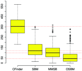
Figure 6: $L_{2}$ distance $d(\mathbf{P},\hat{\mathbf{P}})$ over the $100$ samples of networks with community structures and stars, for CFinder, SBM, MMSB and OSBM. Measures how well the underlying cluster assignment structure has been retrieved.

In this set of experiments we considered networks with more complex topologies. As shown, in Table 3 and in Figure 6, the results of CFinder dramatically degrade while those of OSBM remain more stable. Indeed, the median of the $L_{2}$ distances $d(\mathbf{P},\hat{\mathbf{P}})$ over the $100$ samples is equal to $43$ for OSBM, while it is equal to $354.5$ for CFinder. This can be easily explained since CFinder only looks for community structures of adjacent $k$-cliques, and cannot retrieve classes with low intra connection probabilities. Conversely, OSBM uses a $Q\times Q$ real matrix $\mathbf{W}$ and two real vectors $\mathbf{U}$ and $\mathbf{V}$ of size $Q$ to model the intra and inter connection probabilities. No assumption is made on these matrix and vectors such that OSBM can take heterogeneous and complex topologies into account. As for CFinder, the results of MMSB degrade, although they remain better than SBM. As for the previous Section, MMSB retrieves the clusters well but misclassifies the overlaps more frequently when considering networks with community structures and stars.

6.2 French political blogosphere

We consider the French political blogosphere network and we focus on a subset of 196 vertices connected by 2864 edges. The data consists of a single day snapshot of political blogs automatically extracted on the 14th of October 2006 and manually classified by the “Observatoire Présidentielle project” [Zanghi, Ambroise and Miele (2008)]. Nodes correspond to hostnames and there is an edge between two nodes if there is a known hyperlink from one hostname to another. The four main political parties which are present in the data set are the UMP (french “republican”), UDF (“moderate” party), liberal party (supporters of economic-liberalism) and PS (french “democrat”). Therefore, we applied our algorithm with $Q=4$ clusters and we obtained the results presented in Figure 7 and Table 4.

Figure 7: Classification of the blogs into $Q=4$ clusters using OSBM. The entry $(i,j)$ of the matrix describes the number of blogs associated to the $j$th political party (column) and classified into cluster $i$ (row). Each entry distinguishes blogs which belong to a unique cluster from overlaps (single membership blogs $+$ overlaps). The last row corresponds to the null component.

=250pt 3.89 $-$0.17 $-$0.54 $-$0.70 $-$0.70 0.17 $-$2.47 $-$0.40 $-$0.84 $-$0.40 0.55 $-$0.40 $-$4.43 $-$0.85 $-$0.38 $-$0.70 $-$0.84 $-$0.85 $-$1.660. $-$0.87 $-$0.70 $-$0.40 $-$0.38 $-$0.870. $-$3.60

Table 4: The estimated $\widetilde{\mathbf{W}}$ matrix for the classification of the blogs into $Q=4$ clusters using OSBM. The $4\times 4$ matrix on the top left-hand side represents the $\mathbf{W}$ matrix, while the vectors on the top right-hand side and bottom left-hand side represent the vectors $\mathbf{U}$ and $\mathbf{V}^{\top}$ respectively. The remaining term corresponds to the bias. The diagonal of $\mathbf{W}$ indicates that blogs have a heavy tendency to connect to blogs of the same class. Blogs of cluster 1 (UMP) have also a positive tendency to connect to blogs of clusters 2 (UDF) and 3 (liberal party). Conversely, blogs of cluster 4 (PS), representing the left wing, are more isolated in the network

First, we notice that the clusters we found are highly homogeneous and correspond to the well-known political parties. Thus, cluster 1 contains 35 blogs among which 33 are associated to UMP, while cluster 2 contains 39 blogs among which 30 are related to UDF. Similarly, it follows that cluster 3 corresponds to the liberal party and cluster 4 to PS. We found nine overlaps. Thus, three blogs associated to UMP belong to both clusters 1 (UMP) and 2 (UDF). This is a result we expected since these two political parties are known to have some relational ties. Moreover, a blog associated to UDF belongs to both clusters 1 (UMP) and 4 (PS), while another UDF blog belongs to clusters 2 (UDF) and 4 (PS). This can be easily understood since UDF is a moderate party. Therefore, it is not surprising to find UDF blogs with links with the two biggest political parties in France, representing the left and right wings. Very interestingly, among the nine overlaps we found, four of them correspond to blogs of political analysts. Thus, a blog overlaps clusters 1 (UMP) and 4 (PS). Another one overlaps clusters 2 (UDF), 3 (liberal party) and 4 (PS). Finally, the two last blogs of political analysts overlap clusters 2 (UDF) and 4 (PS).

We ran CFinder and we used the criterion [Palla et al. (2005)] they proposed to select $k$ (see Section 1). Thus, we ran the software for various values of $k$ and we found $\hat{k}=7$. Lower values lead to giant components which smear the details of the network. Conversely, for higher values, the communities start disintegrating. Using $\hat{k}$, we uncovered $11$ clusters which correspond to sub-clusters of the clusters we found using OSBM. For instance, cluster 3 (liberal party) was split into two clusters, whereas cluster 4 (PS) was split into three. Indeed, while OSBM predicted that the connection profiles of these sub-clusters were very similar and therefore should be merged, CFinder could not uncover any $k$-clique community, that is, a union of fully connected sub-graphs of size $k$, containing these sub-clusters. Note that using CFinder, we retrieved the overlaps uncovered by our algorithm. CFinder did not classify 95 blogs.

We also clustered the blogs of the network using MMSB and SBM. As previously, for both models, we used $Q+1$ clusters and we identified the class of outliers. The results of MMSB are presented in Figure 8. Overall, we can notice that MMSB led to similar clusters as OSBM, although cluster 4 is less homogeneous in MMSB than in OSBM. We found eight overlaps using MMSB and we emphasize that five of them correspond exactly to the one found with our approach. Thus, the model retrieved two among the three UMP blogs overlapping clusters 1 (UMP) and 2 (UDF). Moreover, MMSB uncovered the UDF blog overlapping clusters 1 (UMP) and 4 (PS), as well as the blog of political analysts overlapping clusters 2 (UDF), 3 (liberal party) and 4 (PS). It also retrieved the blog of political analysts overlapping clusters 1 (UMP) and 4 (PS). Finally, the results of SBM are presented in Figure 9. Again, the clusters found by this approach are very similar to the one uncovered by OSBM. However, because SBM does not allow each vertex to belong to multiple clusters, it misses a lot of information in the network. In particular, while some of the blogs of political analysts are viewed as overlaps by OSBM, because of their relational ties with the different political parties, they are all classified into a single cluster by SBM.

Figure 8: Classification of the blogs into $Q=5$ clusters using MMSB. The entry $(i,j)$ of the matrix describes the number of blogs associated to the $j$th political party (column) and classified into cluster $i$ (row). Each entry distinguishes blogs which belong to a unique cluster from overlaps (single membership blogs $+$ overlaps). Cluster 5 corresponds to the class of outliers.

Figure 9: Classification of the blogs into $Q=5$ clusters using SBM. The entry $(i,j)$ of the matrix describes the number of blogs associated to the $j$th political party (column) and classified into cluster $i$ (row). Cluster 5 corresponds to the class of outliers.

Table 5: Classification of the operons into $Q=6$ clusters. Operons in bold belong to multiple clusters

Cluster	Size	Operons
1	02	STE12 TEC1
2	33	YBR070C MID2 YEL033W SRD1 TSL1 RTS2 PRM5 YNL051W PST1
		YJL142C SSA4 YGR149W SPO12 YNL159C SFP1 YHR156C YPS1
		YPL114W HTB2 MPT5 SRL1 DHH1 TKL2 PGU1 YHL021C RTA1
		WSC2 GAT4 YJL017W TOS11 YLR414C BNI5 YDL222C
3	02	MSN4 MSN2
4	32	CPH1 TKL2 HSP12 SPS100 MDJ1 GRX1 SSA3 ALD2 GDH3 GRE3
		HOR2 ALD3 SOD2 ARA1 HSP42 YNL077W HSP78 GLK1 DOG2
		HXK1 RAS2 CTT1 HSP26 TPS1 TTR1 HSP104 GLO1 SSA4 PNC1
		MTC2 YGR086C PGM2
5	02	YAP1 SKN7
6	19	YMR318C CTT1 TSA1 CYS3 ZWF1 HSP82 TRX2 GRE2 SOD1 AHP1
		YNL134C HSP78 CCP1 TAL1 DAK1 YDR453C TRR1 LYS20 PGM2

6.3 Saccharomyces cerevisiae transcription network

We consider the yeast transcriptional regulatory network described in Milo et al. (2002) and we focus on a subset of 197 vertices connected by 303 edges. Nodes of the network correspond to operons, and two operons are linked if one operon encodes a transcriptional factor that directly regulates the other operon. The network is made of three regulation patterns, each one of them having its own regulators and regulated operons. Therefore, using $Q=6$ clusters, we applied our algorithm and we obtained the results in Table 5.

First, we notice that clusters 1, 3 and 5 contain only two operons each. These operons correspond to hubs which regulate respectively the nodes of clusters 2, 4 and 6, all having a very low intra connection probability. To analyze our results, we used GOToolBox [Martin et al. (2004)] on each cluster. This software aims at identifying statistically over-represented terms of the Gene Ontology (GO) in a gene data set. We found that the clusters correspond to well-known biological functions. Thus, the nodes of cluster 2 are regulated by STE12 and TEC1 which are both involved in the response to glucose limitation, nitrogen limitation and abundant fermentable carbon source. Similarly, MSN4 and MSN2 regulate the nodes of cluster 4 in response to different stress such as freezing, hydrostatic pressure and heat acclimation. Finally, the nodes of cluster 6 are regulated by YAP1 and SKN7 in the presence of oxygen stimulus. Our algorithm was able to uncover two overlapping clusters (operons in bold in Table 5). Interestingly, contrary to the other operons of clusters 2, 4 and 6, which are all regulated by operons of a single cluster (clusters 1, 3 or 5), these overlaps correspond to co-regulated operons. Thus, SSA4 and TKL2 belong to clusters 2 and 4 since they are co-regulated by (STE12, TEC1) and (MSN4 and MSN2). Moreover, HSP78, CTT1 and PGM2 belong to clusters 4 and 6 since they are co-regulated by (MSN4, MSN2) and (YAP1, SKN7). It should also be noted that OSBM did not classify 112 operons which all have very low output and input degrees.

Because the network is sparse, we obtained very poor results with CFinder. Indeed, the network contains only one $3$-clique and no $k$-clique for $k>3$. Therefore, for $k=2$, all the operons were classified into a single cluster and no biological information could be retrieved. For $k=3$, only three operons were classified into a single class and for $k>3$ no operon was classified.

As previously, we ran MMSB and SMB with $Q+1$ clusters and we identified the class of outliers. Both approaches retrieved the six clusters found by OSBM. However, we emphasize that, contrary to the political blogoshpere network, MMSB did not uncover any overlap in the yeast transcriptional regulatory network.

As in Section 6.1, these results clearly illustrate the capacity of OSBM to retrieve overlapping clusters in networks with complex topological structures. In particular, in situations where networks are not made of community structures, while the results of CFinder dramatically degrade or cannot even be interpreted, OSBM seems particularly promising.

7 Conclusion

In this paper we proposed a new random graph model, the Overlapping Stochastic Block Model, which can be used to retrieve overlapping clusters in networks. We used global and local variational techniques to obtain a tractable lower bound of the observed log-likelihood and we defined an EM like procedure which optimizes the model parameters in turn. We showed that the model is identifiable within classes of equivalence and we illustrated the efficiency of our approach compared to other methods, using simulated data and real networks. Since no assumption is made on the matrix $\mathbf{W}$ and vectors $\mathbf{U}$ and $\mathbf{V}$ used to characterize the connection probabilities, the model can take very different topological structures into account and seems particularly promising for the analysis of networks. In the experiment section we set the number $Q$ of classes using a priori information we had about the networks. However, in future works, we believe it is crucial to develop a model selection criterion to estimate the number of classes automatically from the topology. We will also investigate introducing some priors over the model parameters to work in a full Bayesian framework.

References

- Airoldi et al. (2006) {binproceedings}[author] \bauthor\bsnmAiroldi, \bfnmE.\binitsE., \bauthor\bsnmBlei, \bfnmD.\binitsD., \bauthor\bsnmXing, \bfnmE.\binitsE. and \bauthor\bsnmFienberg, \bfnmS.\binitsS. (\byear2006). \btitleMixed membership stochastic block models for relational data with application to protein–protein interactions. In \bbooktitleProceedings of the International Biometrics Society Annual Meeting. \bmiscMontréal, Québec, Canada. \endbibitem
- Airoldi et al. (2007) {barticle}[author] \bauthor\bsnmAiroldi, \bfnmE.\binitsE., \bauthor\bsnmBlei, \bfnmD.\binitsD., \bauthor\bsnmFienberg, \bfnmS.\binitsS. and \bauthor\bsnmXing, \bfnmE.\binitsE. (\byear2007). \btitleMixed membership analysis of high-throughput interaction studies: Relational data. \bmiscAvailable at ArXiv e-prints. \endbibitem
- Airoldi et al. (2008) {barticle}[author] \bauthor\bsnmAiroldi, \bfnmE. M.\binitsE. M., \bauthor\bsnmBlei, \bfnmD. M.\binitsD. M., \bauthor\bsnmFienberg, \bfnmS. E.\binitsS. E. and \bauthor\bsnmXing, \bfnmE. P.\binitsE. P. (\byear2008). \btitleMixed membership stochastic blockmodels. \bjournalJ. Mach. Learn. Res. \bvolume9 \bpages1981–2014. \endbibitem
- Allman, Matias and Rhodes (2009) {barticle}[author] \bauthor\bsnmAllman, \bfnmE. S.\binitsE. S., \bauthor\bsnmMatias, \bfnmC.\binitsC. and \bauthor\bsnmRhodes, \bfnmJ. A.\binitsJ. A. (\byear2009). \btitleIdentifiability of parameters in latent structure models with many observed variables. \bjournalAnn. Statist. \bvolume37 \bpages3099–3132. \MR2549554 \endbibitem
- Bickel and Chen (2009) {binproceedings}[author] \bauthor\bsnmBickel, \bfnmP.J.\binitsP. and \bauthor\bsnmChen, \bfnmA.\binitsA. (\byear2009). \btitleA non parametric view of network models and Newman–Girvan and other modularities. \bbooktitleProc. Natl. Acad. Sci. USA \bvolume106 \bpages21068–21073. \endbibitem
- Blei, Ng and Jordan (2003) {barticle}[author] \bauthor\bsnmBlei, \bfnmD.\binitsD., \bauthor\bsnmNg, \bfnmA.Y.\binitsA. and \bauthor\bsnmJordan, \bfnmM.I.\binitsM. (\byear2003). \btitleLatent Dirichlet allocation. \bjournalJ. Mach. Learn. Res. \bvolume3 \bpages993–1022. \endbibitem
- Boer et al. (2006) {bmanual}[author] \bauthor\bsnmBoer, \bfnmP.\binitsP., \bauthor\bsnmHuisman, \bfnmM.\binitsM., \bauthor\bsnmSnijders, \bfnmT.A.B.\binitsT., \bauthor\bsnmSteglich, \bfnmC.E.G.\binitsC., \bauthor\bsnmWichers, \bfnmL.H.Y.\binitsL. and \bauthor\bsnmZeggelink, \bfnmE.P.H.\binitsE. (\byear2006). \btitleStOCNET: An open software system for the advanced statistical analysis of social networks, \bnoteVersion 1.7. \endbibitem
- Broyden et al. (1970) {barticle}[author] \bauthor\bsnmBroyden, \bfnmC.G.\binitsC., \bauthor\bsnmFletcher, \bfnmR.\binitsR., \bauthor\bsnmGoldfarb, \bfnmD.\binitsD. and \bauthor\bsnmShanno, \bfnmD. F.\binitsD. F. (\byear1970). \btitleBFGS method. \bjournalJ. Inst. Math. Appl. \bvolume6 \bpages76–90. \endbibitem
- Byrd et al. (1995) {barticle}[author] \bauthor\bsnmByrd, \bfnmR. H.\binitsR. H., \bauthor\bsnmLu, \bfnmP.\binitsP., \bauthor\bsnmNocedal, \bfnmJ.\binitsJ. and \bauthor\bsnmZhu, \bfnmC.\binitsC. (\byear1995). \btitleA limited memory algorithm for bound constrained optimization. \bjournalSIAM J. Sci. Comput. \bvolume16 \bpages1190–1208. \MR1346301 \endbibitem
- Chang (2010) {bmanual}[author] \bauthor\bsnmChang, \bfnmJ.\binitsJ. (\byear2010). \btitleThe lda package \bnoteVersion, 1.2. \endbibitem
- Daudin, Picard and Robin (2008) {barticle}[author] \bauthor\bsnmDaudin, \bfnmJ.-J.\binitsJ.-J., \bauthor\bsnmPicard, \bfnmF.\binitsF. and \bauthor\bsnmRobin, \bfnmS.\binitsS. (\byear2008). \btitleA mixture model for random graphs. \bjournalStatist. Comput. \bvolume18 \bpages173–183. \MR2390817 \endbibitem
- Estrada and Rodriguez-Velazquez (2005) {barticle}[author] \bauthor\bsnmEstrada, \bfnmE.\binitsE. and \bauthor\bsnmRodríguez-Velázquez, \bfnmJ. A.\binitsJ. A. (\byear2005). \btitleSpectral measures of bipartivity in complex networks. \bjournalPhys. Rev. E (3) \bvolume72 \bpages046105. \MR2202758 \endbibitem
- Everett and Borgatti (1998) {barticle}[author] \bauthor\bsnmEverett, \bfnmM.G.\binitsM. and \bauthor\bsnmBorgatti, \bfnmS.P.\binitsS. (\byear1998). \btitleAnalyzing clique overlap. \bjournalConnections \bvolume21 \bpages49–61. \endbibitem
- Fienberg and Wasserman (1981) {barticle}[author] \bauthor\bsnmFienberg, \bfnmS.E.\binitsS. and \bauthor\bsnmWasserman, \bfnmS.\binitsS. (\byear1981). \btitleCategorical data analysis of single sociometric relations. \bjournalSoc. Methodol. \bvolume12 \bpages156–192. \endbibitem
- Frank and Harary (1982) {barticle}[author] \bauthor\bsnmFrank, \bfnmO.\binitsO. and \bauthor\bsnmHarary, \bfnmF.\binitsF. (\byear1982). \btitleCluster inference by using transitivity indices in empirical graphs. \bjournalJ. Amer. Statist. Assoc. \bvolume77 \bpages835–840. \MR0686407 \endbibitem
- Fu and Banerjee (2008) {binproceedings}[author] \bauthor\bsnmFu, \bfnmQ.\binitsQ. and \bauthor\bsnmBanerjee, \bfnmA.\binitsA. (\byear2008). \btitleMultiplicative mixture models for overlapping clustering. In \bbooktitleProceedings of the IEEE International Conference on Data Mining \bpages791–796. \bmiscPisa, Italy. \endbibitem
- Girvan and Newman (2002) {binproceedings}[author] \bauthor\bsnmGirvan, \bfnmM.\binitsM. and \bauthor\bsnmNewman, \bfnmM. E. J.\binitsM. E. J. (\byear2002). \btitleCommunity structure in social and biological networks. \bbooktitleProc. Natl. Acad. Sci. USA \bvolume99 \bpages7821–7826. \MR1908073 \endbibitem
- Goldenberg et al. (2010) {barticle}[author] \bauthor\bsnmGoldenberg, \bfnmA.\binitsA., \bauthor\bsnmZheng, \bfnmA.X.\binitsA., \bauthor\bsnmFienberg, \bfnmS.E.\binitsS. and \bauthor\bsnmAiroldi, \bfnmE.M.\binitsE. (\byear2010). \btitleA survey of statistical network models. \bjournalFound. Trends Mach. Learn. \bvolume2 \bpages129–233. \endbibitem
- Griffiths and Ghahramani (2005) {binproceedings}[author] \bauthor\bsnmGriffiths, \bfnmT.\binitsT. and \bauthor\bsnmGhahramani, \bfnmZ.\binitsZ. (\byear2005). \btitleInfinite latent feature models and the Indian buffet process. \bbooktitleAdv. Neural Inform. Process. Syst. \bvolume18 \bpages475–482. \endbibitem
- Handcock, Raftery and Tantrum (2007) {barticle}[author] \bauthor\bsnmHandcock, \bfnmM. S.\binitsM. S., \bauthor\bsnmRaftery, \bfnmA. E.\binitsA. E. and \bauthor\bsnmTantrum, \bfnmJ. M.\binitsJ. M. (\byear2007). \btitleModel-based clustering for social networks. \bjournalJ. Roy. Statist. Soc. Ser. A \bvolume170 \bpages301–354. \MR2364300 \endbibitem
- Heller and Ghahramani (2007) {binproceedings}[author] \bauthor\bsnmHeller, \bfnmK.\binitsK. and \bauthor\bsnmGhahramani, \bfnmZ.\binitsZ. (\byear2007). \btitleA nonparametric Bayesian approach to modeling overlapping clusters. In \bbooktitleProceedings of the 11th International Conference on AI and Statistics. \bmiscSan Juan, Puerto Rico. \endbibitem
- Heller, Williamson and Ghahramani (2008) {binproceedings}[author] \bauthor\bsnmHeller, \bfnmK.\binitsK., \bauthor\bsnmWilliamson, \bfnmS.\binitsS. and \bauthor\bsnmGhahramani, \bfnmZ.\binitsZ. (\byear2008). \btitleStatistical models for partial membership. In \bbooktitleProceedings of the 25th International Conference on Machine Learning \bpages392–399. \bmiscHelsinki, Finland. \endbibitem
- Hoff, Raftery and Handcock (2002) {barticle}[author] \bauthor\bsnmHoff, \bfnmP. D\binitsP. D., \bauthor\bsnmRaftery, \bfnmA. E.\binitsA. E. and \bauthor\bsnmHandcock, \bfnmM. S.\binitsM. S. (\byear2002). \btitleLatent space approaches to social network analysis. \bjournalJ. Amer. Statist. Assoc. \bvolume97 \bpages1090–1098. \MR1951262 \endbibitem
- Hofman and Wiggins (2008) {barticle}[author] \bauthor\bsnmHofman, \bfnmJ.M.\binitsJ. and \bauthor\bsnmWiggins, \bfnmC.H.\binitsC. (\byear2008). \btitleA Bayesian approach to network modularity. \bjournalPhys. Rev. Lett. \bvolume100 \bpages258701. \endbibitem
- Holland, Laskey and Leinhardt (1983) {barticle}[author] \bauthor\bsnmHolland, \bfnmP. W.\binitsP. W., \bauthor\bsnmLaskey, \bfnmK. B.\binitsK. B. and \bauthor\bsnmLeinhardt, \bfnmS.\binitsS. (\byear1983). \btitleStochastic blockmodels: First steps. \bjournalSocial Networks \bvolume5 \bpages109–137. \MR0718088 \endbibitem
- Jeffery (1999) {barticle}[author] \bauthor\bsnmJeffery, \bfnmC.J.\binitsC. (\byear1999). \btitleMoonlighting proteins. \bjournalTrends Biochem. Sci. \bvolume24 \bpages8–11. \endbibitem
- Krivitsky and Handcock (2009) {bmanual}[author] \bauthor\bsnmKrivitsky, \bfnmP.N.\binitsP. and \bauthor\bsnmHandcock, \bfnmM.S.\binitsM. (\byear2009). \btitleThe latentnet package, \bnoteVersion 2.1-1. \endbibitem
- Krivitsky et al. (2009) {barticle}[author] \bauthor\bsnmKrivitsky, \bfnmP.N.\binitsP., \bauthor\bsnmHandcock, \bfnmM.S.\binitsM., \bauthor\bsnmRaftery, \bfnmA.E.\binitsA. and \bauthor\bsnmHoff, \bfnmP.D.\binitsP. (\byear2009). \btitleRepresenting degree distributions, clustering, and homophily in social networks with latent cluster random effects models. \bjournalSocial Networks \bvolume31 \bpages204–213. \endbibitem
- Lacroix, Fernandes and Sagot (2006) {barticle}[author] \bauthor\bsnmLacroix, \bfnmV.\binitsV., \bauthor\bsnmFernandes, \bfnmC.G.\binitsC. and \bauthor\bsnmSagot, \bfnmM.-F.\binitsM.-F. (\byear2006). \btitleMotif search in graphs: Application to metabolic networks. \bjournalTrans. Comput. Biol. Bioinform. \bvolume3 \bpages360–368. \endbibitem
- Latouche, Birmelé and Ambroise (2009) {binbook}[author] \bauthor\bsnmLatouche, \bfnmP.\binitsP., \bauthor\bsnmBirmelé, \bfnmE.\binitsE. and \bauthor\bsnmAmbroise, \bfnmC.\binitsC. (\byear2009). \btitleAdvances in Data Analysis, Data Handling, and Business Intelligence, Bayesian Methods for Graph Clustering \bpages229–239. \bpublisherSpringer, \bmiscBerlin, Heidelberg. \endbibitem
- Latouche, Birmelé and Ambroise (2010) {barticle}[author] \bauthor\bsnmLatouche, \bfnmP.\binitsP., \bauthor\bsnmBirmelé, \bfnmE.\binitsE. and \bauthor\bsnmAmbroise, \bfnmC.\binitsC. (\byear2010). \btitleSupplement A to “Overlapping stochastic block models with application to the French blogosphere network.” \bmiscDOI: 10.12.14/10-AOAS382SUPP. \endbibitem
- Martin et al. (2004) {barticle}[author] \bauthor\bsnmMartin, \bfnmD.\binitsD., \bauthor\bsnmBrun, \bfnmC.\binitsC., \bauthor\bsnmRemy, \bfnmE.\binitsE., \bauthor\bsnmMouren, \bfnmP.\binitsP., \bauthor\bsnmThieffry, \bfnmD.\binitsD. and \bauthor\bsnmJacq, \bfnmB.\binitsB. (\byear2004). \btitleGOToolBox: Functional analysis of gene datasets based on Gene Ontology. \bjournalGenome Biol. \bvolume5. \endbibitem
- Milo et al. (2002) {barticle}[author] \bauthor\bsnmMilo, \bfnmR.\binitsR., \bauthor\bsnmShen-Orr, \bfnmS.\binitsS., \bauthor\bsnmItzkovitz, \bfnmS.\binitsS., \bauthor\bsnmKashtan, \bfnmD.\binitsD., \bauthor\bsnmChklovskii, \bfnmD.\binitsD. and \bauthor\bsnmAlon, \bfnmU.\binitsU. (\byear2002). \btitleNetwork motifs: Simple building blocks of complex networks. \bjournalScience \bvolume298 \bpages824–827. \endbibitem
- Moreno (1934) {bbook}[author] \bauthor\bsnmMoreno, \bfnmJ.L.\binitsJ. (\byear1934). \btitleWho Shall Survive?: A New Approach to the Problem of Human Interrelations. \bpublisherNervous and Mental Disease Publishing, Washington, DC. \endbibitem
- Newman and Leicht (2007) {binproceedings}[author] \bauthor\bsnmNewman, \bfnmM.\binitsM. and \bauthor\bsnmLeicht, \bfnmE.\binitsE. (\byear2007). \btitleMixture models and exploratory analysis in networks. \bbooktitleProc. Natl. Acad. Sci. USA \bvolume104 \bpages9564–9569. \endbibitem
- Nowicki and Snijders (2001) {barticle}[author] \bauthor\bsnmNowicki, \bfnmK.\binitsK. and \bauthor\bsnmSnijders, \bfnmT. A. B.\binitsT. A. B. (\byear2001). \btitleEstimation and prediction for stochastic blockstructures. \bjournalJ. Amer. Statist. Assoc. \bvolume96 \bpages1077–1087. \MR1947255 \endbibitem
- Palla et al. (2005) {barticle}[author] \bauthor\bsnmPalla, \bfnmG.\binitsG., \bauthor\bsnmDerenyi, \bfnmI.\binitsI., \bauthor\bsnmFarkas, \bfnmI.\binitsI. and \bauthor\bsnmVicsek, \bfnmT.\binitsT. (\byear2005). \btitleUncovering the overlapping community structure of complex networks in nature and society. \bjournalNature \bvolume435 \bpages814–818. \endbibitem
- Palla et al. (2006) {bmanual}[author] \bauthor\bsnmPalla, \bfnmG.\binitsG., \bauthor\bsnmDerenyi, \bfnmI.\binitsI., \bauthor\bsnmFarkas, \bfnmI.\binitsI. and \bauthor\bsnmVicsek, \bfnmT.\binitsT. (\byear2006). \btitleCFinder the community/cluster finding program, \bnoteVersion 2.0.1. \endbibitem
- Snijders and Nowicki (1997) {barticle}[author] \bauthor\bsnmSnijders, \bfnmT. A. B.\binitsT. A. B. and \bauthor\bsnmNowicki, \bfnmK.\binitsK. (\byear1997). \btitleEstimation and prediction for stochastic blockmodels for graphs with latent block sturcture. \bjournalJ. Classification \bvolume14 \bpages75–100. \MR1449742 \endbibitem
- White, Boorman and Breiger (1976) {barticle}[author] \bauthor\bsnmWhite, \bfnmH.C.\binitsH., \bauthor\bsnmBoorman, \bfnmS.A.\binitsS. and \bauthor\bsnmBreiger, \bfnmR.L.\binitsR. (\byear1976). \btitleSocial structure from multiple networks. I. Blockmodels of roles and positions. \bjournalAmer. J. Soc. \bvolume81 \bpages730–780. \endbibitem
- Zanghi, Ambroise and Miele (2008) {barticle}[author] \bauthor\bsnmZanghi, \bfnmH.\binitsH., \bauthor\bsnmAmbroise, \bfnmC.\binitsC. and \bauthor\bsnmMiele, \bfnmV.\binitsV. (\byear2008). \btitleFast online graph clustering via Erdös–Renyi mixture. \bjournalPattern Recognition \bvolume41 \bpages3592–3599. \endbibitem