Information Theory and Renormalization Group Flows

Abstract

We present a possible approach to the study of the renormalization group (RG) flow based entirely on the information theory. The average information loss under a single step of Wilsonian RG transformation is evaluated as a conditional entropy of the fast variables, which are integrated out, when the slow ones are held fixed. Its positivity results in the monotonic decrease of the informational entropy under renormalization. This, however, does not necessarily imply the irreversibility of the RG flow, because entropy is an extensive quantity and explicitly depends on the total number of degrees of freedom, which is reduced. Only some size-independent additive part of the entropy could possibly provide the required Lyapunov function. We also introduce a mutual information of fast and slow variables as probably a more adequate quantity to represent the changes in the system under renormalization and evaluate it for some simple systems. It is shown that for certain real space decimation transformations the positivity of the mutual information directly leads to the monotonic growth of the entropy per lattice site along the RG flow and hence to its irreversibility.

I Introduction

Renormalization group (RG), which is a powerful instrument for analyzing different strongly coupled systems W (see also BBD for more recent reviews), is usually based upon an appropriate division of the whole set of variables into two subsets: so called “fast” and “slow” variables with subsequent elimination of the fast ones. The resulting slow system is usually expected to behave essentially in the same way as the initial one but with coupling constants changed. Successive application of this transformation results in a flow in the space of couplings. After each step of the RG transformation the information about exact values of fast variables is lost for the observer to whom only slow variables are available. It seems natural then to expect, that this information loss should lead to the irreversible character of the corresponding RG flow.

This irreversibility is a subject of an intensive study for several decades now, starting from the famous work of Zamolodchikov Z , who showed under certain assumptions that in two dimensions (2D) there exists a function on a space of coupling constants (a kind of Lyapunov function) which always decreases along the RG flow and at fixed points coincides with the central charge $c$ of corresponding conformal theories. “Irreversibility” here means that the flow in the space of couplings resembles that of a simple dissipative system with a given trajectory never returning back to its starting point, thus excluding limit cycles or more complex strange attractors. In 2D theories the $c$-theorem of Ref. Z states that the RG evolution is exactly of this type and looks like a simple monotonic flow downhill in the couplings’ space from fixed points with large $c$ to those with smaller values of the central charge.

Much work have been done in this direction and the $c$-theorem was studied in detail with its possible generalizations to higher dimensions (see e.g. c and references therein and also Ftheor for quite recent development). Still the interesting possibility that in general the flow may be more complicated, and may even exhibit chaotic behavior, like in case of many other nonlinear mappings, attracts some attention M (probably the first example of a chaotic RG flow was found for spin systems on hierarchical lattices h , see also Da ; D ). The models where such peculiarities are observed are however rather artificial, so that the question whether they could take place in more realistic cases remains somewhat unclear.

Though this problem is rather complicated mathematically it looks much simpler from the physical point of view. The Wilsonian RG transformation is designed in such a way that all finite dimensionless correlation lengths in a translationally invariant system always decrease W . To say this another way, all masses (measured in units of an ultra-violet cut-off) grow and it seems quite natural that the effective number of massless modes, (in 2D measured by the central charge $c$) cannot increase. The argument based on the growth of masses, though not completely rigorous, is quite general, hence something unusual, like limit cycles in the flow, may be expected only in some special systems with only infinite correlation lengths or with infinite number of correlation lengths which can be arbitrarily large (when we have e.g. a self-similar spectrum of masses converging to zero GW ). But in systems with finite number of well defined correlation lengths the RG flow should probably always be irreversible.

This argument however seems to be unrelated to the aforementioned information loss and information aspects probably play no role in the irreversibility, which may seem somewhat strange. Probably the most known attempt to study RG irreversibility using information theory tools is the approach of Ref. G1 ; G2 where the relative entropy was introduced in quantum field theory and some monotonicity theorems for it, as a function of relevant couplings, were proved and its relation to $c$-theorem was discussed.

In this paper we present a somewhat different, entirely information theory based approach to the problem of the RG flow, oriented more on discrete real space RG transformations in different lattice spin systems. Clearly, information-theoretic considerations are too general to lead to some non-trivial concrete results, but still, as we shall see below they may impose some restrictions on the possible character of the flow. First, in Section 2 we evaluate an exact amount of information loss for a single step of the renormalization as a kind of conditional entropy of fast variables (compare with L ). As one might expect, this information loss is equal to the decrease of entropy under the RG transformation. Thus it is possible to establish a general theorem about the monotonic decrease of the total entropy (and relative entropy as well) under general coarse graining as a result of information loss.

The monotonic decrease of entropy along the RG flow is neither something unusual (see e.g. Ro ) nor very interesting, because the entropy is proportional to the total number of degrees of freedom and should certainly decrease when some of them are integrated out. Hence this monotonic behavior does not directly lead to the irreversibility of the flow. An interesting thing may happen however, if the entropy of a finite system possesses an additive size-independent part. If this part of the entropy also decreases, as the total entropy does, then it may provide the proper Lyapunov function, because it does not explicitly depend on the number of variables and its change is entirely due to the flow of coupling constants. We will show that this takes place in 1D Ising model, where this subextensive part of the entropy is known as the “excess entropy” and was studied in detail as a measure of statistical complexity of spatial structures FC . This excess entropy equals to the mutual entropy of two halves of the system which is actually the reason why it decreases under coarse graining. Unfortunately we are unable to present a general theorem concerning the monotonicity of such excess entropy in higher dimensions.

It appears possible though to prove quite a different monotonicity theorem, but only for a certain class of real space lattice RG transformations, namely for decimations, when exactly half of variables are eliminated on each step. The proof is based on the analysis of a new quantity introduced in Section 3,—mutual information of slow and fast variables. Contrary to the information loss this mutual information shows how much information about eliminated fast variables is still present after a single step of the Wilsonian renormalization. The nonnegativity of the mutual information may alone impose some restrictions on the character of the flow leading to its irreversibility.

For the decimations of the aforementioned type in lattice models we will show that the entropy per lattice site monotonically grows as a result of the positivity of the mutual information of spins on two identical sublattices, one of which is eliminated in the course of the RG transformation. Therefore such decimation transformations, though they results in highly non-linear mappings, always lead to irreversible flows in the space of couplings. Simple examples of such a behavior are discussed in Section 4, where one- and two-dimensional classical spin models and also the continuum limit Gaussian model are considered. Note, however, that the theorem holds true only for systems with real actions, when information theory can be applied, while e.g. it is not valid for the Ising model with complex external magnetic field where the decimation RG flow is known to be chaotic D . The theorem is also invalid for spin models on hierarchical lattices h , because decimations are not associated there with decomposition of these finite and inhomogeneous lattices into two identical sublattices.

The entropy per site growth may seem somewhat unexpected, because it takes place not only in the trivial case, when the flow goes to the high-temperature fixed point, but even when we start from points located in the ordered phase. RG trajectories that start from points below the phase transition can never end in the fully disordered trivial fixed point, since for decimation the mean magnetization is conserved along the flow, but nevertheless the entropy per site (and hence the amount of disorder) will always grow. This is a peculiar feature of the decimation and does not take place for other possible renormalization schemes, like e.g. the majority rule block spin transformation also discussed in Section 4.

II Information loss and the RG flow

Suppose that we somehow manage to divide our variables into “fast” $\psi$ and “slow” ones $\eta$. For the Wilsonian momentum space RG the fast variables are high Fourier harmonics of the fields, but for real space renormalization in lattice systems $\psi$’s are just spins on some sublattice, so that they are not actually “fast” in any sense. Still we will use these names to distinguish degrees of freedom to be integrated out and those that remain. The partition function is given by the sum over all fields, which symbolically may be written as

$$Z=\sum_{\psi,\eta}\exp\left(-S(\psi,\eta)\right),$$ (1)

where $S(\psi,\eta)$ is the action (or energy divided by temperature for classical lattice systems). The fields normally depend on all space-time coordinates, so that the sums in Eq. (1) are actually path integrals, properly regularized. Now, the first step of the RG transformation is to integrate out the fast variables $\psi$ to obtain an effective action for the slow ones, $S^{\prime}(\eta)$, defined by

$$\exp\left(-S^{\prime}(\eta)\right)=\sum_{\psi}\exp\left(-S(\psi,\eta)\right)$$ (2)

This transformation is then repeated many times resulting in the RG flow of the corresponding actions (or coupling constants if the form of the action is fixed).

II.1 Information loss and entropy

Certainly, after the fast variables are eliminated, information about their exact values is lost. One can ask then, what is the precise amount of the information loss. For a moment let us fix the slow variables $\eta$, then the conditional probability for $\psi$ (normalized to unity) is

$$p(\psi|\eta)=\exp\left(-S(\psi,\eta)+S^{\prime}(\eta)\right),$$ (3)

$$\sum_{\psi}p(\psi|\eta)=1.$$

It seems natural then to define the information (measured in ‘nats’) related to some field configuration $\psi$ in the fixed background $\eta$ by the usual Shannon formula

$$I_{\psi}=-\ln p(\psi|\eta),$$ (4)

and the information loss after the fields $\psi$ are integrated out as an average of (4) over the distribution (3)

$$\langle I_{\psi}\rangle=-\sum_{\psi}p(\psi|\eta)\ln p(\psi|\eta)$$ (5)

This quantity still depends on the chosen configuration of the slow fields $\eta$. Actually $\langle I_{\psi}\rangle$ is similar, in a sense, to the Boltzmann entropy of a ‘macrostate’ specified by the coarse-grained variables $\eta$. Indeed, in case of ‘equipartition’, when $p(\psi|\eta)$ does not depend on $\psi$ in some domain of fast variables the information loss Eq.(5) is just the logarithm of the number of ‘microstates’ corresponding to a given macrostate.

We propose then that the total information loss $\delta I$ is an average of $\langle I_{\psi}\rangle$ over all configurations of $\eta$ with the corresponding weight $p(\eta)=1/Z\exp(-S^{\prime})$, i.e.

$$\delta I=-\sum_{\eta}p(\eta)\sum_{\psi}p(\psi|\eta)\ln p(\psi|\eta).$$ (6)

This is obviously the conditional entropy $H(\psi|\eta)$ of two sets of random variables $\psi$ and $\eta$ well known from the information theory Cov . This is the average entropy of the fast variables given the state of the slow subsystem. The conditional entropy of this kind usually measures the amount of information loss in a noisy channel when $\psi$ is an input signal and $\eta$ is an output. One can also view the RG transformation as an action of a smoothing filter, then $\delta I$ is the information loss due to smoothing. The conditional entropy as a measure of information loss also have been introduced in Ref. L where a coarse graining of polymer configurations was considered.

The above estimate of the information loss introduces a somewhat new paradigm of renormalization. We see now that it is possible to view the fast fields $\psi$ as an input signal, not directly available to a receiver, while the slow field $\eta$ is an output. After renormalization only the output signal is available and one can only try to restore the input signal more or less accurately. This is a typical situation of a signal transmission through a noisy channel where information loss may be estimated as a conditional entropy (6). But this analogy suggests that it may probably be of more use to discuss not only the information loss but also the information that is preserved, i.e. information about fast variables that is stored in the action for the slow ones (see Section 3).

Substituting the probability distributions into Eq. (6) we easily obtain

$$\delta I=H(\psi|\eta)=\langle S\rangle_{S}-\langle S^{\prime}\rangle_{S^{\prime}}=H-H^{\prime},$$ (7)

where the brackets $\langle\ldots\rangle$ mean the average over the fields with the corresponding actions (clearly, for continuous theory some regularization is required for these formulas to make sense), the initial informational entropy $H$ of the distribution $p(\psi,\eta)$ is given by

$$H=-\sum_{\eta,\psi}p(\psi,\eta)\ln p(\psi,\eta)=\langle S\rangle_{S}+\ln Z,$$ (8)

where

$$p(\eta,\psi)=\frac{1}{Z}\exp(-S(\eta,\psi))$$ (9)

and the entropy of the slow field $H^{\prime}=H(\eta)$ is given by the same formula with $p(\eta,\psi)\rightarrow p(\eta)$ and $S\rightarrow S^{\prime}$. Recall that our RG transformation is defined in such a way that the partition function $Z$ remains unchanged. Also note that the new action $S^{\prime}$, defined by (2), always contains an additive constant term, but it does not contribute to the entropy and may be ignored in the evaluation of $H^{\prime}$.

The Shannon entropy $H$ used here is the entropy of the fluctuating fields and it measures in fact how large these fluctuations are. For a classical system $H$ coincides with its thermodynamic entropy $H_{T}$, but in quantum systems (in the continuum limit) they are different, because $H_{T}$ is related to fluctuations in occupation of energy levels and not to that of fields as functions of space-time coordinates. While $H$ is dominated by an ultra-violet divergent “bulk” contribution, proportional to the space-time volume, the quantum thermodynamic entropy $H_{T}$ looks, in a sense, as a finite-size correction to a leading term in $H$. Indeed, for example, for a 2D system on a large cylinder of length $L$ and circumference $\beta$ which may be viewed as a 1D quantum system at a temperature $T=1/\beta$ we have $\ln Z\sim L\beta$ and the same is true for $H$, but this bulk term obviously does not contribute to the thermodynamic entropy $H_{T}=\partial(T\ln Z)/\partial T$. Hence non-zero $H_{T}$ arises only from finite size corrections to $\ln Z$ (see Section 4.5 for another example).

Thus the information loss $\delta I$ is merely the difference of the initial entropy $H=H(\psi,\eta)$ and the entropy of the remaining slow variables $H(\eta)$. For discrete variables $\eta$, $\psi$ (e.g. for classical spin systems) both entropies and the conditional entropy are always nonnegative, $H\geq 0$, $H^{\prime}\geq 0$ and $H(\psi|\eta)\geq 0$ and hence

$$H\geq H^{\prime},$$ (10)

which means that the entropy of the remaining variables decreases along the RG flow.

At first glance this decrease of entropy may seem strange, since if the flow is e.g. directed toward the high temperature fixed point the system obviously gets more disordered after renormalization. Recall, however, that it is the total entropy, an extensive quantity proportional to the system size, that decreases according to Eq. (10) and this decrease is mainly due to the fact that the total number of variables is reduced after some of them are integrated out. For example, in large lattice systems $H\simeq Nh$, where $N$ is the number of sites which decreases under real space RG transformation. The entropy per lattice site $h$ which is a more adequate measure of disorder may well increase along the RG flow.

Therefore the information loss $\delta I$ is not very informative about the change in physics under renormalization and the monotonic decrease of $H$ does not in general give rise to a proper Lyapunov function defined on the space of coupling constants.

This is not very surprising because the total information loss is a rather crude characteristic of the RG transformation. An interesting possibility still remains, that some part of this information loss may provide the required monotonic function. The most natural choice probably would be some volume-independent additive part in $H$ for a finite system, something that may be called e.g. information about boundary conditions. An example of such a function will be explicitly presented in section 4.1 for the one-dimensional Ising model. How to obtain possible extension of this result to higher dimensions is however not clear.

To conclude this subsection it should be mentioned, that for continuous field variables when we deal not with true probabilities but probability distributions and sums are replaced by integrals, direct application of the above formulas may lead to negative values of entropies Cov and to negative $\delta I$ which certainly is not acceptable. To avoid this one should either somehow make the variables $\eta$, $\psi$ discrete (“digitize” them) or better use some other quantities, which do not suffer from such a drawback, like e.g. the relative entropy.

II.2 Relative entropy

Relative entropy is the basic concept of the approach to renormalization developed in a series of papers G1 ; G2 . For the sake of completeness we present here a short discussion of its properties with regard to the Wilsonian RG transformation.

Consider some statistical system with variables $\phi$, and two probability distributions $\mu(\phi)$ and $\nu(\phi)$. Then we may introduce the relative entropy $H_{rel}$ as the so called Kullback-Leibler distance (divergence) $D(\mu||\nu)$ between these probability distributions

$$H_{rel}=D(\mu||\nu)=\sum_{\phi}\mu(\phi)\ln\frac{\mu(\phi)}{\nu(\phi)}$$ (11)

This distance, though not symmetric, is nonnegative even for continuous $\phi$ and $H_{rel}=0$ for $\mu=\nu$.

Now, the main idea of the approach G1 is to consider probability distributions corresponding to two actions $S_{1}$ and $S_{2}$ which differ by the values of coupling constants, and to study the relative entropy $H_{rel}=D(p_{1}||p_{2})$ where $p_{1}\sim\exp(-S_{1})$ and $p_{2}\sim\exp(-S_{2})$, and then choose $p_{2}$ to correspond to a RG fixed point distribution. Thus physically this $H_{rel}$ measures how far our system with the action $S_{1}$ is from a given fixed point. Then we expect the relative entropy to behave monotonically under the change of the coupling constant, corresponding e.g. to some relevant perturbation of the fixed point.

In fact, some rather general results are known about the behavior of $H_{rel}$ under a coarse-graining. Let us proceed as usual and decompose the whole set of fields $\phi$ into fast $\psi$ and slow ones $\eta$. If we introduce conditional probability $p(\psi|\eta)$ (normalized to unity $\sum_{\psi}p(\psi|\eta)=1$) and make use of $p(\psi,\eta)=p(\eta)p(\psi|\eta)$ we can write the following chain of equalities

$$H_{rel} = \sum_{\psi,\eta}p_{1}(\psi,\eta)\ln\frac{p_{1}(\psi,\eta)}{p_{2}(\psi,\eta)}=$$ (12)

$$= \sum_{\psi,\eta}p_{1}(\eta)p_{1}(\psi|\eta)\ln\frac{p_{1}(\eta)p_{1}(\psi|\eta)}{p_{2}(\eta)p_{2}(\psi|\eta)}=$$

$$= \sum_{\eta}p_{1}(\eta)\ln\frac{p_{1}(\eta)}{p_{2}(\eta)}+$$

$$+ \sum_{\eta}p_{1}(\eta)\sum_{\psi}p_{1}(\psi|\eta)\ln\frac{p_{1}(\psi|\eta)}{p_{2}(\psi|\eta)}.$$

The first term in the resulting expression is obviously the relative entropy after renormalization, $H^{\prime}_{rel}$, while the last term is known in information theory as a conditional relative entropy which is always nonnegative Cov . Hence we have

$$H_{rel}\geq H^{\prime}_{rel}$$ (13)

This result, as well as the derivation of Eq. (12), is in fact widely known and usually referred to as a decrease of relative entropy under any kind of coarse-graining Cov . The decrease of relative entropy for continuum Gaussian model with lowering the ultra-violet cutoff G1 is just one example of this general phenomenon.

One can also view Eq. (12) as a generalization of the expression (7) for the information loss. Then the last term in Eq. (12) may probably be called “conditional information loss”. Since this is nonnegative also for continuous variables it looks more preferable for quantum field theory, than the information loss from the previous subsection.

Unfortunately inequality (13) for the relative entropy is also not very useful because normally $H_{rel}$ is an extensive quantity and its monotonic decrease again may be attributed to the reduction in the number of degrees of freedom (effective shrinking of the system under renormalization) and it is a specific quantity $h_{rel}=H_{rel}/N$, where $N$ is e.g. a number of lattice sites, which is physically relevant. A more careful analysis shows however that $H_{rel}$ is much better that entropy $H$ or similar quantities and possesses interesting monotonicity properties with respect to couplings (see Refs. G1 ; G2 for details). For example, close to a critical point with a diverging dimensionless correlation length $\xi$ the relative entropy taken with respect to the fixed point distribution in many cases behaves as $\sim N/{\xi}^{d}$ (for $d$-dimensional lattice system) and is universal, depending not on the total number of variables, but only on the number of blocks of size $\xi$. This means that relative entropy does not contain redundant “low-level” information. When this is true $h_{rel}\sim 1/\xi$ is obviously monotonic along the Wilsonian RG flow, which is a particular example of how the informational “distance” grows on a trajectory moving away from the unstable fixed point.

If we take $\nu$ in (11) to be a uniform distribution $\nu={\rm const}$, then $H_{rel}=-\ln\nu-H$, where $H$ is the entropy of a given distribution $\mu$. Therefore, if the first term $\ln\nu$ remains constant, the decrease of the relative entropy under a coarse-graining is usually related to the growth of the entropy $H$ Cov . In our case, however, the first term also changes, because $\ln\nu\sim N$ due to normalization condition for $\nu$ and therefore $H_{rel}$ and $H$ both decrease.

III Mutual information of fast and slow variables

We now introduce another information-related quantity, the so called mutual information of the fast and slow variables, which seems to be free of the aforementioned drawbacks. We shall demonstrate now that the nonnegativity of this mutual information may itself impose some restriction on the RG flow.

To define this mutual information, we need to perform a transformation opposite, in a sense, to the usual RG transform of Eq. (2), namely to integrate out the slow variables. This will result in an effective action $\tilde{S}^{\prime}$ for the fast variables $\psi$, their probability distribution being $p(\psi)\sim\exp(-\tilde{S}^{\prime}(\psi))$, and the corresponding entropy will be denoted by $H(\psi)$. Then the mutual information of two sets of variables $\psi$ and $\eta$ is defined as

$$I=\sum_{\psi,\eta}p(\eta,\psi)\ln\left[\frac{p(\eta,\psi)}{p(\eta)p(\psi)}\right]$$ (14)

where $p(\eta,\psi)=1/Z\exp(-S)$ is the probability distribution for the initial system (joint probability for $\eta$ and $\psi$ variables).

The mutual information is certainly a kind of relative entropy which in our case measures the “distance” $D(p(\psi,\eta)||p(\psi)p(\eta))$ between the original system and some hypothetic one where fast and slow variables are independent, but described by their true corresponding effective actions, i.e. $\mu=p(\psi,\eta)$ and $\nu=p(\psi)p(\eta)$ in Eq. (11).

Substituting expressions for probabilities in terms of actions one can easily derive the well known formulas from elementary information theory

$$I=H(\eta)-H(\eta|\psi)=H(\psi)-H(\psi|\eta)=$$

$$=[H(\eta)+H(\psi)]-H(\psi,\eta)$$ (15)

Here $H(\psi|\eta)=\delta I$ is the information loss after the normal RG transformation and $H(\eta|\psi)$ is the information loss after elimination of the slow variables, or if we adopt the view that renormalization is the information transmission through the noisy channel $\psi\rightarrow\eta$, then $H(\eta|\psi)$ is a measure of the noise Cov .

In bipartite systems the mutual information is nonnegative and is known to measure the information about one subsystem stored in the other Cov (for independent subsystems $I=0$), i.e. in our case it shows what amount of information about the fast fields $\psi$ is still contained in the effective action $S^{\prime}(\eta)$. Since usually RG transformation results in the change of coupling constants it seems natural to think that the information about the eliminated fast variables is now hidden in the new values of these constants. Therefore $I$ should be directly related to the RG flow of the coupling constants.

Note also that $I$ is represented in the last equation of Eq. (III) as a difference of two quantities with roughly the same size dependence, so that it should not be so sensitive to the reduction of degrees of freedom under the RG transformation.

While in general $I$ is more difficult to calculate than the entropy, there exists an interesting situation when $H(\psi)=H(\eta)=H^{\prime}$ and $I=2H^{\prime}-H$. This happens e.g. for some decimation transformations in lattice systems, when the system is divided into two identical sub-lattices (see next Section) and exactly half of variables (those on one sub-lattice) are integrated out. For large enough system with $N$ sites we may write $H=Nh$ and $H^{\prime}=(N/2)h^{\prime}$ where $h$ and $h^{\prime}$ are the entropies per lattice site before and after the renormalization. Then

$$I=N(h^{\prime}-h)\geq 0\qquad\Rightarrow\qquad h^{\prime}\geq h$$ (16)

and hence the condition $I\geq 0$ directly leads to the growth of the entropy per lattice site along the RG trajectory.

This means that such decimations are always irreversible, but suggests that corresponding RG flows do not have fixed points for finite generic values of couplings. Indeed, if there exists a fixed point then at this point $h=h^{\prime}$ and hence the bulk mutual information $I$ is zero. But this means that spins on two sub-lattices are essentially uncorrelated and remain uncorrelated under renormalization, which seems impossible for realistic spin systems with reasonable finite interactions. Note, that this does not imply that decimation does not have nontrivial fixed points at all, but such fixed points (apart from the trivial high-temperature one) should probably lie at the “boundary” of the parameter space, when some couplings are set to infinity, as one can see e.g. in the classical spin-1 model on a line spo (see also section 4.2).

The absence of a nontrivial fixed point corresponding to the phase transition for pure decimation in 2D Ising model have been noticed already in W ; KH and was related to the fact that decimation does not eliminates only “short range” correlations but inevitably sums over some long-range behavior SB , i.e. it is actually not a good RG transformation.

Let us now take a look at some simple examples.

IV Examples of the informational approach

IV.1 One-dimensional Ising model.

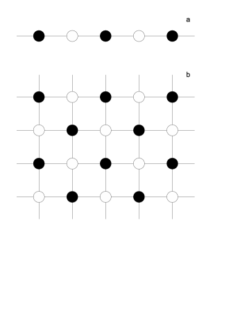
Figure 1: Decimation transformations on (a) one-dimensional lattice and (b) two-dimensional square lattice. Spins on white lattice sites are summed away.

The classical one-dimensional ferromagnetic Ising model is the most known example of the RG transformation which here can be performed exactly. The model is defined on a lattice with $N$ sites and the initial action is given by $S=-K\sum_{i}s_{i}s_{i+1}$, where $s_{i}=\pm 1$. The real space RG procedure (decimation) is defined as follows: we decompose the lattice into two sub-lattices and sum over spins on one sublattice KH (see Fig. 1a). The resulting model is again of the Ising type with $K\rightarrow K^{\prime}$, with twice the initial lattice spacing and $N/2$ sites. The entropy $H$ is here the true entropy of the Ising model and the information loss, defined by Eq. (7), is

$$\delta I=Nh(K)-\frac{N}{2}h(K^{\prime}),$$ (17)

where $h(K)$ is the entropy per lattice site

$$h(K)=-K\tanh K+\ln(2\cosh K),$$ (18)

and

$$K^{\prime}=(1/2)\ln(\cosh(2K)).$$ (19)

The RG flow is very simple since the running coupling constant $K$ flows from the zero temperature fixed point $K=\infty$ to the high temperature one at $K=0$.

Though $K^{\prime}$ decreases during the RG procedure and $h(K^{\prime})>h(K)$ it is easy to verify that $\delta I$ is always positive, has its maximum $(N/2)\ln 2$ at $K=0$ and then monotonically decreases to zero as $K\rightarrow\infty$.

It is interesting that for large $K,K^{\prime}$ the information loss can be obtained independently, so that Eq. (17) can be used to derive $K^{\prime}$. Indeed, if $K\rightarrow\infty$ most probable spin configurations are that of well separated kinks (domain walls). If a spin, which is eliminated, falls inside a domain, no information is lost, because its value does not fluctuate at large $K$ and is completely determined by adjacent spins. But a spin that lies on a domain wall is completely unconstrained and hence the information loss is $\ln 2$. Since there are on the average $N\exp(-2K)$ kinks at $K\rightarrow\infty$ we conclude that

$$\delta I\simeq N\exp(-2K)\ln 2+\ldots,$$ (20)

where dots indicate terms of higher order in $\exp(-2K)$. At large $K$ the leading term in entropy is $h(K)\simeq\hbox{$(2K+1)$}\exp(-2K)$ hence Eq. (17) results in

$$(2K+1-\ln 2)\exp(-2K)=(K^{\prime}+\frac{1}{2})\exp(-2K^{\prime}),$$ (21)

which has the solution

$$K^{\prime}=K-\frac{1}{2}\ln 2+\ldots.$$ (22)

This is the correct expression for the renormalized coupling at $K\rightarrow\infty$ and we see now that $\ln 2$ here is in fact of informational origin.

Now we discuss the relative entropy Eq. (11) of the Ising model at some coupling $K_{1}$ taken with respect to the state at a different coupling $K_{2}$. The general formula, derived in G1 states that

$$H_{rel}=W(K_{1})-W(K_{2})-(K_{1}-K_{2})\frac{\partial W(K_{1})}{\partial K_{1}},$$ (23)

where

$$W=-\ln Z.$$ (24)

In our case $W(K)=-N\ln(2\cosh K)$ and hence

$$H_{rel}(K_{1},K_{2})=-N\ln\frac{\cosh K_{1}}{\cosh K_{2}}+N(K_{1}-K_{2})\tanh K_{1}.$$ (25)

We can look now at some limiting cases. First consider the entropy relative to the high temperature fixed point $K_{2}=0$. Then

$$H_{rel}(K,0)=N(\ln 2-h(K))=N\ln 2-H.$$ (26)

One can easily see that $H_{rel}$ decreases under the RG transformation when $K\rightarrow K^{\prime}$ and $N\rightarrow N/2$ and $h_{rel}=H_{rel}/N$ also tends to zero.

The entropy relative to the zero temperature fixed point should be obtained in the limit $K_{2}\rightarrow\infty$ but the limiting expression diverges. Fortunately, we can take $K_{1}=\infty$ which is almost the same for our purposes. Then

$$H_{rel}(\infty,K)=N[-K+\ln(2\cosh K)].$$ (27)

Again the total relative entropy monotonically decreases along the RG flow as the general proof suggests, but now $h_{rel}$ increases from zero to $\ln 2$. Close to the critical point

$$H_{rel}(\infty,K)\simeq N\exp(-2K)=2N/\xi,\qquad K\rightarrow\infty$$ (28)

where $\xi\simeq 1/2\exp(2K)$ is the correlation length. Thus, in this limit $H_{rel}$ is not changed by the RG transformation $\xi\rightarrow\xi/2$, $N\rightarrow N/2$ and actually measures the number of blocks of size $\xi$ as the general analysis suggests G1 ; G2 .

This example clearly illustrates that $H_{rel}$ always decreases, but this behavior is in part due to the effective shrinking of the system $N\rightarrow N/2$ and implies only that $h_{rel}(K^{\prime})\leq 2h_{rel}(K)$. The relative entropy per lattice site $h_{rel}$ is more useful because it really measures the “distance” from the fixed points and its evolution is related to the direction of the flow. Since here the RG flow is from the zero temperature fixed point to the high temperature one, $h_{rel}(K,0)$ decreases while $h_{rel}(\infty,K)$ monotonically grows (as $1/\xi$ close to the critical point).

It is easy also to calculate the mutual information $I$ for this model. Since the two sublattices are identical and similar to the original one, $H(\psi)=H(\eta)=H^{\prime}=(N/2)h(K^{\prime})$ and hence

$$I=2H^{\prime}-H=N[h(K^{\prime})-h(K)]$$ (29)

We see then, that indeed $I$, as expected, is determined entirely by the change of the coupling constant and from $I\geq 0$ it follows that

$$h(K^{\prime})\geq h(K),$$ (30)

i.e. the entropy per site $h(K)$ always grows along the RG trajectory. This is rather trivial for the model in question since the RG flow leads us to the disordered fixed point $K=0$ with maximum entropy regardless of the initial state because there is no phase transition. Nevertheless this simple example clearly shows how the irreversibility of the RG flow can be derived within the informational approach.

So far we have considered only the thermodynamic limit $N\rightarrow\infty$. Let us now take a more careful look at the finite system. The partition function for finite block of Ising spins is well known $Z=2(2\cosh K)^{N-1}$. From this expression it is easy to obtain the entropy and its expansion in powers of $1/N$

$$H(N)=Nh+C+\ldots,$$ (31)

where $h$ is given by Eq. (18) and

$$C=K\tanh K-\ln(\cosh K).$$ (32)

This $C$ monotonically decreases from $\ln 2$ at $K=\infty$ to zero at $K=0$. It is interesting, that at fixed points $C$ is equal to universal values $\ln q$, where $q$ is the degeneracy of the largest eigenvalue of the transfer matrix $T_{s,s^{\prime}}=\exp(Kss^{\prime})$, $s,s^{\prime}=\pm 1$. Indeed, $q=2$ at zero temperature fixed point (due to two ground states with opposite magnetization) while $q=1$ in the fully disordered state.

This subextensive part of the entropy is also known as the excess entropy and was studied in detail as a possible measure of statistical complexity of spatial structures in 1D spin systems FC . It can be shown that if we divide our finite system into two halves then excess entropy $C$ is equal to the mutual information of these halves (see FC and references therein). But any mutual information is a kind of relative entropy and so it should in general decrease under coarse graining (if it preserves the partition of the block in two parts) Cov (see also Eq. (12)) and since it does not depend on $N$ this decrease is not related to the change of size $N\rightarrow N/2$. Thus for 1D Ising model the excess entropy $C$ has an independent meaning and its monotonic decrease under renormalization can be derived directly from the information theory.

IV.2 Classical spin models with $s\geq 1$ in one dimension

More interesting critical behavior may be obtained in one dimension if we take a spin chain with larger value of spin $s$. We start with the most studied example of a spin-1 chain which is defined by the action

$$S=-K_{1}\sum_{i}s_{i}s_{i+1}-K_{2}\sum_{i}s^{2}_{i}s^{2}_{i+1}+K_{3}\sum_{i}s^{2}_{i},$$ (33)

where spin now takes three possible values $s_{i}=0,\pm 1$. This is again a ferromagnetic model for $K_{1}>0$, but with much richer behavior than before because we can now vary the effective length of the spin by changing the parameter $K_{3}$. The action (33) retains its form under the decimation transformation and only the coupling constants are changed.

It is widely believed that there are no phase transitions in one-dimensional systems with short range interactions. This is true, however, only if all the couplings are finite. Non-trivial critical behavior in this model, analyzed thoroughly in Ref. spo , takes place when both $K_{2}$ and $K_{3}$ tend to infinity while $K_{2}-K_{3}$ remains finite. The remaining two-dimensional space of couplings may be parameterized by new coordinates

$$x=\exp(-K_{1}-K_{2}+K_{3}),\qquad y=\exp(-2K_{1})$$ (34)

and the decimation transformation acts as

$$x^{\prime}=\frac{x^{2}}{1+y^{2}},\quad y^{\prime}=\frac{2y}{1+y^{2}}.$$ (35)

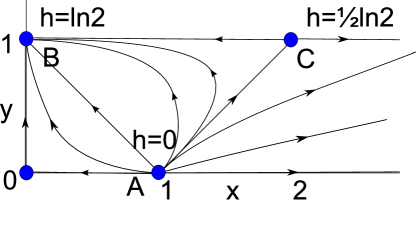
Figure 2: Decimation RG flow for the spin-1 model spo with the values of entropy per lattice site $h$ at some fixed points.

The resulting quite interesting RG flow diagram obtained in spo is shown schematically in Fig. 2. Its main features are four fixed points and a critical line AC. Since this flow arises from the decimation transformation our general arguments require that the entropy per site $h(x,y)$ should increase along the flow. Though the model can be solved exactly (see spo for details) it is easy to evaluate the entropy at the fixed points without much computations.

The point A corresponds to fully ordered state (actually there are three such states with all $s_{i}$ either $+1$, or $-1$, or 0) hence $h_{A}=H/N=0$ at $N\rightarrow\infty$ with only subextensive contribution to $H$. The same is true also for the point $x=y=0$ with two ordered states. The point B is similar to a high temperature fixed point of the Ising model, with uncorrelated $s_{i}=\pm 1$ and no zero spins, hence $h_{B}=\ln 2$.

The most interesting case is the critical point C at $x=2,y=1$. It corresponds to $K_{1}=0$ while $K_{3}-K_{2}=\ln 2$. In this case there exist the lowest energy state with all $s_{i}=0$ and zero energy. For periodic boundary condition all configurations with some finite fraction of spins changed to $\pm 1$ have infinite energy at $K_{3}\rightarrow\infty$ while states with all $s_{i}=\pm 1$ are gapped with $\Delta E=N\ln 2$. But there are $2^{N}=\exp(N\ln 2)$ such states and their statistical weight exactly compensates the Boltzmann factor $\exp(-\Delta E)$ which results in the partition function $Z=2$ and mean energy $\langle S\rangle=\Delta E/2$. Therefore at C we effectively have two equally probable states with highly degenerate disordered excited one and the resulting entropy $h_{C}=(\langle S\rangle+\ln Z)/N\rightarrow(1/2)\ln 2$ at $N\rightarrow\infty$.

The values of entropies are shown in Fig. 2 near the corresponding fixed points. We see now that the entropy per site can in fact be used to understand the ordering of the fixed points along the flow since $h$ monotonically grows when we pass from A to C and finally to B.

Certainly this is not the only way to classify these fixed points. In fact we can use also the degeneracy $q$ of the largest eigenvalue of the transfer matrix $T$ (actually the degeneracy of the ground state of the corresponding quantum Hamiltonian $\hat{H}$, defined by $\hat{T}=\exp(-\hat{H})$). In 1D $q$ plays, in a sense, the same role as the central charge $c$ in two dimensions, because $q$ always decreases under renormalization (this also resembles the $g$-theorem g for 1D quantum systems). The global decrease of $q$ in 1D spin system with nearest-neighbor interactions when

$$S=\sum_{i}V(s_{i},s_{i+1})$$ (36)

is rather trivial and follows directly from the decimation RG transformation written as a transfer matrix mapping

$$T\rightarrow T^{\prime}=T^{2},\qquad T_{s,s^{\prime}}=\exp(-V(s,s^{\prime}))$$ (37)

where for spin with $n$ possible values $T$ is a nonnegative $n\times n$ matrix. Eigenvalues of $T$ transform as $\lambda_{i}\rightarrow\lambda_{i}^{\prime}=\lambda_{i}^{2}$ so that the degeneracy once reduced will never return back. For strictly positive $T$ Frobenius theorem requires $q=1$, but when some couplings turn to infinity, as we have seen above for the spin-1 model, some entries in $T$ may vanish and $q$ may differ from unity. For the spin-1 model all these eigenvalues were calculated in Ref. spo and $q=3$ for point A, $q=2$ for C (also for the point at the origin) and $q=1$ for point B in Fig. 2.

For these models it is possible also to evaluate the excess entropy at the fixed points. Fixed points for decimation are defined by

$$T^{\prime}=T^{2}=\lambda T$$ (38)

where $\lambda$ is some positive number (multiplication of $T$ by a constant does not change the physics) and it can be easily shown that in these cases $T$ may have $q\leq n$ eigenvalues $\lambda$ while other eigenvalues are zeros. Then for the periodic boundary condition

$$Z={\rm tr}(T^{N})=q\lambda^{N},\quad\Rightarrow\quad\ln Z=N\ln\lambda+\ln q$$ (39)

and since $\langle S\rangle\sim N$ entropy at fixed points has the form $Nh+C$ with $C=\ln q$. In this case the subextensive part in $H$ coincides with that in $\ln Z$ and this number monotonically decreases when we pass from one fixed point to another along the RG flow (this is somewhat similar in spirit to the recently proposed $F$-theorem for field theories in odd dimensions Ftheor ). Unfortunately, for periodic boundary conditions $C$ equals $\ln q$ also away from fixed points (at $N\rightarrow\infty$) and it is discontinuous, because $q$ changes abruptly, while excess entropy for a finite block in an infinite chain, which is related to mutual information of two halves and is expected to be continuous and monotonic along the RG flow, is much harder to evaluate at $s\geq 1$ and in general is no more related to $q$ in a simple way even at fixed points.

IV.3 Decimation in two dimensions.

Consider now a two-dimensional classical spin system, with spins placed on sites of a square lattice. Various spin interactions, including e.g. nearest-neighbor, second-nearest-neighbor and similar interactions, are parameterized by a set of coupling constants ${\bf K}=(K_{1},K_{2},\ldots)$. To define a “checkerboard” decimation transformation we first divide the lattice into two interpenetrating square sub-lattices and then sum over all spins on one sublattice KH (see Fig. 1b). Just as in one dimension we obtain then a new spin system again on a square lattice (with the lattice spacing $\sqrt{2}$ times larger) but with a new energy $S^{\prime}$ with couplings ${\bf K}^{\prime}$. This is the first step of the RG transformation, which is then repeated further.

Since two sub-lattices are identical the mutual information between them is again given by the Eq. (29), i.e.

$$I/N=h({\bf K}^{\prime})-h({\bf K})\geq 0$$ (40)

for a large lattice with $N$ sites, where $h({\bf K})$ is the entropy per site. Hence we conclude that in this case the entropy per site should also increase in the course of the RG transformation and the RG flow is irreversible.

The entropy growth in two dimensions may seem a rather counterintuitive result, since in systems with phase transition one may naïvely expect that at low temperatures (below the transition) the RG transformation should lead us deeply into the ordered phase with $h({\bf K}^{\prime})$ decreasing to zero. But for the decimation this intuition obviously doesn’t work, since in this case the average spin remains unchanged so that the spontaneous magnetization is constant along the RG flow.

For better understanding of why the entropy per site can grow under renormalization at low temperatures let us now consider the ferromagnetic Ising model with $S=-K_{1}\sum_{{\rm nn}}s_{i}s_{j}$, where the sum is over nearest-neighbors and $s_{i}=\pm 1$. After the first step of the RG we have (up to an unimportant constant) W

$$S^{\prime}=-K_{1}^{\prime}\sum_{{\rm nn}}s_{i}s_{j}-K_{2}^{\prime}\sum_{{\rm nnn}}s_{i}s_{j}-K_{3}^{\prime}\sum_{{\rm P}}\prod_{i=1}^{4}s_{i},$$ (41)

where the second term is the next-nearest-neighbor interaction and the last one is the four spin interaction ($s_{i}$, $i=1\ldots 4$ are spins on the corners of a plaquette) with the sum over all plaquettes. The new coupling constants are known to be

$$K_{1}^{\prime}=2K_{2}^{\prime}=\frac{1}{4}\ln(\cosh 4K_{1}),$$ (42)

$$K_{3}^{\prime}=\frac{1}{8}\ln(\cosh 4K_{1})-\frac{1}{2}\ln(\cosh 2K_{1})$$ (43)

We see now that $K_{1}^{\prime}>0$ (though $K_{1}^{\prime}<K_{1}$), the next-nearest-neighbor interaction is also ferromagnetic, $K_{2}^{\prime}>0$, but $K_{3}^{\prime}<0$, i.e. the four-spin interaction tries to decrease the ferromagnetic order.

Next, we estimate the entropy at low temperatures. At $K_{1}\rightarrow\infty$ all spins point in one direction and the entropy is different from zero only due to rare spin flips. The partition function may be represented as a low temperature expansion

$$Z=2{\rm e}^{-NE_{0}}\left(1+N\exp(-\Delta E({\bf K}))+\ldots\right),$$ (44)

where $NE_{0}$ is the energy of all spins aligned and the energy needed to reverse one spin is $\Delta E=8K_{1}$ in original system since after the reversal four links have “wrong” alignment of adjacent spins. Hence at low temperatures the entropy per site is

$$h\simeq 8K_{1}\exp(-8K_{1})+\ldots$$ (45)

After the decimation the system is still ferromagnetic but the energy of spin reversal is now $\Delta E^{\prime}=8K_{1}^{\prime}+8K_{2}^{\prime}+8K_{3}^{\prime}$ or

$$\Delta E^{\prime}=4\left(\ln(\cosh 4K_{1})-\ln(\cosh 2K_{1})\right)\simeq 8K_{1}-4{\rm e}^{-4K_{1}}$$ (46)

at large $K_{1}$. Hence the new excitation energy is smaller than $\Delta E$ and it becomes easier to reverse a spin. However, since the difference is exponentially small one has to include also the next term in $h({\bf K})$ due to pairs of reversed spins $24K_{1}\exp(-12K_{1})$ (the corresponding term in $h({\bf K}^{\prime})$ can be easily evaluated as $\sim\exp(-16K_{1})$ and is unimportant). But even with this contribution taken into account the entropy per site after the decimation $h({\bf K}^{\prime})\simeq\Delta E^{\prime}\exp(-\Delta E^{\prime})$ is larger,

$$h({\bf K}^{\prime})-h({\bf K})\simeq 8K_{1}{\rm e}^{-12K_{1}}>0.$$ (47)

Thus, it is possible to check at least for the first iteration at low temperatures that indeed the entropy per site grows after the decimation. Physically the result (47) for the mutual information or $I\sim N\exp(-12K_{1})$ is due to the reversed pairs of adjacent spins in the original lattice. Only through these pairs the two sub-lattices have non-trivial information about each other at $K_{1}\rightarrow\infty$ (there should be also a term $\ln 2$ in $I$ since the orientations of the overall magnetization in sub-lattices are correlated, but we are interested only in terms $\sim N$ in the mutual information).

Now it is possible to explain, what this increase in entropy at low temperatures actually means. Since the average magnetization conserves along the decimation RG flow, the average number of reversed spins per unit volume remains the same, but now more of them are isolated ones (with less energy cost of reversal) and the number of reversed close pairs or larger clusters is relatively smaller than in the initial system. Surely this picture may also be interpreted as a decrease in the correlation length for spin fluctuations.

Unfortunately the next iteration of the decimation cannot be performed exactly and is known to lead to non-Gibbsian measures at low temperatures nG , so that it is not possible to describe renormalization as a flow in usual space of couplings. Still there should be a flow of probability measures, probably with limiting points corresponding to product measures describing independent spins with fixed total magnetization.

IV.4 Kadanoff block-spin transformation

Consider now a classical lattice system of Ising spins $s_{i}$ with the action $S_{0}[s]$ and first divide the lattice into a set of nonoverlapping identical blocks with, say, $k$ adjacent spins in each block $B_{j}$, assuming that blocks form a lattice, similar to the original one (see Fig. 3 for an example). Then, following Kadanoff prescription K associate a new spin variable $t_{j}$ with $j$-th block and define the RG transformation $S_{0}[s]\rightarrow S^{\prime}[t]$ according to

$$\exp(S^{\prime}[t])=\sum_{s}T(t,s)\exp(-S_{0}[s])$$ (48)

with $T(t,s)>0$ obeying the condition

$$\sum_{t}T(t,s)=1$$ (49)

which guarantees that the partition function $Z$ is the same for both $s$ and $t$ variables.

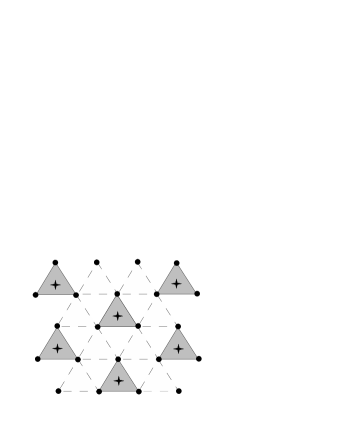
Figure 3: Block-spin transformation on a triangular lattice for $k=3$. Blocks $B_{j}$ are shaded, spins $s_{i}$ are located at black sites while block variables $t_{j}$ may be placed in the centers of blocks.

This transformation is of the general type of Eq. (2) but now all $s_{i}$ are “fast” variables and $t_{j}$ are “slow” ones. Hence the total “action” $S[t,s]=-\ln T(t,s)+S_{0}[s]$ now defines the joint probability for initial and “renormalized” spins. The entropy $H$ now is not equal to the physical entropy $H_{0}$ of the initial spin system but is given by

$$H(t,s)=\langle S\rangle_{S}+\ln Z=\langle S_{0}\rangle_{S_{0}}-\langle\ln T\rangle_{S}+\ln Z=$$ (50)

$$=H_{0}-\langle\ln T\rangle_{S},$$

where we have used the condition (49) in the calculation of $\langle S_{0}\rangle_{S}$.

The most popular form of $T(t,s)$ is

$$T(t,s)=\prod_{j}\frac{\exp(pt_{j}S_{j})}{2\cosh(pS_{j})},$$ (51)

where $p$ is a free parameter and

$$S_{j}=\sum_{i\in B_{j}}s_{i}$$ (52)

is the sum of initial spins in the block $B_{j}$. Note that $pt_{j}$ enters in the partition function as a spatially varying magnetic field constant over a block. Hence at $p\rightarrow\infty$ all block spins $S_{j}$ will be aligned strictly along $t_{j}$. Now making use of the identity $\langle t_{j}\rangle_{S}=\langle\tanh(pS_{j})\rangle_{S_{0}}$ we easily obtain

$$-\langle\ln T\rangle_{S}=\sum_{j}\langle f(pS_{j})\rangle_{S_{0}},\,$$ (53)

$$f(x)=-x\tanh x+\ln(2\cosh x),$$

where the sum is over all blocks. Next, we can easily sum $\exp(-S[t,s])$ over $t$ because of the identity (49) to obtain $\tilde{S}^{\prime}[s]=S_{0}[s]$ and hence

$$H(s)=H_{0}$$ (54)

Now we can use the definition of the mutual information (III) and Eqs. (50), (54) to derive the final expression

$$I=H(t)+H(s)-H(t,s)=H(t)-\sum_{j}\langle f(pS_{j})\rangle_{S_{0}}$$ (55)

Note that $H_{0}$ cancels away from the resulting expression for the mutual information. Next we introduce the entropy per lattice site for renormalized spins according to $H(t)=(N/k)h({\bf K}^{\prime})$ and instead of $I=N(h({\bf K}^{\prime})-h({\bf K}))$ which was valid for decimation, we have at large $N$ quite a different expression

$$I=\frac{N}{k}[h({\bf K}^{\prime})-\langle f(p\sum_{i}s_{i})\rangle_{0}]\geq 0,$$ (56)

where the sum of spins $s_{i}$ is over one block, $k$ is the number of spins in a block and the average is over the initial configurations with the weight $\exp(-S_{0}[s])$. The second term in Eq. (56) looks like the entropy of the total spin of a block at temperature $1/p$ averaged over different values of its magnitude.

Thus the entropy after the renormalization $h({\bf K}^{\prime})$ is always bounded from below, provided the second term in Eq. (56) is nonzero. This is due to the noise induced by the renormalization at finite $p$.

The most interesting case however corresponds to $p\rightarrow\infty$ which is known to lead to the so called majority-rule renormalization MR . This means that we define $t_{j}$ as $\pm 1$ depending on the sign of the total block spin $S_{j}$. We assume also that $k$ is odd to avoid ambiguities. Then $S_{j}\neq 0$ and from Eq. (53) it follows that $f(pS_{j})\rightarrow 0$ at $p\rightarrow\infty$ leading to

$$I=H^{\prime}=\frac{N}{k}h({\bf K}^{\prime}),\qquad p\rightarrow\infty,\qquad k-{\rm odd}.$$ (57)

This result is rather obvious however, because from Eq. (III) we have $I=H^{\prime}-H(t|s)$ but for majority-rule RG the initial configuration of spins $s_{i}$ completely determines that of renormalized spins $t_{j}$ so that $H(t|s)=0$ (there is no noise in the transmission channel) and hence their mutual information coincides with the final entropy $I=H^{\prime}$. Therefore in this case the positivity of mutual information gives nothing new and $h({\bf K}^{\prime})$ can be either greater or smaller than $h({\bf K})$. Contrary to decimation now $I\geq 0$ does not prohibit fixed points and the entropy per site can even go to zero along the RG flow.

IV.5 One dimensional free field theory

Now we proceed to quantum field theory, using ordinary quantum mechanics as the simplest example. Consider a quantum particle of mass $m$, moving along a line in a harmonic potential well with a frequency $\omega$. Its partition function at a temperature $T$ is given by a path integral, which in a lattice regularization, when the imaginary time interval $[0,\beta]$ ($\beta=1/T$) is divided into $N$ intervals of length $\epsilon$, has the form

$$Z=\left(\frac{m}{2\pi\epsilon}\right)^{N/2}\int\exp(-S)\prod_{i=1}^{N}dx_{i},$$

$$S=\sum_{i}\frac{m}{2}\frac{(x_{i+1}-x_{i})^{2}}{\epsilon}+\epsilon\sum_{i}\frac{m\omega^{2}}{2}x_{i}^{2},$$ (58)

with $N=\beta/\epsilon$. Shannon entropy, as mentioned above, equals

$$H=\langle S\rangle+\ln Z,$$ (59)

where brackets mean the average with weight $\exp(-S)$. $H$ coincides with the entropy of the statistical system of variables $x_{i}$ placed on sites of a one-dimensional lattice of length $\beta$ with nearest-neighbor interaction and periodic boundary condition. This system is actually the one-dimensional Gaussian model near its critical point $\omega=0$ GA .

However, at $\epsilon\rightarrow 0$ this model is actually (0+1) Euclidean free field theory and its thermodynamic entropy is given by a different formula

$$H_{T}=(E-F)/T=E\beta+\ln Z$$ (60)

where $E$ is the mean energy of the particle and $F=-T\ln Z$ is its free energy. Let us now briefly discuss the connection between these two entropies.

The mean velocity squared $\langle\dot{x}^{2}\rangle$ which enters in $\langle S\rangle$ diverges as $\epsilon\rightarrow 0$ F and its direct evaluation is not so easy, but the average action can be evaluated simply by differentiating $Z$ with respect to mass

$$m\frac{\partial Z}{\partial m}=\frac{N}{2}Z-\langle S\rangle Z,$$ (61)

where the first term in the r.h.s. comes from the differentiation of $m$ in the integration measure. But for the harmonic oscillator $Z$ does not depend on mass, and therefore $\langle S\rangle=N/2$. In the continuum limit

$$\ln Z=-\ln(2\sinh(\omega\beta/2)),$$ (62)

and at a given $\omega$ we have the following asymptotics for the entropies at $\beta\rightarrow\infty$

$$H=\frac{\beta}{2}\left(\frac{1}{\epsilon}-\omega\right)+{\rm e}^{-\omega\beta}+\ldots$$ (63)

$$H_{T}=\omega\beta{\rm e}^{-\omega\beta}+\ldots$$ (64)

We see that the leading “bulk” term in $H$ is divergent in the continuum limit $\epsilon\rightarrow 0$ and $H_{T}$ resembles, in a sense, the finite size correction in $H$.

The different behavior of $H$ and $H_{T}$ comes from the fact that $H_{T}$ describes the information related to energy levels occupation and hence tends to zero at zero temperature when the system is in its ground state, while $H$ describes fluctuations of “paths” in configuration space which obviously grow as $\beta\rightarrow\infty$.

The entropy per lattice site here is

$$h=\frac{1}{2}-\frac{\epsilon\omega}{2}+\ldots$$ (65)

at $\epsilon\rightarrow 0$. It may seem strange that $h$ decreases with correlation length $\xi=(\omega\epsilon)^{-1}$, because for the model in question we may also apply the decimation transformation, similar to that in the Ising model, integrating away $x_{i}$’s on alternating sites (see e.g. Kb ) and our general result states that in this case $h$ should increase along the RG flow. Under such a decimation $\xi\rightarrow\xi/2$ and $h$ from Eq. (65) does not behave in the required way.

The solution to this apparent contradiction is rather simple. Note first that summation over variables $x$ is defined now as

$$\sum_{x}(\ldots)=\int\prod_{i}\left(\sqrt{\frac{m}{2\pi\epsilon}}dx_{i}\right)(\ldots)$$ (66)

and the integration measure itself depends on mass and on lattice spacing. This integration measure is fine-tuned to the action so that $Z$ has a well defined correct continuum limit (62). But after the RG transformation this fine-tuning is destroyed. The effective action $S^{\prime}$ now contains renormalized mass $m^{\prime}$, frequency $\omega^{\prime}$ and a new lattice spacing $2\epsilon$, but the measure (66) remains the same. This means that in this case the entropy after renormalization is no longer given by the same formula (63) as before.

We may transform the measure to the correct form but this leads to an additional factor $(2m/m^{\prime})^{N/4}$ in $Z$, since the lattice now has $N/2$ sites. This additional factor does not affect the mean action $\langle S^{\prime}\rangle$ but certainly change the $\ln Z$ part of the entropy. Simple Gaussian integration like that in Ref. Kb shows that $m^{\prime}\simeq m$ up to the terms of order $\epsilon^{2}$ at $\epsilon\rightarrow 0$ and the additional factor is simply $2^{N/4}$. Then the new entropy per site equals

$$h^{\prime}=\frac{1}{2}+\frac{1}{2}\ln 2+\ldots,$$ (67)

at $\epsilon\rightarrow 0$. This quantity is larger than $h\simeq 1/2$ and the mutual information $I$ of two sublattices is given by

$$I=N(h^{\prime}-h)=\frac{N}{2}\ln 2$$ (68)

at $\epsilon\rightarrow 0$. Note also that the total entropy is reduced after the decimation, because the information loss $\delta I=H-H^{\prime}=N(1-\ln 2)/4$ is positive.

Let us now analyze this system more carefully. After the decimation is repeated many times we get away from the continuum limit because the lattice spacing grows. In this region it is more convenient to rewrite the renormalized action in the form

$$S=\sum_{i}Kx_{i}x_{i+1}+\frac{b}{2}\sum_{i}x_{i}^{2},$$ (69)

where $K$, $b$ are new running coupling constants with the initial values $K_{0}=m/\epsilon$, $b_{0}=2m/\epsilon+\epsilon m\omega^{2}$. The entropy per lattice site for this action can be derived from the exact solution of the Gaussian model GA

$$h = \frac{1}{2}+\frac{1}{2}\ln\left(\frac{K_{0}}{b}\right)-\frac{1}{2}\int_{0}^{2\pi}\frac{dt}{2\pi}\ln\left(1-2\frac{K}{b}\cos t\right)=$$ (70)

$$=\frac{1}{2}+\frac{1}{2}\ln\left(z\frac{K_{0}}{K}\right)-\frac{1}{2}\ln{\frac{1+\sqrt{1-4z^{2}}}{2}},\quad z=\frac{K}{b},$$

where $K_{0}=m/\epsilon$ comes from the integration measure in Eq. (IV.5). Note that while all correlations depend only on $z=K/b$, the entropy depends on both $K$ and $b$ because the integration measure contains the unrenormalized coupling $K_{0}$. Decimation acts as

$$K^{\prime}=\frac{K^{2}}{b},\quad b^{\prime}=b-2\frac{K^{2}}{b},$$ (71)

or $z^{\prime}=z^{2}/(1-2z^{2})$. This RG equation has a fixed point $z^{*}=1/2$ which corresponds to $\omega=0$ and under renormalization $z$ flows to $z=0$. Close to the fixed point $z=1/2$ one can define a continuous theory by choosing $K\simeq b/2\simeq m/\epsilon$ and $b-2K=\epsilon m\omega^{2}$ with $\epsilon\rightarrow 0$ and RG equations turn into $K^{\prime}\simeq K/2$, $b^{\prime}\simeq b/2$.

It is now easy to verify that in the vicinity of $z=1/2$ the initial value of the entropy is $h=1/2$ and that it indeed acquires an additional $(1/2)\ln 2$ contribution at each decimation step provided we are still close to the fixed point. Note that $h$ grows even for $z=1/2$ because in the two dimensional space of $K$ and $b$ there is no critical fixed point and the point $z=1/2$ corresponds to a line $K=b/2$ with the RG flow along it. After many decimations $z\rightarrow 0$, i.e. $K$ decreases much faster than $b$ and the entropy starts to behave as

$$h\simeq\frac{1}{2}\ln\left(\frac{K_{0}}{b}\right),\quad K\ll b\ll K_{0}$$ (72)

with logarithmic accuracy. Since $K\rightarrow 0$ means the loss of correlations between $x$’s on different sites, this expression for the entropy $h$ is in fact the entropy production rate for the Gaussian white noise $h\sim\ln\sigma$ with dispersion $\sigma^{2}\sim 1/b$, well known in the information theory.

V Conclusion

In this paper we have tried to understand what limitations on the RG flow may follow from the information theory, because Wilsonian RG transformation, when some fast variables are integrated out, is obviously related to the information loss. This transformation is similar in a sense to a signal transmission through a noisy channel, the fast variables being the input, while the slow ones play the role of the output available to a receiver. The information loss is defined here as an average conditional entropy of the eliminated fast variables when the remaining slow variables are fixed. From the nonnegativity of this quantity (which holds at least for systems with discrete variables, like e.g. classical spins) it follows immediately that the informational entropy $H$ of the system cannot increase under renormalization.

Unfortunately this result is not very interesting, and does not lead to the irreversibility of the RG flow, because it applies to the total extensive entropy, proportional to the size of the system, which effectively shrinks after renormalization. This shrinking is evident for real space RG schemes, where some lattice sites are eliminated and the system size is smaller if measured in new lattice constant, but equally applies to momentum space Wilsonian renormalization due to final rescaling of momenta.

Only if $H$ possesses some volume independent additive part $C$, then this part, if it also decreases under renormalization, may provide the required Lyapunov function, that depends only on couplings. Physically its decrease may be attributed to a loss of information about massless modes, but this does not follow directly from that of $H$ and should be deduced independently. Then, to be monotonous $C$ must have also some independent definition. For 1D Ising model this quantity is just the subextensive excess entropy and we explicitly check its monotonicity under RG transformation. This behavior for a finite block of spins in an infinite chain follows directly from information theory, because excess entropy in this case is just the mutual information of two halves of the system FC , which decreases under coarse graining.

Note also that for 1D systems with periodic boundary conditions the excess entropy is $\ln q$ where $q$ is the degeneracy of the largest eigenvalue of the transfer matrix which always decreases along the RG flow. This is somewhat similar to what is known for critical 2D systems defined on a long cylinder of size $L_{x}\times L_{y}$ with, say, $L_{y}\rightarrow\infty$ and periodic boundary condition in the $x$ direction. In this case the first finite size correction in the expansion of entropy in $1/L_{x}$ is $\sim c(L_{y}/L_{x}$) fs , where $c$ is the central charge. Therefore the subextensive part $C$ in entropy in 2D should decrease as a consequence of the $c$-theorem. However in both these examples the subleading term in entropy is discontinuous and does not directly lead to a proper Lyapunov function.

This means that the extraction of the required part from the entropy of finite size system is somewhat ambiguous and depends on the boundary condition. One may suggest, however, that in general there might exist some size-independent information-based quantity defined on the whole space of couplings (maybe some kind of relative entropy or higher order mutual information ho ) that is monotonic along the flow and at fixed points coincides with some kind of excess entropy, but this point is not clear.

The main aim of the present paper was, however, apart from demonstrating some examples of informational approach, to introduce a different quantity, namely the mutual information of fast and slow variables $I$, which shows how much information about the eliminated variables is still stored in the renormalized effective action. This quantity does not suffer from the “shrinking size” trouble and is less sensitive to the overall decrease in the number of degrees of freedom, though it is generally more difficult to evaluate.

There exist however some real space decimation transformations for which this mutual information can be easily calculated. This happens e.g. if the original lattice may be decomposed in two identical sublattices and RG transformation eliminates spins on one sublattice. Then the nonnegativity of $I$ results in the increase of entropy per lattice cite and RG flow resembles a relaxation to equilibrium. This result does not depend on interactions and may be true also for a larger set of models. What is actually needed is that the RG transformation must be represented as a product of such decimations.

The approach to irreversibility based on the mutual information is different from those trying to generalize Zamolodchikov’s $c$-theorem and possibly may provide some additional information about the RG flows. It may appear interesting also to apply the present approach to the momentum space renormalization in field theory or to study more complicated correlations along the flow and some higher-order mutual information.

I am very grateful to A.C.D. van Enter, J. Gaite, V. Losyakov, A. Marshakov, A. Morozov for valuable discussions and comments, and to L. Shchur for some useful advices. The work was supported in part by RFBR grants 09-02-00886, 10-02-00509, RFBR-Ukraine 09-01-90493 and by Federal Agency for Science and Innovations of Russian Federation under contract 14.740.11.0081.

References

- (1) K.G. Wilson and J. Kogut, Phys. Rep. 12 75 (1974); K.G. Wilson, Rev. Mod. Phys. 47 773 (1975)
- (2) C. Bagnuls and C Bervillier, Phys. Rep. 348 91 (2001); B. Delamotte, arXiv:cond-mat/0702365
- (3) A.B. Zamolodchikov, Pis’ma Zh. Eksp. Teor. Fiz. 43 565 (1986) [JETP Lett. 43 730 (1986)]
- (4) J.L. Cardy, Phys. Lett. B215 749 (1988); I. Jack and H. Osborn, Nucl. Phys. B343 647 (1990); A. Cappelli, D. Friedan and J.I. Latorre, Nucl. Phys. B352 616 (1991); A.H. Castro Neto and E. Fradkin, Nucl. Phys. B400 525 (1993); S. Forte and J.I. Latorre, Nucl. Phys. B535 709 (1998); T. Appelquist, A.G. Cohen and M. Schmaltz, Phys. Rev. D 60 045003 (1999); A. Cappelli, G. D’Appollonio, R. Guida and N. Magnoli, arXiv:hep-th/0009119; D. Anselmi, Acta Phys. Slov. 52 573 (2002); E. Barnes, K.A. Intriligator, B. Wecht and J. Wright, Nucl. Phys. B702, 131 (2004)
- (5) D.L. Jafferis, I.R. Klebanov, S.S. Pufu and B.R. Safdi, arXiv:1103.1181; A. Amariti and M. Siani, arXiv:1105.3979; I.R. Klebanov, S.S. Pufu and B.R. Safdi, arXiv:1105.4598.
- (6) A. Morozov and A.J. Niemi, Nucl. Phys. B666 311 (2003)
- (7) S.R. McKay, A.N. Berker and S. Kirkpatrick, Phys. Rev, Lett. 48 767 (1982); N.M. Švrakić, J. Kertész and W. Selke, J. Phys. A 15 L427 (1982); B. Derrida, J.-P. Eckmann and A. Erzan, J. Phys. A 16 893 (1983)
- (8) P.H. Damgaard and G. Thorleifsson, Phys. Rev. A 44 2738 (1991); P.H. Damgaard, Int. J. of Mod. Phys. A 7 6933 (1992)
- (9) B.P. Dolan, Phys. Rev. E 52 4512 (1995)
- (10) S.D. Głazek and K.G. Wilson, Phys. Rev. Lett. 89 230401 (2002); E. Braaten and H.-W. Hammer, Phys. Rev. Lett. 91 102002 (2003); S. D. Głazek and K.G. Wilson, arXiv:cond-mat/0303297
- (11) J. Gaite and D. O’Connor, Phys. Rev. D 54 5163 (1996)
- (12) J. Gaite, Phys. Rev. Lett. 81 3587 (1998); J. Gaite, Phys. Rev. D 61 045006 (2000); Phys. Rev. D 62 125023 (2000)
- (13) P.L. Ferrari and J.L. Lebowitz, J. Phys. A 36 5719 (2003)
- (14) A. Robledo, J. Stat. Phys. 100 475 (2000)
- (15) J.P. Crutchfield and D.P. Feldman, Phys. Rev. E 52 1239R (1997); D.P. Feldman and J.P. Crutchfield, Phys. Rev. E 67 92 (2003)
- (16) T.M. Cover and J.A. Thomas, Elements of Information Theory, 2nd ed. (Wiley, Hoboken, NY) 2006
- (17) S. Krinsky and D. Furman, Phys. Rev. Lett. 32 731 (1974); Phys. Rev. B 11 2602 (1975)
- (18) L.P. Kadanoff and A. Houghton, Phys. Rev. B 11 377 (1975)
- (19) L. Sneddon and M.N. Barber, J. Phys. C:Solid State Phys. 10 2563 (1977)
- (20) I. Affleck and A.W.W. Ludwig, Phys. Rev. Lett. 67 161 (1991); D. Friedan and A. Konechny, Phys. Rev. Lett. 93 030402 (2004)
- (21) A.C.D. van Enter, R. Fernández and A.D. Sokal, J. Stat. Phys. 72 879 (1993); A.C.D. van Enter, F. Redig and E. Verbitskiy, arXiv:0804.4060
- (22) L.P. Kadanoff, Rev. Mod. Phys. 49 267 (1977)
- (23) Th. Niemeijer and J.M.J. van Leeuwen, in Phase Transition and Critical Phenomena, Vol. 6, eds. C. Domb and M.S. Green (Academic Press, New York, 1976)
- (24) T.H. Berlin and M. Kac, Phys. Rev. Lett. 86 821 (1952)
- (25) R.P. Feynman and A.R. Hibbs, Quantum Mechanics and Path Integrals (McGraw Hill Inc., New York, 1965)
- (26) L.P. Kadanoff, Statistical Physics. Statics, Dynamics and Renormalization (World Scientific, Singapore, 2000)
- (27) H. Matsuda, Phys. Rev. E 62 3096 (2000)
- (28) H.W.J. Blöte, J.L. Cardy and M.P. Nightingale, Phys. Rev. Lett. 56 742 (1986); I Affleck, Phys. Rev. Lett. 56 746 (1986)