The Electron Propagator in External Electromagnetic Fields in Lower Dimensions

Abstract

We study the electron propagator in quantum electrodynamics in lower dimensions. In the case of free electrons, it is well known that the propagator in momentum space takes the simple form $S_{F}(p)=1/(\gamma\cdot p-m)$. In the presence of external electromagnetic fields, electron asymptotic states are no longer plane-waves, and hence the propagator in the basis of momentum eigenstates has a more intricate form. Nevertheless, in the basis of the eigenfunctions of the operator $\left(\gamma\cdot\Pi\right)^{2}$, where $\Pi_{\mu}$ is the canonical momentum operator, it acquires the free form $S_{F}(p)=1/(\gamma\cdot\overline{p}-m)$ where $\overline{p}_{\mu}$ depends on the dynamical quantum numbers. We construct the electron propagator in the basis of the $\left(\gamma\cdot\Pi\right)^{2}$ eigenfunctions. In the (2+1)-dimensional case, we obtain it in an irreducible representation of the Clifford algebra incorporating to all orders the effects of a magnetic field of arbitrary spatial shape pointing perpendicularly to the plane of motion of the electrons. Such an exercise is of relevance in graphene in the massless limit. The specific examples considered include the uniform magnetic field and the exponentially damped static magnetic field. We further consider the electron propagator for the massive Schwinger model incorporating the effects of a constant electric field to all orders within this framework.

I Introduction

A powerful technique to solve wave equations in quantum theory is the Green’s function method. The evolution of the wave functions is encoded in the propagators, which in plain words are the inverses of the differential wave operators. For free particles, which are described by plane-waves, these propagators acquire simple diagonal forms in momentum space due to the isotropy of the space. However, when the isotropy is lost, particles cease to be described as plane-waves and their corresponding propagators have more intricate forms in the basis of momentum eigenstates, sometimes at the point of being intractable for actual calculations. An example of such systems is a gas of electrons subject to an intense magnetic field in a fixed direction. The non-relativistic quantum problem for this system, known as the Landau problem, Landau reveals interesting features of the dynamics of electrons in external magnetic fields. On one hand, the Lorentz force lacks of component along the direction of the field. This makes a clear separation between the parallel (free) and transverse (dynamical) components of the trajectories of the electrons with respect to the field lines. On the other hand, in the transverse plane, the trajectories are confined around the field lines. In such a case, the energy levels, called Landau levels, develop a discrete spectrum. These features combined translate into a rather intricate form of the electron propagator brasileiros as compared with its free counterpart. For relativistic electrons, the problem does not get any simpler. Yet, the task of unveiling these propagators for systems just as complicated is worthwhile.

There have been a number of strategies developed in the past to derive the propagator for relativistic electrons in background electromagnetic fields, perhaps the best known being the Fock-Schwinger “proper time” method, Fock ; Schwinger which was originally developed in relativistic quantum field theory (see Ref. [5] for a brief discussion of the method), but that has been applied to a number of problems in ordinary non-relativistic quantum mechanics. brasileiros ; otros However, there have been interesting alternatives to the Fock-Schwinger method to incorporate the effects of the background fields into the propagators, like the second quantization of solutions to the Dirac equation in the background fields, Kaushik path integral methods, path and the Ritus eigenfunction method. Ritus In this article, we derive the massive electron propagator in background electromagnetic fields in lower space-time dimensions through the later method, which is based upon the diagonalization of the Dirac operator on the basis of the eigenfunctions of the operator $\left(\gamma\cdot\Pi\right)^{2}$, with $\Pi_{\mu}$ being the canonical momentum operator.

We begin this article by considering the $d$-dimensional free electron propagator in Sect. II. The details of the Ritus method are presented in Sect. III. For the sake of simplicity, we present the study of the electron propagator in (2+1)-dimensional QED, where a third spatial dimension is suppressed. This is not a mere theoretical simplification, and we explain ourselves: back in time, some twenty years ago, Semenoff it was shown that the low-energy effective theory of graphene in a tight-binding approach is the theory of two species of massless Dirac electrons in a (2+1)-dimensional Minkowski space-time, each on a different irreducible representation of the Clifford algebra. The isolation of graphene samples Novoselov in 2004 and 2005, has given rise to the new paradigm of relativistic condensed matter, graphene bringing a new boost, both theoretical and experimental, to the matching of common interests of the condensed matter and high energy physics communities. Thus, the massless limit of our findings is of direct relevance in this subject. planarqed We assume the electrons moving in a magnetic field alone pointing perpendicularly to their plane of motion. We first develop the general case and then, in Sect. IV we present a couple of examples: the motion of electrons in a uniform magnetic field, which is a canonical example to present the Ritus method, Khalilov and the case of a static magnetic field which decays exponentially along the $x$-axis. The effects of such a magnetic field to all orders can hardly be considered with other approaches, but it can be straightforwardly studied within the Ritus method.

Electric field configurations can also be studied in this framework. With this goal in mind, in Sect. V we analyze the electron propagator in a constant electric field in the massive Schwinger model Schwinger , that is, quantum electrodynamics in (1+1)-dimensions. The Schwinger model exhibits spontaneous symmetry breaking of the $U(1)$ symmetry, as well as confinement of electrons, thus is a favorite toy model to study some aspects of quantum chromodynamics. These properties can be studied from the electron propagator, which acquires a free form when expressed in the basis of the eigenfunctions of the operator $\left(\gamma\cdot\Pi\right)^{2}$. We settle the basis for such studies in this article. In Sect. VI we present a discussion and final remarks. At the end, we propose a project for the interested reader, in which the Ritus method has to be applied in order to obtain the electron propagator in a different situation than the considered here.

II Free Dirac Propagator

We start our discussion from the equation of motion for free electrons, namely, the Dirac equation fn1

$$(i\gamma\cdot\partial-m)\psi(x)=0,$$ (1)

where the $\gamma^{\mu}$-matrices fulfill the Clifford algebra $\{\gamma^{\mu},\gamma^{\nu}\}=2g^{\mu\nu}$, where $g^{\mu\nu}=\text{diag}(1,-1,\ldots,-1)$, depending upon the number $d$ of space-time dimensions considered.

In order to solve the Dirac equation, we introduce the Green’s function or propagator for this wave equation. Propagators are important because they allow to have a visual description of interaction processes out of which we desire to calculate several dynamical quantities, like decay rates, scattering cross sections, etcetera. In scattering problems, for instance, we consider a wave packet which in the remote past represents a particle approaching a potential, and we wonder how the wave will look like in the remote future, after the interaction with the potential. For the sake of illustration, let us visualize this process in ordinary quantum mechanics. Imagine that we know the wave function $\psi(x,t)$ at one particular time $t$. At this moment, each point of space $x$ may be viewed as a source of spherical waves propagating outwards in such a way that the strength of the wave amplitude arriving at point $x^{\prime}$ at a later time $t^{\prime}$ will be proportional to the original wave amplitude $\psi(x,t)$. This is Huygens’ principle at work. If we denote the constant of proportionality by $iG(x^{\prime},t^{\prime};x,t)$, the total wave arriving at the point $x^{\prime}$ at time $t^{\prime}$ will be

$$\psi(x^{\prime},t^{\prime})=i\int d^{3}x\ G(x^{\prime},t^{\prime};x,t)\psi(x,t)\;.$$ (2)

Here, $G(x^{\prime},t^{\prime};x,t)$ is precisely the Green’s function or propagator. Thus, the knowledge of the Green’s function enables us to construct the physical state which develops in time from any given initial state. In a theory without interactions the propagator is referred to as the free propagator, $G_{free}(x^{\prime},t^{\prime};x,t)$. However if a potential $V(x_{1},t_{1})$ is turned on at a time $t_{1}$ at the point $x_{1}$ for an interval $\Delta t_{1}$, then the wave function and propagator will be modified as

$$\psi(x^{\prime},t^{\prime}) = \psi_{free}(x^{\prime},t^{\prime})+\int d^{3}x_{1}\ G_{free}(x^{\prime},t^{\prime};x_{1},t_{1})V(x_{1},t_{1})\psi_{free}(x_{1},t_{1})\Delta t_{1}\;,$$

$$G(x^{\prime},t^{\prime};x,t) = G_{free}(x^{\prime},t^{\prime};x,t)$$ (3)

$$+\int d^{3}x_{1}\ G_{free}(x^{\prime},t^{\prime};x_{1},t_{1})V(x_{1},t_{1})G_{free}(x_{1},t_{1};x,t)\Delta t_{1}\,,$$

where the first term in the last expression represents the propagation of a free particle from $(x,t)$ to $(x^{\prime},t^{\prime})$ and the second term, read from right to left, represents free propagation from $(x,t)$ to $(x_{1},t_{1})$, followed by a scattering at $(x_{1},t_{1})$, and free propagation from $(x_{1},t_{1})$ to $(x^{\prime},t^{\prime})$. The same idea might be straightforwardly translated to the relativistic case.

In order to find the Green’s function $G(x,x^{\prime})$ for the Dirac equation (1), we consider

$$(i\gamma\cdot\partial-m)G(x,x^{\prime})=\delta(x-x^{\prime}).$$ (4)

Since the Green’s function is translationally invariant, $G(x,x^{\prime})=G(x-x^{\prime})$, we can find its representation in momentum space through its Fourier transformation, $S_{F}(p)$, defined as

$$G(x,x^{\prime})=\int\frac{d^{d}p}{(2\pi)^{d}}e^{-ip\cdot x}S_{F}(p)(e^{-ip\cdot x^{\prime}})^{*},$$ (5)

the asterisk denoting complex conjugation. Upon acting with the Dirac operator on $G(x,x^{\prime})$, we have that

$$(i\gamma\cdot\partial-m)G(x,x^{\prime}) = (i\gamma\cdot\partial-m)\int\frac{d^{d}p}{(2\pi)^{d}}e^{-ip\cdot x}S_{F}(p)(e^{-ip\cdot x^{\prime}})^{*}$$ (6)

$$= \int\frac{d^{d}p}{(2\pi)^{d}}e^{-ip\cdot x}(\gamma\cdot p-m)S_{F}(p)(e^{-ip\cdot x^{\prime}})^{*}$$

$$= \int\frac{d^{d}p}{(2\pi)^{d}}e^{-ip\cdot x}(e^{-ip\cdot x^{\prime}})^{*}.$$

Here, in the last line we have made use of the representation of the $d-$dimensional $\delta$-function in terms of plane-waves. Hence, we see that

$$S_{F}(p)=\frac{1}{\gamma\cdot p-m}\;.$$ (7)

This is the free electron propagator in momentum space, suitable for calculations in quantum electrodynamics.

In the next section we consider the motion of electrons in magnetic fields. A method shall be presented to render the propagator similar in form to the free propagator given above.

III Propagator in Magnetic Fields

The discussion in this section takes place in a (2+1)-dimensional Minkowski space-time with metric $g_{\mu\nu}=g^{\mu\nu}=\text{diag}(1,-1,-1)$ with a system of natural units $\hbar=\tilde{c}=1$ where $\tilde{c}$ is the planar “speed of light” (Fermi velocity), which is some two orders of magnitude smaller than $c$. graphene ; vF As we mentioned before, this is not a mere theoretical simplification. On the contrary, we aim to describe the low-energy theory of graphene in the massless limit. We start from the free Dirac equation shown in Eq. (1), for which we only need three $\gamma^{\mu}$-matrices. The lowest dimensional representation of these matrices is $2\times 2$, and hence we can choose them to be proportional to the Pauli matrices,

$$\gamma^{0}=\sigma_{3},\hskip 28.45274pt\gamma^{1}=i\sigma_{1},\hskip 28.45274pt\gamma^{2}=i\sigma_{2}\;,$$ (8)

which verify $\gamma^{\mu}\gamma^{\nu}=g^{\mu\nu}-i\epsilon^{\mu\nu\lambda}\gamma_{\lambda}$, with $\gamma_{\lambda}=g_{\lambda\mu}\gamma^{\mu}$. Notice that there exists a second inequivalent representation of the Clifford algebra, specified by the $\tilde{\gamma}^{\mu}$-matrices

$$\tilde{\gamma}^{0}=\sigma_{3},\hskip 28.45274pt\tilde{\gamma}^{1}=i\sigma_{1},\hskip 28.45274pt\tilde{\gamma}^{2}=-i\sigma_{2}\;.$$ (9)

In graphene, the two representations describe two different electron species in each of the two triangular sub-lattices of the honeycomb lattice. These are conveniently merged in a 4-component spinor with a reducible representation of the Dirac matrices given, for example, as

$$\gamma^{0}=\left(\begin{array}[]{cc}\sigma_{3}&{\phantom{-}}0\\ 0&-\sigma_{3}\end{array}\right)\;,\hskip 28.45274pt\gamma^{i}=i\left(\begin{array}[]{cc}\sigma_{i}&{\phantom{-}}0\\ 0&-\sigma_{i}\end{array}\right)\;,$$ (10)

$i=1,2$. For the purposes of this article, we shall only consider the representation given in Eq. (8), but the generalization is straightforward, and will be left as an exercise for the interested reader.

In a background electromagnetic field, the Dirac equation takes the form

$$\left(\gamma\cdot\Pi-m\right)\Psi=0,$$ (11)

where $\Pi_{\mu}=i\partial_{\mu}+eA_{\mu}$ and $A_{\mu}$ is the electromagnetic potential defining the external field. Let us consider a magnetic field alone pointing perpendicularly to the plane of motion of the electrons, in such a fashion that, working in a Landau-like gauge, $A^{\mu}=(0,0,W(x))$, where $W(x)$ is some function such that $W^{\prime}(x)=\partial_{x}W(x)$ defines the profile of the field.

As before, we are interested in solving Eq. (11) through the Green’s function method. In the presence of an external electromagnetic field, the Green’s function $G(x,x^{\prime})$ satisfies

$$\left((\gamma\cdot\Pi)-m\right)G(x,x^{\prime})=\delta(x-x^{\prime}).$$ (12)

Since $(\gamma\cdot\Pi)$ does not commute with the momentum operator, neither the wave function nor $G(x,x^{\prime})$ can be expanded in plane-waves, and this does not allow to have a diagonal propagator in momentum space. The scheme we choose to deal with the external fields was developed by Ritus.Ritus The crucial point is to realize that the Green’s function above should be a combination of all scalar structures obtained by contracting the $\gamma^{\mu}$-matrices, the canonical momentum $\Pi_{\mu}$ and the electromagnetic field strength tensor $F_{\mu\nu}=[\Pi_{\mu},\Pi_{\nu}]/e\equiv\partial_{\mu}A_{\nu}-\partial_{\nu}A_{\mu}$, which are compatible with Lorentz symmetry, gauge invariance and charge conjugation properties of quantum electrodynamics. In our conventions, we have that

$$G(x,x^{\prime})=G(\gamma_{\mu}\Pi^{\mu},\sigma^{\mu\nu}F_{\mu\nu},(\tilde{F}^{\nu}\Pi_{\nu})^{2})$$ (13)

where $\sigma_{\mu\nu}=i[\gamma_{\mu},\gamma_{\nu}]/2$ and

$$\tilde{F}_{\mu}\equiv\frac{1}{2}\epsilon_{\mu\nu\alpha}F^{\nu\alpha}$$ (14)

is the dual field strength tensor, which in (2+1)-dimensions is simply a vector. The key observation is that all the above structures commute with $(\gamma\cdot\Pi)^{2}$, that is

$$[(\gamma\cdot\Pi)^{2},(\gamma\cdot\Pi)]=[(\gamma\cdot\Pi)^{2},\sigma^{\mu\nu}F_{\mu\nu}]=[(\gamma\cdot\Pi)^{2},(\tilde{F}^{\mu}\Pi_{\mu})^{2}]=0\;,$$ (15)

relations which are straightforward to prove and represent an excellent exercise we invite the reader to carry out. As a consequence of the above relations, we have that

$$\left[(\gamma\cdot\Pi)^{2},G(x,x^{\prime})\right]=0\;.$$ (16)

This is the main point in the Ritus method, since we know that commutating operators have simultaneous eigenfunctions. For our particular problem, this statement allows us to expand the Green’s function $G(x,x^{\prime})$ in the same basis of eigenfunctions of $(\gamma\cdot\Pi)^{2}$. Furthermore, if we perform a similarity transformation on $(\gamma\cdot\Pi)^{2}$ in which it acquires a diagonal form in momentum space, then the same transformation makes the Green’s function diagonal too. This is a general statement with operators, and hence the Ritus method can be applied to derive the propagator of charged scalar scalar and vector vector particles in a similar way.

The similarity transformation that makes $(\gamma\cdot\Pi)^{2}$ diagonal in the momentum space is such that

$$\mathbb{E}_{p}^{-1}(\gamma\cdot\Pi)^{2}\mathbb{E}_{p}=p^{2}\mathbb{I}\;,$$ (17)

where $\mathbb{E}_{p}$ are the transformation matrices, $\mathbb{I}$ is the unit matrix and $p^{2}$ can be any real number. Therefore, when we apply $\mathbb{E}_{p}$ functions to the propagator, it will become diagonal in momentum space.

It is important to notice that in the fermionic case, the spin operator is realized in terms of the $\gamma^{\mu}$-matrices, and thus the $\mathbb{E}_{p}$ functions inherit its matrix form. For different charged particles, the spin operator is realized in a different ways. For example, for scalar particles, the $\mathbb{E}_{p}$ functions are simply scalars, scalar whereas in the case of charged gauge bosons, the spin structure is embedded in a Lorentz tensor, and therefore the $\mathbb{E}_{p}$ functions also comply a Lorentz tensor structure.vector

Our task now is to study the structure of the $\mathbb{E}_{p}$ matrices for the case of Dirac fermions in (2+1)-dimensions. The similarity transformation (17) can be written as

$$(\gamma\cdot\Pi)^{2}\mathbb{E}_{p}=p^{2}\mathbb{E}_{p}\;,$$ (18)

which is an eigenvalue equation for the matrices $\mathbb{E}_{p}$, which we shall refer to as the Ritus eigenfunctions. Explicitly, we have that

$$\left(\gamma\cdot\Pi\right)^{2} = \gamma^{\mu}\gamma^{\nu}\Pi_{\mu}\Pi_{\nu}$$ (19)

$$= \left(\frac{1}{2}\left[\gamma^{\mu},\gamma^{\nu}\right]+\frac{1}{2}\left\{\gamma^{\mu},\gamma^{\nu}\right\}\right)\left(\frac{1}{2}\left[\Pi_{\mu},\Pi_{\nu}\right]+\frac{1}{2}\left\{\Pi_{\mu},\Pi_{\nu}\right\}\right)$$

$$= \left(-i\sigma^{\mu\nu}+g^{\mu\nu}\right)\left(\frac{ie}{2}F_{\mu\nu}+\frac{1}{2}\left\{\Pi_{\mu},\Pi_{\nu}\right\}\right)$$

$$= \Pi^{2}+\frac{e}{2}\sigma^{\mu\nu}F_{\mu\nu}\;.$$

For the configuration of the field we are considering, the only non-vanishing elements of the field strength tensor are $F_{12}=-F_{21}=W^{\prime}(x)$. Moreover, in the representation (8) of the Dirac matrices, $\sigma^{12}=\sigma_{3}$, and hence the ${\mathbb{E}}_{p}$ functions satisfy

$$\left(\Pi^{2}+e\sigma_{3}W^{\prime}(x)\right){\mathbb{E}}_{p}=p^{2}\ {\mathbb{E}}_{p}\;.$$ (20)

In order to solve this equation, the key observation comes from the fact that the operator $(\gamma\cdot\Pi)$ satisfies

$$\left[\left(\gamma\cdot\Pi\right),i\partial_{t}\right]=\left[\left(\gamma\cdot\Pi\right),-i\partial_{y}\right]=\left[\left(\gamma\cdot\Pi\right),{\cal H}\right]=0\;,$$ (21)

with ${\cal H}=-\left(\gamma\cdot\Pi\right)^{2}+\Pi_{0}^{2}$. Thus, these operators share a complete set of eigenfunctions, namely, ${\mathbb{E}}_{p}$. Let the eigenvalues of these operators be

$$i\partial_{t}{\mathbb{E}}_{p}=p_{0}{\mathbb{E}}_{p}\;,\qquad i\partial_{y}{\mathbb{E}}_{p}=-p_{2}{\mathbb{E}}_{p}\;,\qquad{\cal H}{\mathbb{E}}_{p}=k{\mathbb{E}}_{p}\;.$$ (22)

These eigenvalues label the solutions to the massless Dirac equation in the background field. Furthermore, from Eq. (18), we have that $p^{2}=p_{0}^{2}-k$. Hence, the ${\mathbb{E}}_{p}$ functions verify

$$\left(-\Pi_{1}^{2}-\Pi_{2}^{2}+e\sigma_{3}W^{\prime}(x)\right){\mathbb{E}}_{p}=-k{\mathbb{E}}_{p}\;.$$ (23)

The first two terms of the operator on the l.h.s. of this equation act on the orbital degrees of freedom of the eigenfunctions ${\mathbb{E}}_{p}$, whereas the last term acts only in its spin degrees of freedom. Hence we can make the ansatz

$${\mathbb{E}}_{p}=E_{p,\sigma}\ \omega_{\sigma}\;,$$ (24)

where $\omega_{\sigma}$ is the matrix of eigenvectors of $\sigma_{3}$ with eigenvalues $\sigma=\pm 1$, respectively. Furthermore, since the above operator equation is independent of $t$ and $y$, we can look for solutions of the form

$$E_{p,\sigma}=N_{\sigma}e^{-i(p_{o}t-p_{2}y)}F_{k,p_{2},\sigma}\;,$$ (25)

with $N_{\sigma}$ being the corresponding normalization constant. Substituting the ansätze (24) and (25) into Eq. (23), we arrive at

$$\left(\partial_{x}^{2}-(-p_{2}+eW(x))^{2}+e\sigma W^{\prime}(x)\right)F_{k,p_{2},\sigma}=-kF_{k,p_{2},\sigma}\;,$$ (26)

which is the Pauli Hamiltonian with the constrained vector potential, mass $m=1/2$ and gyromagnetic factor $g=2$, and turns out to be supersymmetric in the Quantum Mechanical sense (SUSY-QM). susyqm

From the solutions to the above equation, we can construct the Ritus eigenfunctions ${\mathbb{E}}_{p}$ as

$${\mathbb{E}}_{p}=\left(\begin{array}[]{cc}E_{p,1}(z)&0\\ 0&E_{p,-1}(z)\end{array}\right)\;,$$ (27)

where $p=(p_{0},p_{2},k)$ and $z=(t,x,y)$. Being a complete set, the eigenfunctions ${\mathbb{E}}_{p}$ given in Eq. (27), satisfy

$$\int dz\ \overline{\mathbb{E}}_{p^{\prime}}(z){\mathbb{E}}_{p}(z) = {\mathbb{I}}\delta(p-p^{\prime})\;,$$

$$\int dp\ {\mathbb{E}}_{p}(z)\overline{\mathbb{E}}_{p}(z^{\prime}) = {\mathbb{I}}\delta(z-z^{\prime})\;,$$ (28)

with $\overline{\mathbb{E}}_{p}(z)=\gamma^{0}{\mathbb{E}}_{p}^{*}(z)\gamma^{0}$ and ${\mathbb{I}}$ is the $2\times 2$ unit matrix.

The three-momentum $\overline{p}_{\mu}=(p_{0},0,\sqrt{k})$ plays an important role in the method. Its definition involves the dynamical quantum numbers $p_{0}$ and $k$, but not $p_{2}$, which merely fixes the origin of the $x$ coordinate. This means that in the Ritus method the propagator is written only in terms of the eigenvalues of the dynamical operators commuting with $\left(\gamma\cdot\Pi\right)$. Notice that this special three-vector verifies $\overline{p}^{2}=p_{0}^{2}-k=p^{2}$, and it is defined through the relation

$$\left(\gamma\cdot\Pi\right){\mathbb{E}}_{p}={\mathbb{E}}_{p}(\gamma\cdot\overline{p})\;.$$ (29)

Indeed, we can prove this relation since, in matrix form,

$$\left(\gamma\cdot\Pi\right){\mathbb{E}}_{p} = \left(\begin{array}[]{cc}i\partial_{t}E_{p,1}&[-\partial_{x}-(-i\partial_{y}-eW)]E_{p,-1}\\ [-\partial_{x}+(-i\partial_{y}-eW)]E_{p,1}&-i\partial_{t}E_{p,-1}\end{array}\right)$$ (32)

$$= \left(\begin{array}[]{cc}p_{0}E_{p,1}&[-\partial_{x}-(p_{2}-eW)]E_{p,-1}\\ [-\partial_{x}+(p_{2}-eW)]E_{p,1}&-p_{0}E_{p,-1}\end{array}\right)\;,$$ (35)

and

$${\mathbb{E}}_{p}(\gamma\cdot\overline{p})=\left(\begin{array}[]{cc}p_{0}E_{p,1}&-\sqrt{k}E_{p,1}\\ \sqrt{k}E_{p,-1}&-p_{0}E_{p,-1}\end{array}\right).$$ (36)

Here, we have made use of the properties of the ${\mathbb{E}}_{p}$ functions, Eq. (22). We immediately observe that the relation holds for the diagonal components, while the off-diagonal elements lead to the system of equations

$$[-\partial_{x}-(p_{2}-eW)]E_{p,-1} = -\sqrt{k}E_{p,1}\;,$$

$$[-\partial_{x}+(p_{2}-eW)]E_{p,1} = \sqrt{k}E_{p,-1}\;.$$ (37)

If we act on the left of the second of the above expressions with the differential operator on the l.h.s. of the first one, we have

$$\left[-\partial_{x}-(p_{2}-eW)\right]\left[-\partial_{x}+(p_{2}-eW)\right]E_{p,1} = \left[-\partial_{x}-(p_{2}-eW)\right]\sqrt{k}E_{p,-1}$$

$$\left[\partial_{x}^{2}-(p_{2}-eW)^{2}+e\partial_{x}W-eW\partial_{x}\right]E_{p,1} = -kE_{p,1}$$

$$\left[\partial_{x}^{2}-(p_{2}-eW)^{2}+eW^{\prime}\right]E_{p,1} = -kE_{p,1}$$ (38)

which is nothing but Eq. (26) for $E_{p,1}$. Analogously, acting on the left of Eq. (III) with the differential operator on the l.h.s. of Eq. (37), we obtain

$$[\partial_{x}^{2}+(p_{2}-eW)^{2}-eW^{\prime}]E_{p,-1}=-kE_{p,-1},$$ (39)

which is again Eq. (26), now for $E_{p,-1}$. Thus the relation (29) is also valid for the off-diagonal elements.

With the ${\mathbb{E}}_{p}$ functions, we can consider the Green’s function method to obtain the propagator in the presence of the field. We start from Eq. (12) and re-label $(x,x^{\prime})\to(z,z^{\prime})$. Then we define the Green’s function in momentum space as

$$G(z,z^{\prime})=\int dp\ {\mathbb{E}}_{p}(z)S_{F}(p)\overline{\mathbb{E}}_{p}(z^{\prime})\;.$$ (40)

We would like to stress that the integration might as well represent a sum, depending upon the continuous or discrete nature of the components of the momentum. Applying the Dirac operator $\left(\gamma\cdot\Pi-m\right)$ to $G(z,z^{\prime})$, we have that

$$\left(\gamma\cdot\Pi-m\right)G(z,z^{\prime}) = (\gamma\cdot\Pi-m)\int dp\ {\mathbb{E}}_{p}(z)S_{F}(p)\overline{\mathbb{E}}_{p}(z^{\prime})$$ (41)

$$= \int dp\ (\gamma\cdot\Pi-m){\mathbb{E}}_{p}(z)S_{F}(p)\overline{\mathbb{E}}_{p}(z^{\prime})$$

$$= \int dp\ {\mathbb{E}}_{p}(z)(\gamma\cdot\overline{p}-m)S_{F}(p)\overline{\mathbb{E}}_{p}(z^{\prime})$$

$$= \int dp\ {\mathbb{E}}_{p}(z)\overline{\mathbb{E}}_{p}(z^{\prime})\;,$$

where in the last line we have used the representation of the $\delta$-function in the ${\mathbb{E}}_{p}$ basis. Hence we notice that the Ritus propagator takes the form of a free propagator, namely,

$$S_{F}(p)=\frac{1}{\gamma\cdot\overline{p}-m}\;,$$ (42)

in this basis, with $\overline{p}_{\mu}$ defined through Eq. (29).

On physical grounds, the ${\mathbb{E}}_{p}$ functions correspond to the asymptotic states of electrons with momentum $\overline{p}$ in the background of the external field under consideration. With the help of these functions and the property (29), we can find the solutions of the Dirac equation (11) in a straightforward manner. To this end, we propose $\Psi={\mathbb{E}}_{p}u_{\overline{p}}$, then

$$(\gamma\cdot\Pi-m)\mathbb{E}_{p}u_{\overline{p}}=\mathbb{E}_{p}(\gamma\cdot\bar{p}-m)u_{\overline{p}}=0,$$ (43)

and thus we see that $u_{\overline{p}}$ is simply a free spinor describing an electron with momentum $\overline{p}$. Notice that with this form of $\Psi$, the information concerning the interaction with the background magnetic field has been factorized into the ${\mathbb{E}}_{p}$ functions and throughout the $\overline{p}$ dependence of $u_{\overline{p}}$. Several relevant physical observables can then be found immediately, such as the probability density, the transmission and reflection coefficients between magnetic domains, and the density matrix, which are all useful, for example, in graphene applications as those we discuss below, where the Ritus method plays useful.

IV Examples

IV.1 Uniform Magnetic Field

To have an explicit taste of the power of Ritus method, let us first consider the case of a uniform magnetic field. Khalilov This corresponds to the choice $W(x)=B_{0}x$ and the field lines are sketched in Fig. 1. To simplify the calculations, we rename the quantum number $k\to 2|eB_{0}|k$ in Eq. (22). In this case, Eq. (26) simplifies to

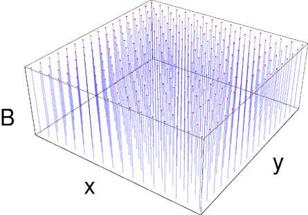
Figure 1: The sketch of the field lines of a uniform magnetic field.

$$\left[\partial_{x}^{2}-(-p_{2}+eB_{0}x)^{2}+\sigma eB_{0}\right]F_{k,p_{2},\sigma}(x)=-2|eB_{0}|kF_{k,p_{2},\sigma}(x)\;.$$ (44)

Let $\eta=\sqrt{2|eB_{0}|}(x-\frac{p_{2}}{eB_{0}})$. Then the above expression acquires the form

$$\left[\frac{\partial^{2}}{\partial\eta^{2}}+k+\frac{\sigma}{2}\text{sgn}(eB_{0})-\frac{\eta^{2}}{4}\right]F_{k,p_{2},\sigma}(\eta)=0\;,$$ (45)

that is, the equation for a quantum harmonic oscillator, with center of oscillation in $x_{0}=p_{2}/(eB_{0})$ and cyclotron frequency $w_{c}=2eB_{0}$. Thus, the normalized functions $E_{p,\sigma}$ acquire the form

$$E_{p,1} = \frac{(\pi|eB_{0}|)^{1/4}}{2\pi^{3/2}k!^{1/2}}e^{-ip_{0}t+ip_{2}y}D_{k}(\eta)\;,$$

$$E_{p,-1} = \frac{(\pi|eB_{0}|)^{1/4}}{2\pi^{3/2}(k-1)!^{1/2}}e^{-ip_{0}t+ip_{2}y}D_{k-1}(\eta)\;,$$ (46)

where

$$D_{n}(x)=2^{-n/2}e^{-x^{2}/4}H_{n}\left(x/\sqrt{2}\right)$$ (47)

is the parabolic cylinder function of order

$$n=k+\frac{\sigma}{2}\text{sgn}(eB_{0})-\frac{1}{2}\;,$$ (48)

and $H_{n}(x)$ are the Hermite’s polynomials. Expectedly, the uniform magnetic field renders the $(n-1)$-th state with spin down with the same energy of the $n$-th state with spin up. In Fig. 2, we depicted the functions $E_{p}\equiv E_{p,1}$ along the dynamical direction for various Landau levels.

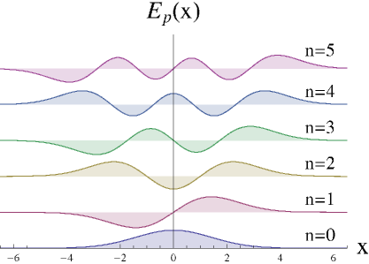
Figure 2: The $E_{p}$ functions, Eq.(46), in arbitrary units along the dynamical direction for various Landau levels. The scale of the graphic is set by $eB_{0}=1$ and $p_{2}=0$.

As we mentioned before, the Ritus eigenfunctions correspond to the asymptotic states of electrons in the presence of a magnetic field. Therefore, physical observables like probability densities are linear combinations of $|E_{p}|^{2}$. These functions have the profile shown Fig. 3. The solid curve enveloping these solutions corresponds to the potential

$$y=\bar{W}^{2}(x)-\bar{W}^{\prime}(x)\;,$$ (49)

where $\bar{W}=eW-p_{2}$ is referred to as the superpotential in the SUSY-QM literature. susyqm

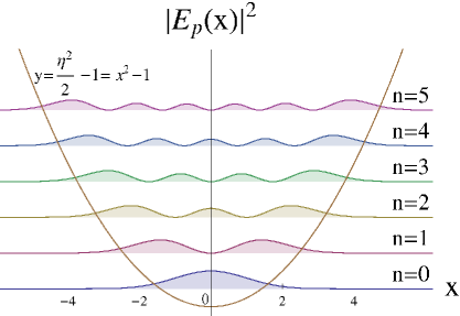
Figure 3: The $|E_{p}|^{2}$ function from Eq. (46) in arbitrary units along the dynamical direction for various Landau levels. The curve $y=x^{2}-1$ corresponds to the potential (49) for this field configuration. The scale of the graphic is set by $eB_{0}=1$ and $p_{2}=0$.

IV.2 Exponential Magnetic Field

There are many problems relating electrons in non-uniform magnetic fields of relevance in graphene. In particular, it has been established the possibility to confine quasiparticles in magnetic barriers. gaby This could be feasible creating spatially inhomogeneous, but constant in time, magnetic fields depositing ferromagnetic layers over the substrate of a graphene sample layer. Reijniers The physical properties of graphene make it a promising novel material to control the transport properties in nanodevices. It has been considered to be used in electronics and spintronics applications, like in single-electron transistors, Ponomarenko in the so called magnetic edge states, Park which may play an important role in the spin-polarized currents along magnetic domains, and in quantum dots and antidots magnetically confined. Moreover, the quantum Hall effect in graphene has been observed at room temperature, Novoselov2 evidence which confirms the great potential of graphene as the material to be used in carbon-based electronic devices.

Here we study the electron propagator in a background static magnetic field which has an exponentially decaying spatial profile along one direction, described through the function $W(x)=-B_{0}\exp\{-\alpha x\}$. The field lines of such magnetic configuration are sketched in Fig. 4. In this case, Eq. (26) simplifies to

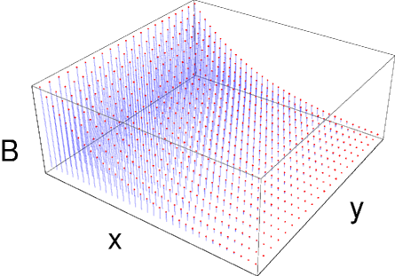
Figure 4: The sketch of the field lines of an exponentially decaying static magnetic field.

$$\left[\partial_{x}^{2}-(-p_{2}-eB_{0}\exp\{-\alpha x\})^{2}+\sigma\alpha eB_{0}\exp\{-\alpha x\}\right]F_{k,p_{2},\sigma}(x)=-kF_{k,p_{2},\sigma}(x)\;.$$ (50)

Let $\varrho=(2eB_{0}/\alpha)\exp\{-\alpha x\}$ and $s=-p_{2}/\alpha$, then, the above expression is equivalent to

$$\left[\varrho^{2}\frac{\partial^{2}}{\partial\varrho^{2}}+\varrho\frac{\partial}{\partial\varrho}-\left(s-\frac{1}{2}\varrho\right)^{2}+\frac{\sigma}{2}\varrho+\frac{k}{\alpha^{2}}\right]F_{k,p_{2},\sigma}(\varrho)=0\;.$$ (51)

This equation has the normalized solutions $E_{p,\sigma}$ given as

$$E_{p,1} = \frac{1}{2\pi}\left(\frac{2\alpha n!(s-n)}{\Gamma(2s-n+1)}\right)^{1/2}e^{-ip_{0}t+ip_{2}y}e^{-\varrho/2}\varrho^{(s-n)}L_{n}^{2(s-n)}(\varrho),$$

$$E_{p,-1} = \frac{1}{2\pi}\left(\frac{2\alpha(n-1)!(s-n)}{\Gamma(2s-n)}\right)^{1/2}e^{-ip_{0}t+ip_{2}y}e^{-\varrho/2}\varrho^{(s-n)}L_{n-1}^{2(s-n)}(\varrho),$$ (52)

where $L_{a}^{b}(x)$ are the associate Laguerre polynomials with

$$n=s-\sqrt{-\frac{k}{\alpha^{2}}+s^{2}}.$$ (53)

The quantum number $n$ is the principal quantum number, whereas $s$ a center of oscillation weighted by the damping factor $\alpha$. The solutions $E_{p}$ from Eq. (52) are sketched in Figs. 5-7 for $n=0,1$ and 2 for various values of $s$, whereas in Fig. 8 we show $|E_{p}|^{2}$ for various values of $n$ at fixed $s=8$. Notice that in this case the potential (49) also envelops the squares of the solutions.

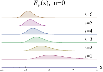
Figure 5: The $E_{p}$ functions from Eq. (52) in arbitrary units along the dynamical direction for various values of $s$ at fixed $n=0$. The scale of the graphic is set by $eB_{0}=\alpha=1$.

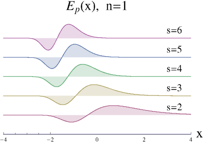
Figure 6: The $E_{p}$ functions from Eq. (52) in arbitrary units along the dynamical direction for various values of $s$ at fixed $n=1$. The scale of the graphic is set by $eB_{0}=\alpha=1$.

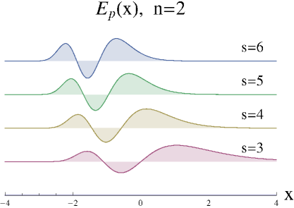
Figure 7: The $E_{p}$ functions from Eq. (52) in arbitrary units along the dynamical direction for various values of $s$ at fixed $n=2$. The scale of the graphic is set by $eB_{0}=\alpha=1$.

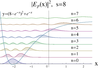
Figure 8: The $|E_{p}|^{2}$ functions from Eq. (52) in arbitrary units along the dynamical direction for various values of $n$ at fixed $s=8$. The curve $y=(8-e^{-x})^{2}+e^{-x}$ corresponds to the potential (49) for this field configuration. The scale of the graphic is set by $eB_{0}=\alpha=1$.

This concludes our presentation of the Ritus method in magnetic fields. In the next section we consider the Schwinger model for electric fields within this approach.

V Propagator in Electric Fields

The Dirac equation in the massive Schwinger model Schwinger takes the form shown in Eq. (11), but only two $\gamma^{\mu}$-matrices are involved. In this section, we work in a (1+1)-dimensional Minkowski space with metric $g^{\mu\nu}=g_{\mu\nu}=\text{diag}(1,-1)$, again in natural units. We choose the $\gamma^{\mu}$-matrices as

$$\gamma_{0}=\left(\begin{tabular}[]{c c}0&1\\ 1&0\end{tabular}\right)\;,\qquad\gamma_{1}=\left(\begin{tabular}[]{c c}0&-1\\ 1&\phantom{-}0\end{tabular}\right)\;.$$ (58)

Notice that

$$\gamma_{5}=\gamma_{0}\gamma_{1}=\left(\begin{tabular}[]{c c}1&\phantom{-}0\\ 0&-1\end{tabular}\right)\equiv\sigma_{01}\;.$$ (61)

We introduce a constant uniform electric field in the gauge

$$A_{\mu}=(-E_{0}x,0)\;,$$ (62)

and then, since the only non-vanishing components of the field strength tensor are $F_{01}=-F_{10}=E_{0}$, we have that

$$(\gamma\cdot\Pi)^{2}{\mathbb{E}}_{p} = \left[\Pi^{2}-ie\gamma_{5}E_{0}\right]\mathbb{E}_{p}\ =\ p^{2}\mathbb{E}_{p}\;.$$ (63)

We look for solutions of the form

$$\mathbb{E}_{p} = E_{p,\sigma}(t,x)\omega_{\sigma}\ =\ e^{-ip_{0}t}\ E_{p,\sigma}(x)\omega_{\sigma}\;,$$ (64)

where $\omega_{\sigma}$ is the matrix of eigenvectors of $\gamma_{5}$ with eigenvalues $\sigma=\pm 1$, respectively. Explicitly, the Ritus eigenfunctions for this problem are of the form

$$\mathbb{E}_{p}=e^{-ip_{0}t}\left(\begin{tabular}[]{c c}$E_{p,1}(x)$&0\\ 0&$E_{p,-1}(x)$\end{tabular}\right)\;,$$ (67)

where the $E_{p,\sigma}$ functions verify

$$\left[-(\partial_{t}+ieE_{0}x)^{2}+\partial_{x}^{2}-ie\sigma E_{0}\right]E_{p,\sigma}=p^{2}E_{p,\sigma}\;.$$ (68)

Let us make the replacement $p^{2}\to 2ieE_{0}p^{2}$ as in the case of a uniform magnetic field. Then making the change of variables $E_{0}\rightarrow i{\cal E}_{0}$ and $\rho=\sqrt{2e{\cal E}_{0}}\left(x+ip_{0}/(e{\cal E}_{0})\right)$, we get

$$\left[\frac{\partial^{2}}{\partial\rho^{2}}+p^{2}+\frac{\sigma}{2}-\frac{\rho^{2}}{4}\right]E_{p,\sigma}(\rho)=0\;,$$ (69)

which is again a displaced harmonic oscillator with center of oscillation in $x_{0}=ip_{0}/(e{\cal E}_{0})$ and frequency $\omega_{c}=2e{\cal E}_{0}$. Thus the solutions are again parabolic cylinder functions

$$E_{p,1}(\rho) = \frac{(2e{\cal E}_{0})^{1/4}}{(2\pi)^{3/2}(n+1)!^{1/2}}D_{n+1}(\rho)\;,$$

$$E_{p,-1}(\rho) = \frac{(2e{\cal E}_{0})^{1/4}}{(2\pi)^{3/2}n!^{1/2}}D_{n}(\rho)\;,$$ (70)

of order

$$n=p^{2}+\frac{\sigma}{2}-\frac{1}{2}.$$ (71)

Contrary to the case of the uniform magnetic field, the arguments of the parabolic cylinder functions as well as the order, are complex numbers. Nevertheless, they serve as well to diagonalize the propagator as

$$S(x)=\int dp\ \mathbb{E}_{p}(x)\frac{1}{\gamma\cdot\overline{p}-m}\overline{\mathbb{E}}_{p}(x)\;,$$ (72)

which is found through the relation (29) with $\overline{p}_{\mu}=(p,0)$, where $p$ is defined in Eq. (71).

This illustrates the usefulness of the Ritus method. Below we present a discussion and the conclusions.

VI Discussion and conclusions

In this paper we have reviewed the massive electron propagator in lower than (3+1) space-time dimensions. We have obtained the free electron propagator through the Green’s function method in arbitrary dimensions and has, as we know, a diagonal form in momentum space, namely $S_{F}(p)=1/(\gamma\cdot p-m)$. This is obviously the case because the free Dirac operator commutes with the momentum operator and thus one can take simply a Fourier transform, that is to say, we can use the eigenfunctions of the momentum operator to diagonalize the Green’s function.

We have then considered the electron propagator in (2+1)-dimensions in an external magnetic field pointing perpendicularly to the plane of motion of the electron and whose spatial shape we considered described by some arbitrary function $W(x)$. This, to the best of our knowledge, has been presented for the first time in literature. We selected to work within the Ritus method Ritus framework, and construct explicitly the eigenfunctions ${\mathbb{E}}_{p}$ of the $\left(\gamma\cdot\Pi\right)^{2}$ operator in the general case. The basic idea behind this method is the following: since the Dirac operator $\left(\gamma\cdot\Pi\right)$ does not commute with the momentum operator, we cannot simply take the Fourier transform of the Green’s function and have a diagonal propagator in momentum space. However since $\left(\gamma\cdot\Pi\right)$ commutes with $i\partial_{t}$, $-i\partial_{y}$ and, more importantly, with $\left(\gamma\cdot\Pi\right)^{2}$, we can use their common eigenfunctions, ${\mathbb{E}}_{p}$, to diagonalize the propagator, which turns out to have the form of a free propagator with momentum depending upon the dynamical quantum numbers. We have specialized our findings to the case of a uniform magnetic field where the ${\mathbb{E}}_{p}$ functions are described in terms of parabolic cylinder functions. As a second example, we considered an exponentially damped static magnetic field. Here the Ritus eigenfunctions are written in terms of associate Legendre functions. On both these cases, the massless versions of the propagators are of direct relevance in graphene.

We also considered the propagator in (1+1)-dimensions in a uniform electric field. Our findings in this case are similar to the magnetic field case in the plane, except that the eigenfunctions have complex arguments and order. The important lesson here is that the method works in arbitrary dimensions and different field configurations. In each case, the propagator continues to have a diagonal form, although the ${\mathbb{E}}_{p}$ functions change from one configuration to the other.

In conclusion, the Ritus method offers an alternative to study the electron propagator in the presence of external fields. Contrary to the “proper time” method Fock ; Schwinger , the propagator here acquires its free form, and the effects of the field are reflected in the eigenfunctions of the operator $\left(\gamma\cdot\Pi\right)^{2}$, namely ${\mathbb{E}}_{p}$. The method works as well in the case of scalar scalar and vector charged particles. vector The idea behind it is familiar in quantum mechanics, where the diagonalization of a given operator is carried out with the aid of eigenfunctions of a second commuting operator. That makes Ritus method suitable to study the propagator for more complex configurations of external fields.

Project

For the interested reader, we propose the following project: Work out the derivation of the propagator in (2+1)-dimensions in a magnetic field making use of the second irreducible representation of the Dirac matrices, Eq.(9), and show that in this case, the ${\mathbb{E}}_{p}$ functions have the form

$${\mathbb{E}}_{p}=\left(\begin{array}[]{cc}E_{p,-1}(z)&0\\ 0&E_{p,1}(z)\end{array}\right)\;.$$ (73)

- (1) L.D. Landau, Paramagnetism of metals, Z. Phys. 64, 629-637 (1930).
- (2) F.A. Barone, H. Boschi-Filho and C. Farina, Three methods for calculating the Feynman propagator, Am. J. Phys. 71, 483-491 (2003); A. Aragão, H. Boschi-Filho, C. Farina and F. A. Barone, Non-relativistic propagators via Schwinger’s method, Braz. J. Phys. 37, 1260-1268 (2007).
- (3) V.A. Fock, Die Eigenzeit in der klassischen und in der Quantenmechanik, Phys. Z. Sowjetunion 12, 404-425 (1937).
- (4) J. Schwinger, On gauge invariance and vacuum polarization, Phys. Rev. 82, 664-679 (1951).
- (5) C. Itzykson and J. Zuber, Quantum field theory, (McGraw-Hill Inc. 1980) pp. 100-104.
- (6) L.F. Urrutia and E. Hernández, Calculation of the propagator for a time-dependent damped, forced harmonic oscillator using the Schwinger action principle, Int. J. Theor. Phys. 23, 1105-1127 (1984); L.F. Urrutia and C. Manterola, Propagator for the anisotropic three-dimensional charged harmonic oscillator in a constant magnetic field using the Schwinger action principle, Int. J. Theor. Phys. 25, 75-88 (1986); N. J. M. Horing, H. L. Cui and G. Fiorenza, Nonrelativistic Schrodinger Greens function for crossed time dependent electric and magnetic fields, Phys. Rev. A34, 612-615 (1986); C. Farina and Antonio Segui-Santonja, Schwinger’s method for a harmonic oscillator with a time-dependent frequency, Phys. Lett. A184, 23-28 (1993).
- (7) J. Suzuki, Quantum electrodynamics in a uniform magnetic field, arXiv:hep-th/0512329v1; K. Battacharya, Solution of the Dirac equation in presence of an uniform magnetic field, arXiv:0705.4275v2 [hep-th].
- (8) K.-M. Poon and G. Muñoz, Path integrals and propagators for quadratic lagrangians in three dimensions, Am. J. of Phys. 67, 547-551 (1999).
- (9) V. I. Ritus, Radiative corrections in quantum electrodynamics with intense field and their analytical properties, Ann. Phys. 69, 555-582 (1972); V. I. Ritus, On diagonality of the electron mass operator in the constant field, Pizma Zh. E. T. F. 20, 135-138 (1974) [in Russian]; V. I. Ritus, The eigenfunction method and the mass operator in quantum electrodynamics of the constant field, Zh. E. T. F. 75, 1560-1583 (1978) [in Russian].
- (10) G. W. Semenoff, Condensed-matter simulation of a three-dimensional anomaly, Phys. Rev. Lett. 53, 2499-2452 (1984); D. P. Di Vicenzo and E. J. Mele, Self-consistent effective-mass theory for intralayer screening in graphite intercalation compounds, Phys. Rev B29, 1685-1694 (1984).
- (11) K.S. Novoselov, A.K. Geim, S.V. Morozov, D. Jiang, M.I. Katsnelson, I.V. Grigorieva, S.V. Dubonos and A.A. Firsov, Two-dimensional gas of massless Dirac fermions in Graphene, Nature (London) 438, 197-200 (2005); Y, Zhang, Y.-W. Tan, H. L. Stormer and P. Kim, Experimental observation of quantum Hall effect and Berry’s phase in Graphene, Nature (London) 438, 201-204 (2005).
- (12) A.K. Geim and K.S. Novoselov, The rise of Graphene, Nature Materials 6, 183-191 (2007).
- (13) C.G. Beneventano, P. Giacconi, E. M. Santangelo, and Roberto Soldati, Planar QED at finite temperature and density: Hall conductivity, Berry’s phases and minimal conductivity of Graphene, J. Phys. A 42, 275401, 1-25 (2009).
- (14) V. R. Khalilov, QED2+1 radiation effects in a strong magnetic field, Theor. and Math. Phys. 121, 1606-1616 (1999).
- (15) We use a prescription for which for any vector in -dimensions.
- (16) N. M. Peres, F. Guinea and A. H. Castro Neto, Electronic properties of disordered two-dimensional carbon, Phys. Rev. B73, 125411, 1-23 (2006).
- (17) V.L. Ginzburg (Editor), Quantum electrodynamics with unstable vacuum, 1st. Edition (Nova Science Publishers, Inc. 1995) pp. 155-161.
- (18) E. Elizalde, E. Ferrer and V. de la Incera, Neutrino self-energy and index of refraction in strong magnetic field: A new approach, Ann. Phys. 295, 33-49 (2002).
- (19) F. Cooper, A. Khare and U. Shukhatme, Supersymmetry and quantum mechanics, Phys. Rep. 251, 267-385 (1995). F. Cooper, A. Khare and U. Shukhatme, Supersymmetry in quantum mechanics, 1st. Edition (World Scientific Publishing Co. Pte. Ltd. 2001) pp. 61-80.
- (20) A. De Martino, L. Dell’Anna and R. Egger, Magnetic confinement of massless Dirac fermions in Graphene, Phys. Rev. Lett. 98, 066802, 1-4 (2007); M. Ramezani Masir, A. Matulis and F. M. Peeters, Quasibound states of Schrödinger and Dirac electrons in a magnetic quantum dot, Phys. Rev. B 79, 155451, 1-8 (2009).
- (21) J. Reijniers, F. M. Peeters and A. Matulis, Electron scattering on circular symmetric magnetic profiles in a two-dimensional electron gas, Phys. Rev. B 64, 245314, 1-8 (2001).
- (22) L. A. Ponomarenko, F. Schedin, M. I. Katsnelson, R. Yang, E. W. Hill, K. S. Novoselov and A. K. Geim, Chaotic Dirac Billiard in Graphene Quantum Dots, Science 320, 356-358 (2008); X. Wu, M. Sprinkle, X. Li, F. Ming, C. Berger and W. A. de Heer, Epitaxial-Graphene/Graphene-Oxide Junction: An Essential Step towards Epitaxial Graphene Electronics, Phys. Rev. Lett. 101, 026801, 1-4 (2008).
- (23) S. Park and H.-S. Sim, Magnetic edge states in graphene in nonuniform magnetic fields, Phys. Rev. B 77, 075433, 1-8, (2008).
- (24) K. S. Novoselov, Z. Jiang, Y. Zhang, S. V. Morozov, H. L. Stormer, U. Zeitler, J. C. Maan, G. S. Boebinger, P. Kim and A. K. Geim, Room-Temperature Quantum Hall Effect in Graphene, Science 315, 1379-1379, (2007).