Constructing classical field for a Bose-Einstein condensate in arbitrary trapping potential; quadrupole oscillations at nonzero temperatures

Abstract

We optimize the classical field approximation of the version described in J. Phys. B 40, R1 (2007) for the oscillations of a Bose gas trapped in a harmonic potential at nonzero temperatures, as experimentally investigated by Jin et al. [Phys. Rev. Lett. 78, 764 (1997)]. Similarly to experiment, the system response to external perturbations strongly depends on the initial temperature and on the symmetry of perturbation. While for lower temperatures the thermal cloud follows the condensed part, for higher temperatures the thermal atoms oscillate rather with their natural frequency, whereas the condensate exhibits a frequency shift toward the thermal cloud frequency ($m=0$ mode), or in the opposite direction ($m=2$ mode). In the latter case, for temperatures approaching critical, we find that the condensate begins to oscillate with the frequency of the thermal atoms, as in the $m=0$ mode. A broad range of frequencies of the perturbing potential is considered.

I Introduction

Experiments with atomic Bose-Einstein condensates driven by an external perturbation have allowed verification of the mean-field description of the condensed phase in a dynamical regime where the system responds by collective motion. Typically, a periodic perturbation (with a particular symmetry) of a trapping potential was used to excite the Bose gas Cornell-zero ; Ketterle-zero ; Cornell-osc ; Ketterle-osc , although other kinds of trap distortion leading, for instance, to scissors mode excitations Foot or the transverse monopole mode excitation in an elongated condensateDalibard were also tried. The investigation of the low energy collective modes of the condensate in the zero-temperature limit Cornell-zero ; Ketterle-zero has revealed that the mean-field description of that system (i.e., based on the Gross-Pitaevskii equation) works well theory-zero . However, when the study of low-lying excitations was extended to include the measurement of frequencies and damping rates as a function of temperature Cornell-osc ; Ketterle-osc , it became clear that a new theory of an interacting Bose gas at nonzero temperatures is required.

The JILA experiment of Ref. Cornell-osc showed two effects. First, it was found that two collective modes with different symmetries (quadrupole modes with angular momenta equal to $m=0$ and $m=2$) behave in qualitatively different ways. When the temperature increases, they exhibit a frequency shift in opposite directions. Moreover, for the $m=0$ mode a rather sudden upward shift is observed, suggesting the existence of a characteristic temperature which is approximately $0.65$ of the critical temperature for the corresponding ideal gas. Secondly, the damping of the collective oscillations turned out to be dramatically dependent on temperature, showing that the condensate modes are damped even faster than the noncondensed fraction while approaching the critical temperature. All these puzzling findings triggered a lot of theoretical work and after a few years resulted in the development of Zaremba-Nikuni-Griffin formalism ZNG ; Zaremba-osc and the second-order quantum field theory Burnett-osc ; Morgan for a Bose gas. Recently, another attempt to describe finite-temperature properties of low-lying collective modes was undertaken in Ref. Blakie-osc within the approximation called the projected Gross-Pitaevskii equation.

The Zaremba-Nikuni-Griffin formalism Zaremba-osc applied to the results of the JILA experiment gives relatively good agreement. Also the calculations based on the second-order quantum field theory Burnett-osc show a good agreement with experimental data. However, already these two approaches differ when considering their fundamentals. For example, the first one neglects the phonon character of the low-lying energy modes, the anomalous average, as well as the Beliaev processes. Regarding the JILA experiment, for the $m=0$ mode, the Zaremba-Nikuni-Griffin method predicts an additional branch of condensate frequencies, so far not observed experimentally. No such branch is found within the second-order theory of Ref. Burnett-osc . Furthermore, this approach predicts a single frequency of condensate response for a particular temperature, regardless of driving frequency, and hence the notion of a natural condensate frequency is meaningful. This strongly differs from what is reported in Jackson and Zaremba Zaremba-osc , where the condensate response depends on the driving frequency of the whole system (condensed and noncondensed parts). A comprehensive discussion of both approaches in the context of JILA experiment can be found in a recent review article Proukakis . Another formalism, based on the projected Gross-Pitaevskii equation, used to model the JILA experiment Cornell-osc produces good agreement with experimental data up to $0.65T_{c}$, and for the $m=2$ mode at higher temperatures. However, it fails to predict the sudden upward frequency shift for the $m=0$ mode at this temperature Blakie-osc . This failure is perhaps related to the way the cutoff parameter (which splits the space of modes into the highly occupied ones that are described in terms of the classical field, and the others that are sparsely occupied and require, in principle, a quantum treatment) is chosen. The details of the splitting procedure within the projected Gross-Pitaevskii equation approach are discussed in Ref. Advances .

In this paper we apply the classical field approximation in the version described in Ref. przeglad to the case of a trapped interacting Bose gas at nonzero temperatures driven by an external perturbation as in the experiment of Ref. Cornell-osc . The main purpose of this work is to check whether the classical field approximation is able to reproduce, at least qualitatively, the findings of JILA experiment. This is an especially important task because of the recently reported failure Blakie-osc to explain the behavior of the $m=0$ mode within the projected Gross-Pitaevskii equation method, which is conceptually very close to our classical field approximation. On the other hand, although the other existing theories Zaremba-osc and Burnett-osc both lead to relatively good agreement with the experiment Cornell-osc , they somehow contradict each other conceptually as discussed in the previous paragraph. It would be nice to have an alternative view of the processes going on in the perturbed Bose gas. Finally, the approaches Zaremba-osc and Burnett-osc have some difficulties in describing the dynamics of the thermal cloud, especially in the $m=2$ mode. In fact, no predictions for thermal component frequencies in the $m=2$ mode are given in Zaremba-osc or Burnett-osc . Simultaneously, within the projected Gross-Pitaevskii equation method, at higher temperatures, the thermal cloud (in fact, for both the $m=0$ and $m=2$ modes) oscillates at frequencies much lower than in experiment.

The classical field approximation has already been applied in static and dynamical regimes for a uniform and harmonically trapped systems (for a review, see przeglad ). This approach was used to investigate the thermodynamics of an interacting gas rapid ; JPB as well as dynamical processes like the photoassociation of molecules photo , the dissipative dynamics of a vortex vortex1 , the superfluidity in ring-shaped traps super , or the thermalization in spinor condensates spinor . The classical field approximation was also tested at a quantitative level when e.g. the Bogoliubov-Popov quasiparticle energy spectrum in a uniform Bose gas was obtained JPB or when the process of splitting of doubly quantized vortices in dilute Bose-Einstein condensates vortex2 was studied.

The paper is organized as follows: In Sec. II we describe the classical field approximation for a trapped Bose gas with particular attention on how the equilibrium state is obtained and on the quality of the solution in comparison with the equilibrium states calculated within the self-consistent Hartree-Fock method. Sec. III discusses the results (response frequencies and damping rates) for the quadrupole $m=0$ collective mode for parameters as in JILA experiment Cornell-osc while in Sec. IV we do the same for $m=2$ excitation. Finally, we conclude in Sec. V.

II Classical field approximation for a trapped Bose gas

II.1 Formalism

A good starting point to introduce the classical field approximation is the usual Heisenberg equation of motion for the bosonic field operator $\hat{\Psi}({\bf r},t)$ which annihilates an atom at point ${\bf r}$ and time $t$. The field operator $\hat{\Psi}({\bf r},t)$ fulfills standard commutation relations:

$$\left[{\hat{\Psi}({\rm{\bf r}},t),\hat{\Psi}^{+}({\rm{\bf r}^{\prime}},t)}\right]=\delta({\rm{\bf r}}-{\rm{\bf r}^{\prime}})$$ (1)

with other equal time commutation relations for $[\hat{\Psi},\hat{\Psi}]$ and $[\hat{\Psi}^{+},\hat{\Psi}^{+}]$ being zeros. The equation of motion reads:

$$i\hbar\frac{\partial}{\partial t}\hat{\Psi}({\rm{\bf r}},t)=\left[-\frac{\hbar^{2}}{2m}\nabla^{2}+V_{tr}({\rm{\bf r}},t)\right]\hat{\Psi}({\rm{\bf r}},t)$$

$$+g\,\hat{\Psi}^{+}({\rm{\bf r}},t)\hat{\Psi}({\rm{\bf r}},t)\hat{\Psi}({\rm{\bf r}},t)\,.$$ (2)

Here, we assume the time-dependent trapping potential $V_{tr}$ and the usual contact interaction for colliding atoms. The coupling constant $g=4\pi\hbar^{2}a/m$ is expressed in terms of the s-wave scattering length $a$.

Next, we expand the field operator $\hat{\Psi}({\bf r},t)$ in the basis of one-particle wave functions $\psi_{k}({\bf r})$, where $k$ is a set of one-particle quantum numbers:

$$\hat{\Psi}({\rm{\bf r}},t)=\sum_{k}\psi_{k}({\bf r})\hat{a}_{k}(t)$$ (3)

Now, we assume that some of the modes used in the expansion (3) are macroscopically occupied and extend the original Bogoliubov idea Bogoliubov by replacing all operators $\hat{a}_{k}(t)$ corresponding to these modes by c-numbers. When only macroscopically occupied modes are considered, the field operator $\hat{\Psi}({\bf r},t)$ is turned into the complex wave function $\Psi({\bf r},t)$ and the expansion (3) takes the form:

$$\Psi({\rm{\bf r}},t)=\sum_{k=0}^{k_{max}}\psi_{k}({\bf r})a_{k}(t)\,.$$ (4)

The upper index in the summation tells us that, indeed, the wave function $\Psi({\bf r},t)$ is expanded only over a finite number of states, i.e. those which are macroscopically occupied. We call the wave function $\Psi({\bf r},t)$ the classical field. This is analogous to the way that intense electromagnetic waves can be treated. In spite of consisting of photons, an intense light beam is well characterized by the classical electric and magnetic fields. Since the experiments with dilute atomic gases are performed with millions of atoms it seems to be a plausible approximation to use the classical field to describe atoms in analogy with electric and magnetic fields for photons.

Obviously, the classical field obeys the following equation:

$$i\hbar\frac{\partial}{\partial t}{\Psi}({\rm{\bf r}},t)=\left[-\frac{\hbar^{2}}{2m}\nabla^{2}+V_{tr}({\rm{\bf r}},t)\right]{\Psi}({\rm{\bf r}},t)$$

$$+g\,{\Psi}^{*}({\rm{\bf r}},t){\Psi}({\rm{\bf r}},t){\Psi}({\rm{\bf r}},t)\,.$$ (5)

We usually implement the cutoff parameter $k_{max}$ by solving the Eq. (5) on a rectangular grid using the Fast Fourier Transform technique. The spatial grid step determines the maximal momentum per particle (and hence the energy) in the system whereas the use of the Fourier transform implies a projection in momentum space.

The equation (5) looks like the usual Gross-Pitaevskii equation describing the Bose-Einstein condensate at zero temperature. However, here the interpretation of the complex wave function $\Psi({\bf r},t)$ is different. It describes all the atoms in the system, both those in a condensate and in a thermal cloud. Therefore, the question appears how to split the classical field $\Psi({\bf r},t)$ into the condensed and noncondensed fractions. For that we use the definition of a Bose-Einstein condensation proposed originally by Penrose and Onsager POdef . According to this definition the condensate is assigned to the eigenvector corresponding to the dominant eigenvalue of a one-particle density matrix. So, we built the one-particle density matrix in the following way:

$$\rho^{(1)}({\bf r},{\bf r}^{\,\prime};t)=\frac{1}{N}\,\Psi({\bf r},t)\,\Psi^{*}({\bf r}^{\,\prime},t)\,,$$ (6)

where $N$ is the total number of particles. However, and here comes the surprise – since (6) is just the spectral decomposition of a one-particle density matrix, this would imply that the classical field $\Psi({\bf r},t)$ is the condensate wave function and that all atoms are in the condensate. To split the classical field into the condensed and thermal fractions one first realizes that the high energy solutions of Eq. (5) oscillate rapidly in time and space. On the other hand, the detection process is always performed with limited spatial and temporal resolution. Therefore, it becomes clear that the measurement process with its limited resolution involves a kind of averaging (coarse-graining) of Eq. (6). Again, an analogy with electromagnetic waves is in place. A partially coherent light beam exhibits complicated spatial and temporal behavior on short scales, in fact too complicated to be typically measured. What is important are then the correlation functions at long enough spatial and temporal separation, averaged over the smaller time intervals and space segments. Similarly here, the averaging over time and/or space of the one-particle density matrix (6) results in a partial loss of the information contained in the classical field rapid . In other words, the mixed state emerges out of the pure one.

In a typical experiment, what is measured is the column density along some direction. Hence, we also implement the coarse-graining procedure in our numerics in this manner as:

$$\bar{\rho}(x,y,x^{\prime},y^{\prime};t)=\frac{1}{N}\int dz\,\Psi(x,y,z,t)\,\Psi^{*}(x^{\prime},y^{\prime},z,t)\,.$$ (7)

Solving the eigenvalue problem for a coarse-grained density matrix (7) results in a decomposition:

$$\bar{\rho}=\sum_{k}n_{k}\,\varphi_{k}(x,y,t)\,\varphi^{*}_{k}(x^{\,\prime},y^{\,\prime},t)\,,$$ (8)

where $n_{k}=N_{k}/N$ are the relative occupations of macroscopically occupied modes $\varphi_{k}$. Defining the dominant eigenvalue as $n_{0}$, the condensate wave function (normalized to $N_{0}/N$) can be written as:

$$\psi_{0}(x,y,t)=\sqrt{\frac{N_{0}}{N}}\,\varphi_{0}(x,y,t)\,.$$ (9)

All the other modes contribute to the thermal density which is, therefore, given by:

$$\rho_{T}(x,y,t)=\bar{\rho}(x,y,x,y;t)-|\psi_{0}(x,y,t)|^{2}\,.$$ (10)

The appropriateness of the averaging (7) for obtaining the large eigenvalues of a coarse-grained density matrix was verified by us in various ways. For example, we checked that for the classical field at equilibrium this procedure gives the same results as averaging over a long enough time. Prescription (7) also works at zero temperature (when all atoms are expected to be in a condensate), having been successfully tested in this respect in the demanding case of a lattice of bent vortices (see Ref. mcv for further details).

According to the description given above the splitting of the system into condensed and noncondensed components is a result of Bose statistics, interaction, and the measurement process. Unlike the alternative approaches ZNG ; Burnett-osc we do not impose a two-component character of the system from the beginning. Also, our version of the classical field method is well suited to describe single realizations of the experiment since it corresponds to a microcanonical ensemble, as opposed to the competing approach CastinCFA , which deals with canonical ensembles.

II.2 Obtaining equilibrium states

An initial classical field is generated from the ground state solution of Eq. (5) by adding appropriate random disturbance. An inspection of that equation indicates that only the product of the coupling constant $g$ and the total number of atoms $N$ enters it. Therefore, we normalize the initial classical field $\Psi({\bf r},t=0)$ to unity. The norm of $\Psi({\bf r},t)$ is then one of the constants of motion of Eq. (5). Another constant of motion is the total energy. Such an initial state is then propagated according to Eq. (5) until the constituent energies (kinetic, trap, and interaction) cease to change systematically in time and exhibit only fluctuations. In this way the classical field at thermal equilibrium, corresponding to the particular values of $gN$ and $E_{tot}/N$, is obtained. An example is given in Fig. 1, where we plot cuts of the total density, the condensate, and the thermal densities according to the prescription detailed in the previous section. Here, the equilibrium classical field describes a degenerate ⁸⁷Rb Bose gas in a magnetic trap with frequencies $\omega_{\bot}\equiv\omega_{x,y}=2\pi\times 129\,$Hz and $\omega_{z}=2\pi\times 365\,$Hz as in the experiment of Ref. Cornell-osc . Other parameters are: $gN=2911.9$ and $E_{tot}/N=21.2$ in units of $\hbar\omega_{z}(\hbar/m\omega_{z})^{3/2}$ and $\hbar\omega_{z}$, respectively. They result in a condensate fraction $n_{0}=0.3$. A bimodal distribution (thick solid line) is clearly visible.

Figure 1: Cuts of the total (thick solid line), condensate (dashed line), and thermal (thin solid line) densities as obtained by integrating a one-particle density matrix along the direction of imaging and then applying the splitting procedure described in Sec. II.1. Note the bimodal character of the density distribution (here, the condensate fraction equals $0.3$). The oscillatory unit of length is defined via the axial trap frequency: $\sqrt{\frac{\hbar}{m\omega_{z}}}$ and equals $0.565\,\mu m$.

Now we have to solve the problem how to find the number of particles assigned to the classical field at equilibrium and how to determine the temperature of the system. This can be done in two ways. The first is given here, the second in Sec. II.3. To begin with, having the classical field at equilibrium one can project the field $\Psi({\bf r},t)$ on the harmonic oscillator states obtaining in this way the relative populations of these states. Fig. 2 shows relative populations for $gN=1811.9$ and $E_{tot}/N=10.0$ as a function of the harmonic oscillator states’ energy (precisely, the time average over $274\,$ms is plotted). The maximal one-particle mode energy is determined by the momentum cutoff $p_{max}$ as $p_{max}^{2}/m$.

Figure 2: Relative populations of various harmonic oscillator states. The energy cutoff equals $p_{max}^{2}/m$, where $p_{max}$ is the momentum cutoff.

An important observation is made when one looks at the energy accumulated in harmonic oscillator states, see Fig. 3. For higher energy states the product $n_{i}\,\varepsilon_{i}$ (where $n_{i}$ and $\varepsilon_{i}$ are the relative population and the harmonic oscillator state energy, respectively) becomes constant. On the other hand, for highly occupied modes (i.e., modes satisfying $\epsilon_{i}-\mu\lesssim k_{B}T$, where $\mu$ is the chemical potential) the quantum Bose-Einstein distribution reduces to the classical equipartition distribution. For the classical field studied here the equipartition extends all the way to the cutoff energy:

$$N_{i}\,(\epsilon_{i}-\mu)=k_{B}T\,,$$ (11)

which can be written equivalently as

$$n_{i}\,(\epsilon_{i}-\mu)=k_{B}T/N\,.$$ (12)

Therefore, since energy equipartition is established, the higher energy harmonic oscillator states become the quasiparticle modes. In Fig. 3 we determine the ratio $k_{B}T/N$ to be $4.62\times 10^{-4}$. Having the ratio $k_{B}T/N$ we now find from Eq. (12) the relative populations of high energy quasiparticle modes. In particular, we get the relative population of the least occupied modes which belong to the classical field. In the example here, they are $2.99\times 10^{-5}$ (based on formula (12) with $k_{B}T/N$ obtained above). In Ref. EW , arguments are given that the best match between this method and the ideal Bose gas occurs when the occupation of the least occupied mode is $N_{cut}=0.46$. These are based on the comparison between the probability distribution of the ideal Bose gas and its classical field counterpart. Assuming, then that the average number of atoms in this least-occupied mode is $0.46$ we can retrieve the total number of atoms in the system and its temperature separately. For the example here, these are $N=15342$ and $T=124.1\,$nK.

Figure 3: Relative populations multiplied by the state energies for various harmonic oscillator states. The figure clearly shows that for higher energy states the equipartition of an energy is established. Therefore, the higher energy states become quasiparticle modes. The fraction $k_{B}T/N$ equals approximately $4.62\times 10^{-4}$.

Since no data on the population of the cutoff mode are available for a weakly interacting Bose gas considered here we compare in Table 1 the temperature of the system and the total number of atoms for various values of $N_{cut}$.

$N_{cut}$	$T$[nK]	$N$
0.44	119.5	14778
0.46	124.1	15342
0.48	130.4	16121
0.50	135.8	16793
0.52	141.2	17465

Table 1: Temperature and the total number of atoms obtained by projecting the classical field on the harmonic oscillator states of the example described in Sec. II.2 for different values of cutoff parameter.

II.3 Comparison with the self-consistent Hartree-Fock model

Another approach to obtain the number of atoms and the temperature of the system described by the classical field at equilibrium is based on the self-consistent Hartree-Fock method Pethick . Since this method works well for a Bose gas at equilibrium as verified experimentally in Aspect , a comparison between this model and the classical field approximation should be instructive. The Hartree-Fock description is defined by the following set of equations Pethick :

$$n_{c}({\bf r})=\frac{1}{g}\left[\mu-V_{tr}({\bf r})-2\,g\,n_{th}({\bf r})\right]$$ (13)

$$f({\bf r},{\bf p})=\left(e^{[{\bf p}^{2}/2m+V_{eff}({\bf r})-\mu]/k_{B}T}-1\right)^{-1}$$ (14)

$$n_{th}({\bf r})=\frac{1}{\lambda_{T}^{3}}\;\;g_{3/2}\left(e^{\left[\mu-V_{eff}({\bf r})\right]/k_{B}T}\right)$$ (15)

$$V_{eff}({\bf r})=V_{tr}({\bf r})+2\,g\,n_{c}({\bf r})+2\,g\,n_{th}({\bf r})$$ (16)

$$\mu=g\,n_{c}(0)+2\,g\,n_{th}(0)\,,$$ (17)

where

$$\lambda_{T}=\left(\frac{2\pi\hbar^{2}}{mk_{B}T}\right)^{1/2}$$ (18)

is the thermal de Broglie wavelength and the $g_{3/2}(z)$ function is given by the expansion:

$$g_{3/2}(z)=\sum_{n=1}^{\infty}\frac{z^{n}}{n^{3/2}}\,.$$ (19)

The basic variables in this approach are the condensate density, $n_{c}({\bf r})$, and the distribution function in phase space for thermal atoms, $f({\bf r},{\bf p})$. They are calculated according to the Eqs. (13) and (14). The thermal density, $n_{th}({\bf r})$, is just an integral of the distribution function $f({\bf r},{\bf p})$ over momenta and can be found analytically (Eq. (15)). Since both the effective potential, $V_{eff}({\bf r})$, and the chemical potential, $\mu$, appearing on the right-hand sides of Eqs. (13), (14), and (15), depend on the condensate and thermal densities the set of Eqs. (13) and (14) is well suited to be solved iteratively. For that, however, we have to first choose the temperature of the system and then keep fixed the total number of atoms (which is $N=\int d{\bf r}\,(n_{c}({\bf r})+n_{th}({\bf r}))$) during the iterations. Having the densities of condensed and noncondensed fractions one can easily calculate two important parameters: the condensate fraction and the total energy per particle. Now the strategy is as follows: find the input parameters $(N,T)$ in such a way that the condensate fraction and the total energy per atom calculated within the Hartree-Fock method match the values calculated from the classical field at equilibrium. This procedure allows one to determine the number of atoms and the temperature assigned to the classical field separately.

These parameters for the example discussed in the context of Figs. 2 and 3 are found to be $N=17306$ and $T=128.7\,$nK. These values are very close to what was obtained in the previous section with the cutoff occupation $N_{cut}=0.46$, and differ by $3.7\%$ in the temperature and $12.8\%$ in the total number of atoms. The agreement is good even though the average occupation of the highest energy modes (the last modes considered in the classical field approximation as being macroscopically occupied) was taken the same as for an ideal gas. Unfortunately, there is no data available for the average occupation of the cutoff region modes for the weakly interacting gas considered here. Changing slightly this cutoff occupation number, the agreement between both approaches to the system parameters can be made even better (for example, for $N_{cut}=0.48$ the difference is $1.3\%$ and $7.4\%$ in the temperature and the total number of atoms, respectively). In Fig. 4 the total Hartree-Fock and classical field densities are plotted together for parameters as in Figs. 2 and 3 showing a good agreement. The classical field density, however, exhibits all the fluctuations which are not present in the Hartree-Fock model.

Figure 4: Total density cuts for the self-consistent Hartree-Fock (thick line) and classical field (thin line) methods for a system with the total number of atoms $N=17306$ and the temperature $T=128.7\,$nK.

In Table 2 we again compare the parameters of the system (total number of atoms and temperature) for the methods described in this and in the previous sections. However, this time the comparison is for several different equilibrium states. All the states being compared are used later in the simulations related to JILA experiment Cornell-osc (see Secs. III and IV).

	$CFA$	$HF$
$T$[nK]	79.8	91.8
$N$	6751	11300
$T$[nK]	124.1	128.7
$N$	15342	17306
$T$[nK]	142.1	153.9
$N$	16347	18699
$T$[nK]	154.4	168.8
$N$	19313	21509
$T$[nK]	177.8	190.4
$N$	26984	27875
$T$[nK]	195.3	204.8
$N$	27770	31222
$T$[nK]	264.1	240.9
$N$	61876	43572

Table 2: Comparison (for several final equilibrium states as per Table 3) between the results (the temperature and the total number of atoms) obtained by projecting the classical field on the harmonic oscillator states as described in Sec. II.2 ($CFA$ column) and by utilizing the self-consistent Hartree-Fock method according to Sec. II.3 ($HF$ column). For $CFA$ data $N_{cut}=0.46$.

II.4 Obtaining equilibrium states on demand

In Secs. II.2 and II.3 we detailed the methods for retrieving the total number of atoms and the temperature assigned to the classical field at equilibrium. Since the product $gN$ is an initial parameter it means that the coupling constant $g$ (and consequently the scattering length $a$) is known only after the classical field is thermalized. Unfortunately, it usually differs from the value that was used to calculate an initial value of $gN$. Therefore, an approach for obtaining the classical field at equilibrium corresponding to given values of the total number of atoms and the temperature is required.

The method we have developed is rather simple although demanding from a numerical point of view. Let’s assume that we need the classical field which at equilibrium describes the system with given parameters $N$ and $T$. We start from a solution obtained from the self-consistent Hartree-Fock method corresponding to the chosen parameters. Then we build an initial classical field as follows:

$$\Psi({\rm{\bf r}},t=0)=\sqrt{n_{c}({\bf r})}+\sqrt{n_{th}({\bf r})}\,e^{i\varphi({\bf r})}$$ (20)

and randomize the phase $\varphi({\bf r})$ and the density $n_{th}({\bf r})$ in such a way that the total energy per atom in the classical field equals the corresponding energy in the Hartree-Fock model. The presence of the phase factor in the second term in (20) is necessary. Without this, the classical field suffers from a lack of kinetic energy in comparison with the Hartree-Fock method, where it is calculated from the distribution function $f({\bf r},{\bf p})$:

$$E_{kin}=\frac{1}{h^{3}}\int d{\bf r}\,d{\bf p}\,\frac{{\bf p}^{2}}{2m}f({\bf r},{\bf p})$$

$$=\frac{3k_{B}T}{2\lambda_{T}^{3}}\int d{\bf r}\,g_{5/2}\left(e^{\left[\mu-V_{eff}({\bf r})\right]/kT}\right)\,.$$ (21)

Now we evolve the classical field according to Eq. (5) and let the field thermalize. During the thermalisation, the total energy per atom is a constant of motion, but the condensate fraction usually changes. However, there will be a particular value of the spatial step of the grid for which the condensate fraction does not change in time. Then, since the total energy per atom is a constant of motion the values of parameters $n_{0}$ and $E_{tot}/N$ at the end of thermalization process are the same as at the beginning. Consequently, the number of particles $N$ and the temperature $T$ must be the same as chosen at the beginning as well. Although, the procedure just described is numerically time consuming (since it requires several trials to obtain the proper value of the spatial step), it is much more efficient than attempts to match final $T$ and $N$ simultaneously, which require search in two-dimensional parameter space. Here, the energy matching is computationally fast because it requires no thermalisation, while the final $T,N$ matching is done with only one free parameter, the spatial lattice spacing.

III Results for the m=0 mode

Our numerical procedure involves the following steps: First, we find the classical field (as described in II.4) corresponding to the Bose gas at equilibrium confined in a harmonic trap with frequencies $\omega_{\bot}\equiv\omega_{x,y}=2\pi\times 129\,$Hz and $\omega_{z}=2\pi\times 365\,$Hz. According to the experiment Cornell-osc the total number of atoms was of the order of ten to a few tens of thousands and the initial temperature was ranging up to the critical temperature. The number of condensed atoms remained on a level of several thousand. The numerical values of $N$, $N_{0}$, $T$, and the reduced temperature $T^{\prime}\equiv T/T_{c}$ (with $T_{c}$ being the transition temperature for a harmonically confined ideal gas) for the states used in the simulations are shown in Table 3.

$N$	$N_{0}$	$T$[nK]	$T^{\prime}$
11300	8558	92.8	0.497
17306	10349	128.7	0.605
18700	7905	153.9	0.705
21509	7768	168.8	0.738
27875	8496	190.4	0.763
31222	7753	204.8	0.791
43572	7111	240.9	0.832

Table 3: Numerical values of $N$, $N_{0}$, $T$, and $T^{\prime}$ used in the simulations.

Next, the Bose gas is disturbed by a sinusoidal perturbation to the trapping potential. Since the classical field describes both the condensed and noncondensed atoms, the disturbance of the classical field means that both components are simultaneously perturbed. To excite the $m=0$ and the $m=2$ quadrupole modes, the perturbation of the trapping potential takes the form:

$$\delta V_{tr}({\rm{\bf r}},t)=A(t)\,[\omega_{x}^{2}x^{2}\sin(\omega_{d}\,t+\phi)+\omega_{y}^{2}y^{2}\sin(\omega_{d}\,t)]\,,$$

(22)

where $\omega_{d}$ is the driving frequency and $\phi$ is a phase shift between the $x$ and $y$ direction perturbations. The choice of the phase shift $\phi$ determines the symmetry of the excited collective mode - for $\phi=0$ ($\phi=\pi$) the $m=0$ ($m=2$) mode is excited. The perturbation, as in the experiment, lasts for $14\,$ms and the amplitude $A(t)\,(=0.05)$ takes small value to avoid any nonlinear effects.

After the perturbation is turned off, the classical field is oscillating in time. Is it possible that the condensed and noncondensed components (extracted from the single classical field) exhibit oscillations with different frequencies? To answer these question we split the classical field into the condensate and the thermal cloud in the way described in Sec. II.1 and calculate the widths of both components from the formula:

$$w_{c,th}=\int dx\,dy\,(x^{2}+y^{2})\,n_{c,th}(x,y)\,.$$ (23)

Results are shown in Fig. 5 for the $m=0$ mode. Solid symbols (upper frame) represent the condensate widths, whereas the open symbols (middle frame) stand for thermal cloud widths. Solid lines in both frames are fits by an exponentially damped sine waves:

$$A_{c,th}\;\exp(-\gamma_{c,th}t)\,\sin(\omega_{c,th}t+\vartheta_{c,th})+B_{c,th}$$ (24)

to numerical data. As in the experiment, fits are performed based on five initial oscillations. The lower frame shows, indeed, that condensate and thermal components oscillate with different frequencies. Moreover, these oscillations are phase shifted and the condensate oscillates slower than the thermal cloud.

Figure 5: Widths of a condensate (upper frame) and its thermal cloud (middle frame) as a function of time for the $m=0$ mode. The widths (solid and open symbols) are calculated from the formula (23) after the condensate and the thermal cloud are extracted out of the classical field. The solid lines are fits to an exponentially damped sine function: $A_{c,th}\;exp(-\gamma_{c,th}t)\,sin(\omega_{c,th}t+\vartheta_{c,th})+B_{c,th}$. These fits allow us to obtain the frequencies and the damping rates of the oscillations of the condensate and the thermal cloud in response to the external perturbation. The initial temperature of the cloud and the driving frequency are $T^{\prime}=0.8$ and $\omega_{d}=1.75\,\omega_{\bot}$. The lower frame shows more clearly the frequency and phase shifts between the condensate and the thermal cloud.

In Figs. 6 and 7 we summarize our results for the $m=0$ mode. In Fig. 6 we plot the frequencies of the condensate and thermal fractions response to the external perturbation for various temperatures together with the experimental data of Ref. Cornell-osc . Black solid and open symbols represent data for a condensate (upper frame) and a thermal cloud (lower frame) for various driving frequencies according to the legend attached to the figure. Gray symbols with error bars are the experimental results. Up to temperature $T\approx 0.6T_{c}$ both components oscillate with the same frequency, which is the natural condensate frequency for the $m=0$ collective mode. At approximately $0.65T_{c}$ a rather sudden upward shift in condensate frequency is observed in the experiment. Our numerics shows that at this temperature the dynamics of the thermal cloud changes. The thermal component starts to oscillate with a higher frequency approaching eventually $2\omega_{\bot}$ which is the oscillation frequency of a thermal gas alone. For higher temperatures the thermal fraction becomes dominant and finally thermal atoms change the dynamics of the condensate in such a way that condensed atoms oscillate along with the thermal ones. Unfortunately, the influence of the thermal cloud on the condensate is apparently too weak and consequently the condensate starts to oscillate with higher frequencies only for higher temperatures.

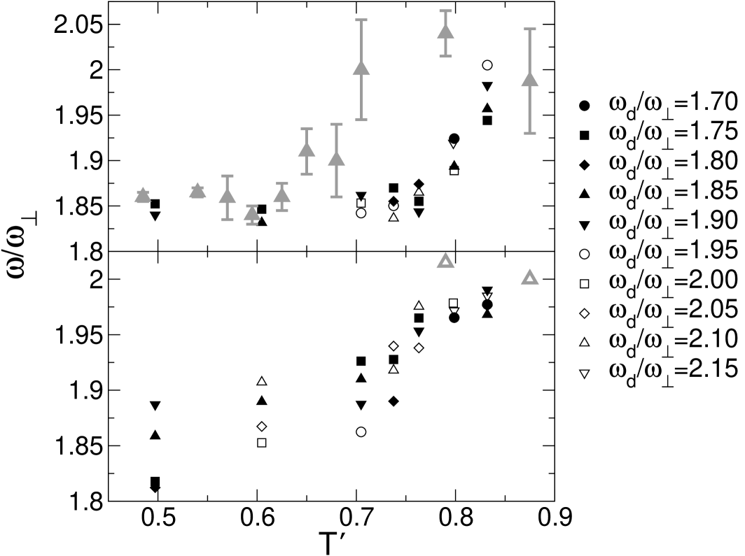
Figure 6: Condensate (upper frame) and the thermal cloud (lower frame) frequencies for the $m=0$ collective mode as a function of reduced temperature. Black (solid and open) symbols correspond to the numerical results obtained for various driving frequencies (according to the legend) whereas gray symbols (solid for the condensate and open for the thermal cloud) with error bars are taken from the experiment by Jin et al. Cornell-osc .

Our results also show that the notion of natural condensate frequency breaks down when the thermal cloud is present. The condensate response depends on the dynamics of the thermal cloud and, in fact, the possible frequencies for the condensate oscillation lie in an interval which gets wider for higher temperatures. In particular, no two branches of frequencies are visible as reported in Ref. Zaremba-osc . In Fig. 7 we compare the numerical and experimental damping rates for the oscillations of the condensed and noncondensed components. There is some discrepancy for higher temperatures where the thermal component seems to be damped too strongly in comparison with the experimental data. Perhaps this increases the temperature at which the frequency of the condensate fraction shifts up.

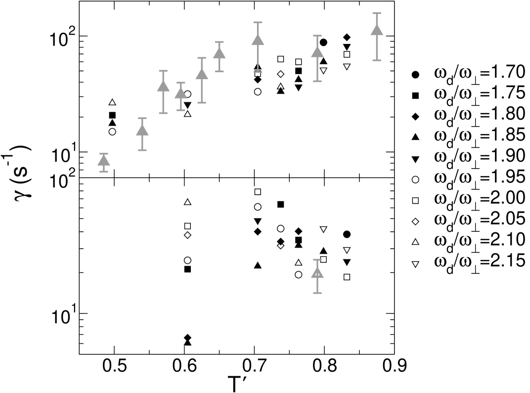
Figure 7: Damping rates for the condensate (upper frame) and the thermal cloud (lower frame) for the $m=0$ mode as a function of reduced temperature. Black (solid and open) symbols correspond to the numerical results obtained for various driving frequencies (according to the legend) whereas gray symbols (solid for the condensate and open for the thermal cloud) with error bars are taken from the experiment by Jin et al. Cornell-osc .

IV Results for the m=2 mode

We now do the same analysis for the $m=2$ mode. The system is disturbed by changing the trapping potential according to (22) with the phase shift $\phi=\pi$. Such a perturbation excites the quadrupole $m=2$ oscillations. The classical field is split into the condensed and thermal parts and the condensate and thermal widths are calculated using formulas exhibiting the $m=2$ mode’s symmetry:

$$w_{c,th}=\int dx\,dy\,(x^{2}-y^{2})\,n_{c,th}(x,y)\,.$$ (25)

As before, these data are fitted by exponentially damped sine waves.

Frequencies and damping rates for the condensate and the thermal cloud are plotted in Figs. 8 and 9. Again, the system responds in a way that depends on the driving frequency. A comment on how the authors of the experiment Cornell-osc choose the driving frequency is in place here. They say that the driving frequency is set to match the frequency of the excitation being studied. This could make sense for $m=0$ mode where supposedly the condensed and noncondensed fractions always oscillate in phase. Supposedly, because in Cornell-osc we see only two data points (both having frequency approximately $2\omega_{\bot}$) showing the behavior of the thermal cloud in the $m=0$ mode. However, for the $m=2$ mode the frequencies at which the condensate and thermal cloud oscillate are different, and the meaning of the driving frequency as the frequency of the excitation being studied is not clear. Therefore, in Fig. 8 we show our data for various driving frequencies. Good agreement with experiment is found for appropriate driving frequencies up to temperatures $\approx 0.8T_{c}$. For temperatures approaching the critical one, however, we observe the same effect as for the $m=0$ mode. The thermal cloud becomes dominant and the frequencies at which the condensate oscillates become higher. Fig. 8 shows that already for a temperature $T=0.83T_{c}$, with the driving frequency $\omega_{d}=1.75\omega_{\bot}$, the condensate oscillates with the frequency of the thermal cloud. Such a behavior was not observed experimentally. On the other hand, it is an expected behavior, since the condensed fraction becomes smaller and smaller while the critical temperature is approached, and the dynamics should be dominated by the thermal cloud. In the case of the thermal cloud, our model predicts frequencies in agreement with the experiment (other theoretical studies of the JILA experiment either do not show results for the thermal atoms for the $m=2$ mode, or predict frequencies that are very different than observed experimentally).

In Fig. 9 we compare the numerical and experimental damping rates for the oscillations of the condensed and noncondensed parts of the system. As for the $m=0$ mode, there is some discrepancy for higher temperatures where the thermal cloud is damped too strongly, whereas the condensate is damped too weakly.

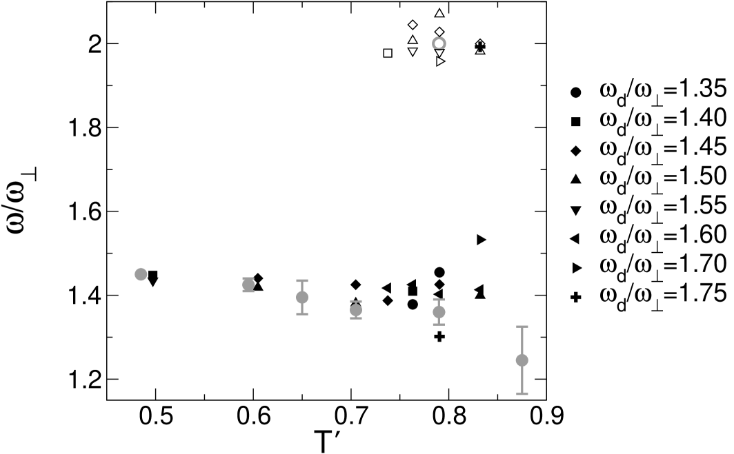
Figure 8: Condensate (solid symbols) and thermal cloud (open symbols) frequencies for the $m=2$ collective mode, as a function of reduced temperature. Black symbols correspond to the numerical results obtained for various driving frequencies (according to the legend, here the shape of the symbol determines the driving frequency), whereas gray symbols with error bars are taken from the experiment by Jin et al. Cornell-osc . Note, however, that the only experimental point for the thermal cloud is marked with an open gray circle.

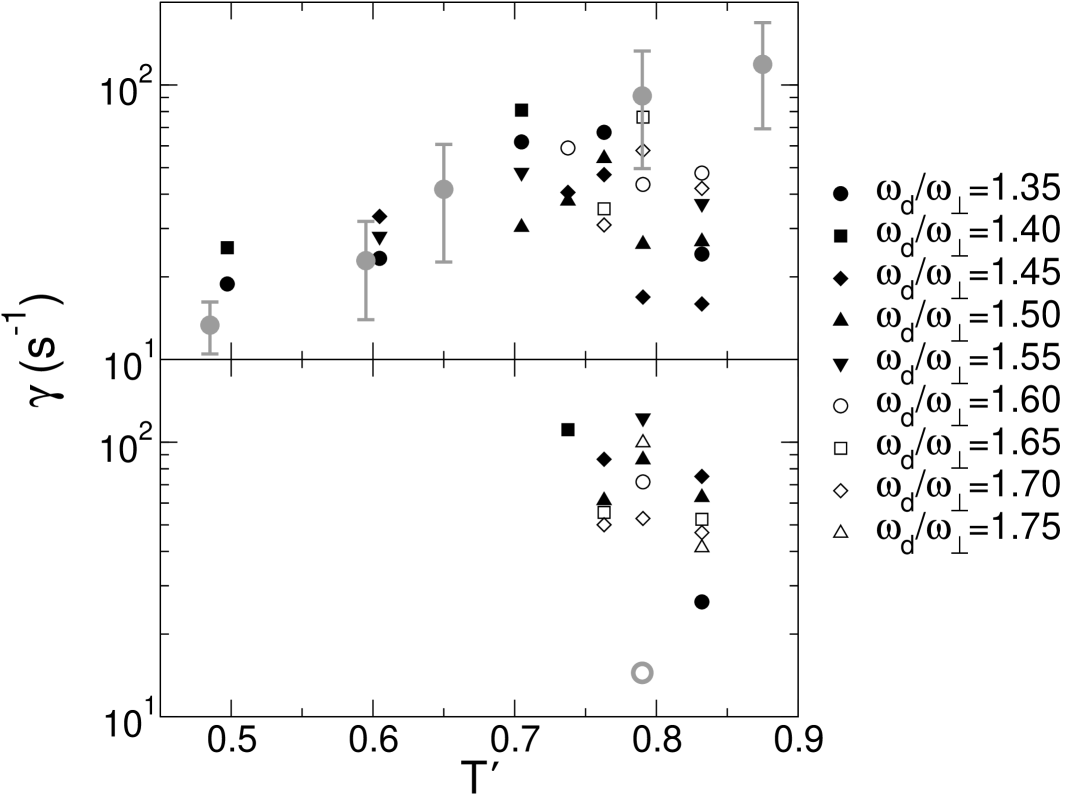
Figure 9: Damping rates for the condensate (upper frame) and the thermal cloud (lower frame) for the$m=2$ mode, as a function of reduced temperature. Black (solid and open) symbols correspond to the numerical results obtained for various driving frequencies (according to the legend), whereas gray symbols (solid for the condensate and open for the thermal cloud) with error bars are taken from the experiment by Jin et al. Cornell-osc . Note that the only experimental point for the thermal cloud is marked with an open gray circle.

V Conclusions

In conclusion, we have presented in detail the construction of the classical field describing the desired number of atoms, confined in any trapping potential, at a prescribed temperature. We have studied the oscillations of the Bose-Einstein condensate in the presence of a thermal cloud. As in the experiment, we find the temperature dependent condensate frequency shift for both the $m=0$ and $m=2$ collective oscillation modes. For the $m=0$ mode, the thermal atoms pull the condensate fraction along, and above some characteristic temperature $(\approx 0.8T_{c})$ the condensate tends to oscillate with the frequency of the thermal part (approximately equal to $2\omega_{\bot}$). Unfortunately, in the present version of the classical field approximation, the value of this characteristic temperature turns out to be about $20\%$ higher than the one observed in the experiment. For the $m=2$ mode, on the other hand, the frequency at which the condensate oscillates first decreases with an increase of temperature (the thermal cloud oscillating with its natural frequency equal to $2\omega_{\bot}$ damps the condensate motion) but when the temperature gets closer to the critical temperature the condensate starts to oscillate with higher frequencies, approaching the frequency of the thermal cloud.

- (1) D.S. Jin, J.R. Ensher, M.R. Matthews, C.E. Wieman, and E.A. Cornell, Phys. Rev. Lett. 77, 420 (1996).
- (2) M.-O. Mewes, M.R. Andrews, N.J. van Druten, D.M. Kurn, D.S. Durfee, C.G. Townsend, and W. Ketterle, Phys. Rev. Lett. 77, 988 (1996).
- (3) D.S. Jin, M.R. Matthews, J.R. Ensher, C.E. Wieman, and E.A. Cornell, Phys. Rev. Lett. 78, 764 (1997).
- (4) D.M. Stamper-Kurn, H.-J. Miesner, S. Inouye, M.R. Andrews, and W. Ketterle, Phys. Rev. Lett. 81, 500 (1998).
- (5) O. Maragó, G. Hechenblaikner, E. Hodby, and Ch. Foot, Phys. Rev. Lett. 86, 3938 (2001).
- (6) F. Chevy, V. Bretin, P. Rosenbusch, K.W. Madison, and J. Dalibard, Phys. Rev. Lett. 88, 250402 (2002).
- (7) M. Edwards, P.A. Ruprecht, K. Burnett, R. J. Dodd, and C.W. Clark, Phys. Rev. Lett. 77, 1671 (1996); S. Stringari, Phys. Rev. Lett. 77, 2360 (1996).
- (8) T. Nikuni, E. Zaremba, and A. Griffin, Phys. Rev. Lett. 83, 10 (1999); E. Zaremba, T. Nikuni, and A. Griffin, J. Low Temp. Phys. 116, 277 (1999).
- (9) B. Jackson and E. Zaremba, Phys. Rev. Lett. 88, 180402 (2002).
- (10) S.A. Morgan, M. Rusch, D.A.W. Hutchinson, and K. Burnett, Phys. Rev. Lett. 91, 250403 (2003).
- (11) S.A. Morgan, Phys. Rev. A 72, 043609 (2005).
- (12) A. Bezett and P.B. Blakie, Phys. Rev. A 79, 023602 (2009).
- (13) N.P. Proukakis and B. Jackson, J. Phys. B 41, 203002 (2007).
- (14) P.B. Blakie, A.S. Bradley, M.J. Davies, R.J. Ballagh, C.W. Gardiner, Adv. Phys. 57, 363 (2008).
- (15) M. Brewczyk, M. Gajda, and K. Rza̧żewski, J. Phys. B 40, R1 (2007).
- (16) K. Góral, M. Gajda, and K. Rza̧żewski, Phys. Rev. A 66, 051602(R) (2002).
- (17) M. Brewczyk, P. Borowski, M. Gajda, and K. Rza̧żewski, J. Phys. B 37, 2725 (2004).
- (18) K. Góral, M. Gajda, and K. Rza̧żewski, Phys. Rev. Lett. 86, 1397 (2001).
- (19) H. Schmidt, K. Góral, F. Floegel, M. Gajda, and K. Rza̧żewski, J. Opt. B 5, S96 (2003).
- (20) Ł. Zawitkowski, M. Gajda, and K. Rza̧żewski, Phys. Rev. A 74, 043601 (2006).
- (21) K. Gawryluk, M. Brewczyk, M. Gajda, and K. Rza̧żewski, Phys. Rev. A 76, 013616 (2007).
- (22) K. Gawryluk, M. Brewczyk, and K. Rza̧żewski, J. Phys. B 39, L225 (2006); K. Gawryluk, T. Karpiuk, M. Brewczyk, and K. Rza̧żewski, Phys. Rev. A 78, 025603 (2008).
- (23) N.N. Bogoliubov, J. Phys. Moscow 11, 231 (1947).
- (24) O. Penrose and L. Onsager, Phys. Rev. 104, 576 (1956).
- (25) T. Karpiuk, M. Brewczyk, M. Gajda, and K. Rza̧żewski, J. Phys. B 42, 095301 (2009).
- (26) A. Sinatra, C. Lobo, and Y. Castin, Phys. Rev. Lett. 87, 210404 (2001); A. Sinatra, C. Lobo, and Y. Castin, J. Phys. B 35, 3599 (2002).
- (27) E. Witkowska, M. Gajda, and K. Rza̧żewski, Phys. Rev. A 79, 033631 (2009).
- (28) C.J. Pethick and H. Smith, Bose-Einstein Condensation in Dilute Gases (Cambridge University Press, Cambridge, United Kingdom, 2002).
- (29) F. Gerbier, J.H. Thywissen, S. Richard, M. Hugbart, P. Bouyer, and A. Aspect, Phys. Rev. A 70, 013607 (2004).