Extending the Hubble diagram by gamma ray bursts
(Research Note)

Abstract

Aims. A new method to constrain the cosmological equation of state is proposed by using combined samples of gamma-ray bursts (GRBs) and supernovae (SNeIa).

Methods. The Chevallier-Polarski-Linder parameterization is adopted for the equation of state in order to find out a realistic approach to achieve the deceleration/acceleration transition phase of dark energy models.

Results. We find that GRBs, calibrated by SNeIa, could be good distance indicators capable of discriminating between cosmological models and $\Lambda$CDM model at high redshift.

1 Introduction

From an observational viewpoint, one of the fundamental goals of cosmology is to measure cosmological distances and then to build up a suitable and reliable cosmic distance ladder. This issue has recently become even more important due to the evident degeneracy of several dark energy models with $\Lambda$CDM, despite the advent of the so-called Precision cosmology, (Ellis, 1999).

In the last two decades, a class of accurate standard candles, the supernovae type Ia (SNeIa), has been highly studied and the results obtained from the use of these objects led to the surprising discovery of the acceleration of the cosmic Hubble flow (for a review see Kowalski et al 2008). However these objects are poorly detectable at redshifts higher than $\sim 1.5$, so we need distance indicators at higher redshifts in order to remove the degeneration of dark energy models affecting current cosmological models ($\Lambda$CDM is a good approximation of the observed Universe, even though there is still no theoretical basis about the nature of its components, but the issue of global evolution is far from being addressed; for a comprehensive review see Copeland et al 2006). A possible solution could be found by adopting gamma ray bursts (GRBs) as distance indicators.

GRBs are the most powerful explosions in the Universe: the most likely scenarios for their generation are the formation of massive black holes or the coalescence of binary stellar systems. These events are observed at considerable distances, so there have been several efforts to frame them into the standard of the cosmological distance ladder. In the literature, there are several models that account for GRB formation (Meszaros, 2006). All these scenarios involve a similar shock phenomenon: a ”fireball”, possibly be supported by a further jet emission. However none of these models is intrinsically capable of integrating all the observable quantities.

Despite the poor knowledge of the GRB mechanism, it seems that GRBs could be used as reliable distance indicators. There exist several observational correlations among the photometric and spectral properties of GRBs to support this possibility (Basilakos $\&$ Perivolaropoulos, 2008; Ghirlanda et al, 2006). Nevertheless the origin of these spectroscopic and photometrical correlations is not known very well and there are several efforts to interpret the behavior of GRB features in a coherent way, by relatively simple scenarios (Dainotti et al, 2008; Ghisellini et al, 2008). Succeeding in explain the mechanism that generates GRBs is one of the objectives of modern astrophysics and to clarify these observed correlations in this context would make GRBs reliable distance indicators. A complete review of the existing luminosity relations for GRBs can be found in Schaefer (2007).

In this paper, we consider two relations, the one by Liang-Zhang (LZ) (Liang $\&$ Zhang, 2005), and the one by Ghirlanda (GGL) (Ghirlanda et al, 2004). They are the only 3-parameter relations known and have less scatter with respect to the theoretical best fit than the other 2-parameter ones. However calibration of the relations used has been necessary in order to avoid the circularity problem. This means that all the relations need to be calibrated for each set of cosmological parameters. Indeed, all GRB distances, obtained in a photometric way, are strictly dependent on the cosmological parameters since, currently, there is no low-redshift ($z$ up to 0.2-0.3) set of GRBs available to achieve a cosmology-independent calibration. In order to overcome this difficulty, Liang et al. (2008), proposed a method in which several GRB relations have been calibrated by SNeIa. Supposing that these relations work at all redshifts and that, at the same redshift, GRBs and SNeIa have the same luminosity distance, it becomes possible, in principle, to calibrate the GRB relations using an interpolation algorithm. In this way, it becomes possible to build a GRB-Hubble diagram by calculating the luminosity distance for each GRB with the well-known relation between the luminosity distance $d_{l}$ and the energy-flux ratio of the distance indicators.

In the literature there are several paper that use similar methods to constraint the cosmological parameters of the Concordance Model using GRBs as extension of the SNeIa Hubble Diagram, (Firmani et al., 2005, 2006; Wang & Dai, 2006; Wang et al., 2007; Li et al., 2008, ).

Here we take into account a cosmological EoS working at any redshift, using GRBs as tracers and adopting again the Chevallier-Polarski-Linder (CPL) parameterization. In particular we discuss a method which should allow us to obtain an analytic cosmology-independent formulation of the luminosity distance and then of the distance modulus. After a brief introduction to the GRB luminosity relations, we show fits of the data obtained by these relations and the results and perspectives of the approach are discussed in the last Section.

2 The theoretical framework

Our goal is to obtain an analytic formulation of the Hubble diagram valid at any redshift. We start from the Friedmann equation

$$H^{2}=\frac{8\pi G}{3}\rho-\frac{kc^{2}}{a^{2}}\,.$$ (1)

We obtain, by some algebra, the following equation in terms of the density parameter

$$H^{2}=H_{0}^{2}\left[\Omega_{0}\left(\frac{a_{0}}{a}\right)^{3(w+1)}-\left(\Omega_{0}-1\right)\left(\frac{a_{0}}{a}\right)^{2}\right],$$ (2)

where the subscript $0$ indicates the present value of the parameters. From now onwards, we take into account a spatially quasi-flat Universe, $k\approx 0$; the contribution of the curvature will be negligible and we have $\Omega_{0}\approx 1$, as suggested by the latest CMBR (Komatsu et al, 2008) and the SNeIa observations (Kowalski et al, 2008). However, in the final section, we will perform a test to verify this assumption with observations coming from GRBs. Now if we translate in terms of redshift $z$,

$$\frac{a_{0}}{a}=1+z\,,$$ (3)

the previous equation reduces to

$$H^{2}(z)=H_{0}^{2}\left(1+z\right)^{3(w+1)}\,.$$ (4)

The $w$-parameter indicates the EoS $w=p/\rho$, where $p$ and $\rho$ are the pressure and the matter-energy density of the Universe, respectively. Considering the CPL parameterization of the EoS, (Chevallier et al, 2001):

$$w(z)=w_{0}+w_{a}\frac{z}{1+z},$$ (5)

and substituting into Eq.(4), we obtain:

$$H(z)=H_{0}\left[\left(1+z\right)^{\frac{3}{2}(w_{0}+w_{a}+1)}\exp{\left(\frac{-3w_{a}z}{2(1+z)}\right)}\right],$$ (6)

which enters directly in the expression of the distance modulus

$$\mu(z)=-5+5\log{d_{l}(z)}\,,$$ (7)

where $d_{l}(z)=c(1+z)D_{l}(z)$ and where

$$D_{l}(z)=\int_{0}^{z}\frac{d\xi}{H(\xi)}\,.$$ (8)

This means that an analytic expression for $\mu$ can be achieved. The integral $D_{l}$ in Eq.(8) can be solved giving a Gamma function of the first kind :

$$D_{l}(z)=\left(\frac{3w_{a}}{2}\right)^{-\frac{1+3w_{0}+3w_{a}}{2}}$$

$$\left.\exp{\left(\frac{3w_{a}}{2}\right)}\Gamma\left[\frac{1+3w_{0}+3w_{a}}{2},\frac{3w_{a}}{2(1+\xi)}\right]\right|_{\xi=0}^{\xi=z}.$$ (9)

Substituting such an expression in the distance modulus, we obtain a model for data fitting which could work, in principle, at any $z$. The obtained expression for the Hubble parameter $H(z)$ is independent of the density parameters, $\Omega_{M}$ and $\Omega_{\Lambda}$, provided that their sum is equal to 1.

We use the CPL parameterization not only for the dark energy component, but for the total energy-matter density of the Universe. This assumption works because dark and baryonic matter contribute with a null pressure while the radiation component is negligible in matter- and dark energy-dominated eras. Furthermore, the analytical formulation that we adopt for the luminosity distance is assumed valid at any redshift $z$.

3 GRB luminosity relations

In the last years, thanks to several spacecraft missions capable of observing this high energy region, the main features of GRBs have become better known. Recently, some photometric and spectroscopic relations between GRB observables have been found and then the hypothesis that these objects could be considered suitable distance indicators has become feasible. Nevertheless, there is no theoretical model that fully explains these relations so the GRBs cannot be considered as standard candles. For a detailed review of the observational features see Schaefer (2007).

Here, we take into account the existing 3-parameter relations. This choice has been made because these relations place better constraints on the data giving less scatter between the theoretical relation and the experimental data (Schaefer, 2007). The first relation is the so-called Liang-Zhang relation, (Liang $\&$ Zhang, 2005), which allows us to connect the GRB peak energy, $E_{p}$, with the isotropic energy released in the burst, $E_{iso}$, and with the jet break - time of the afterglow optical light curve in the rest frame, measured in days, $t_{b}$, that is

$$\log{E_{iso}}=a+b_{1}\log{\frac{E_{p}(1+z)}{300keV}}+b_{2}\log{\frac{t_{b}}{(1+z)1day}}$$ (10)

where $a$ and $b_{i}$, with $i=1,2$, are calibration constants.

The other relation is that given by Ghirlanda et al (Ghirlanda et al, 2004). It connects the peak energy $E_{p}$ with the collimation-corrected energy, or the energy release of a GRB jet, $E_{\gamma}$, where $E_{\gamma}=F_{beam}E_{iso}=1-\cos({\theta})E_{iso}$, with $\theta_{jet}$ the jet opening angle defined in Sari et al (1999):

$$\theta_{jet}=0.163\left(\frac{t_{b}}{1+z}\right)^{3/8}\left(\frac{n_{0}\eta_{\gamma}}{E_{iso,52}}\right)^{1/8},$$ (11)

where $E_{iso,52}=E_{iso}/10^{52}$ ergs, $n_{0}$ is the circumburst particle density in 1 cm^-3, and $\eta_{\gamma}$ the radiative efficiency. The Ghirlanda et al. relation is

$$\log{E_{\gamma}}=a+b\log{\frac{E_{p}}{300keV}},$$ (12)

where $a$ and $b$ are two calibration constants.

From these relations, we can directly obtain the luminosity distance $d_{l}$ from the well-known formula which connects $d_{l}$ with the isotropic energy $E_{iso}$ and the bolometric fluence $S_{bolo}$ :

$$d_{l}=\left(\frac{E_{iso}}{4\pi S_{bolo}}\right)^{\frac{1}{2}},$$ (13)

from which it is easy to compute, for each GRB, the distance modulus $\mu=$ and its error given by (Liang et al, 2008):

$$\sigma_{\mu}=\left[\left(2.5\sigma_{\log{E_{iso}}}\right)^{2}+\left(1.086\sigma_{S_{bolo}}/S_{bolo}\right)^{2}\right]^{\frac{1}{2}}$$ (14)

with $\sigma_{\log{E_{iso}}}$ and $\sigma_{S_{bolo}}$ obtained from the error propagation applied to Eq.(10) and Eq.(12). Moreover, we assume that the error in the determination of the redshift $z$ is negligible, as well as for the radiative efficiency $\eta_{\gamma}$. We note also that the assumption of a well-known $n_{0}$ is a strong hypothesis since the goodness of the fits depends, in particular, on this parameter. The GRB data sample is taken from the already cited work by Schaefer. We take into account 27 events with extremely precise data. This sample is the same one adopted in Capozziello $\&$ Izzo (2008).

4 The data fitting

The next step is the fit of the GRB sample with the empirical relations, Eqs.(10),(12), described in Sect. 3. The aim is to achieve an estimate of the CPL parameters and consequently to determine the trend of the EoS at any redshift, using the analytical relation, Eq.(2). We are considering the same sample of 27 GRBs used in Capozziello $\&$ Izzo (2008) in which we have added the sample of SNeIa by the Union Supernova Survey (Kowalski et al, 2008).

The numerical results of the fits are shown in Table 1, where we obtain a robust estimation of the CPL parameters for both the relations used, with and without SNeIa data. An immediate comparison is done with the best fit applied only to the SNeIa sample. It is evident how adding GRBs to SNeIa data completes the knowledge of and the accuracy on the EoS parameter $w$.

Table 1: Results of the fits. SNeIa is only for the supernovae data, LZ is for the GRBs data obtained from the Liang-Zhang relation, GGL for the Ghirlanda et al. one.

Relation	$w_{0}$	$w_{a}$	$R^{2}$
SNeIa	$-0.910\pm 0.070$	$0.755\pm 0.054$	$0.983$
LZ	$-1.39\pm 0.38$	$1.18\pm 0.37$	$0.817$
GGL	$-1.46\pm 0.38$	$1.36\pm 0.32$	$0.812$
LZ + SNeIa	$-1.15\pm 0.10$	$0.93\pm 0.11$	$0.933$
GGL + SNeIa	$-1.42\pm 0.12$	$1.24\pm 0.13$	$0.920$

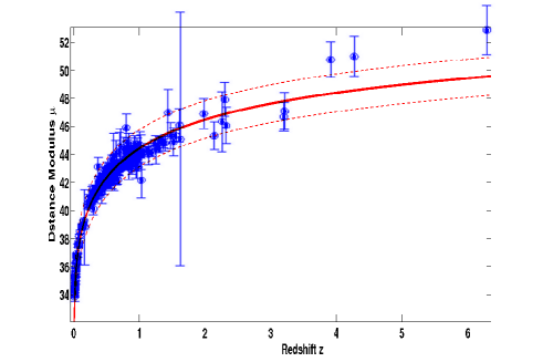
Figure 1: Redshift-distance modulus diagram for the GRB+SNeIa sample. The black dots are the GRBs , the blue ones are the SNeIa. The red line is the best fit obtained from the data, with the dashed line representing the confidence limits at $3\sigma$. The error bars on the supernova data are not represented because they are negligible.

In order to measure the goodness of the fit, we use the $R^{2}$ test, see Table 1. The $R^{2}$ test is a measure of how successful the fit is in explaining the variation of the data (see for details Draper $\&$ Smith 1998). An $R^{2}$ close to 1.0 indicates that we have accounted for almost all of the variability with the data specified in the model. As a standard, the $R^{2}$ test is the square of the correlation between the response values and the predicted response values, that is:

$$R^{2}=1-\frac{SSE}{SST}=1-\frac{\sum_{i=1}^{n}w_{i}(y_{i}-\hat{y}_{i})}{\sum_{i=1}^{n}w_{i}(y_{i}-\bar{y}_{i})^{2}},$$ (15)

where $SSE$ is the sum of the squares due to errors and it measures the total deviation of the response values from the fit and $SST$ is the sum of squares about the mean: $\hat{y}$ is the predicted response value, $\bar{y}$ is the mean value and the $w_{i}$ are the weights on the values.

The extension of the supernova Hubble Diagram with the GRB data can be used to improve our knowledge of the trend at high redshift. In this way, also using the GRB data, we show in Fig.  3, the distance modulus $\mu$ versus the redshift $z$, in a logarithmic scale. The best fit curve, obtained with Eq.(2), is also reported. A more detailed analysis confirms the presence of a transition (re-acceleration) redshift around $z=0.5$.

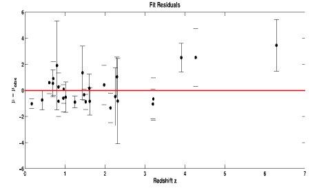
Figure 2: Comparison between the best fit of $\mu$ and the observed distance modulus $\mu_{obs}$ at any redshift. The black dots are the GRBs data and the red line is the best fit curve representing the theoretical distance modulus.

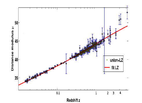
Figure 3: Redshift-distance modulus diagram for the GRB+SNeIa sample versus redshift in logarithmic scale.

In Fig.  2, we plot the comparison between the theoretical $\mu_{th}$ and the observed distance modulus $\mu_{obs}$ at any redshift, the residual plot. A smooth trend up to $z\approx 3.5$ in the residual curve can be immediately detected. Beyond this limit, we have 3 GRBs that exceed, by the same side, the $3\sigma$ confidence limit of the best fit. This discrepancy is clear in Fig.  3, where we plot the best fit for the combined sample in the case of an LZ relation with a logarithmic scale for the redshift.

This fact is fundamental for the goodness of the fit because these GRBs represent the most distant objects that one can use to make such an analysis and their weight on the fit is very high, in the sense that they appear to be not accurate distance indicators.

However there is strong evidence that the data of these 3 GRBs, GRB 050505, GRB 050904 and GRB 060210, reported in the Schaefer catalog, are uncertain. For the first and the last GRB the peak energies are underestimated (Cabrera et al., 2007). As a consequence we would obtain an underestimated value for the bolometric fluence. GRB 050904 is the most distant GRB considered and it shows some probelms related to the peak energy reported by different authors, that differ by a factor of $\sim 3$. Moreover the afterglow of GRB is complicated by flares and re-brightenings so that the standard afterglow model gives an extremely high value of the circumburst medium density $n\sim 700cm^{-3}$ (Frail et al., 2006), contrary to the assumed value $n=3cm^{-2}$.

For this reason we repeat the analysis described above without these 3 GRBs, obtaining a better value than the previous one for the $R^{2}$ test. The results of these corrected fits are shown in Table 3. In Fig.  4, we plot the best fit with this corrected sample. From these results we conclude that the complete sample gives different results than does corrected sample, the first one suggesting a phantom/quintessence regime for the present epoch while the second one fits an accelerating $\Lambda$CDM model. This last result is confirmed by the following analysis, where we have performed a Monte-Carlo-like procedure for the comparison of the results with the usual likelihood estimator given by

$$\chi^{2}=\sum_{i=1}^{N}\left[\frac{(\mu_{th}(z_{i})-\mu_{obs}(z_{i}))^{2}}{\sigma_{i}}\right],$$ (16)

in the context of a $\Lambda$CDM model of the Universe, where $\mu_{th}$ is the distance modulus computed from the Eq.(7) and Eq.(8), $z_{i}$ is the observed redshift for each GRB and $\sigma_{i}$ the observed distance modulus uncertainty. The results of this analysis are shown in Table 2, where we can see the improvement obtained by the GRB sample corrected for the 3 ”wrong” GRBs.

We have adopted a similar procedure in the case of an EoS evolving with redshift and where $\mu_{th}$ is obtained by Eq.(2). The result of this analysis is plotted in Fig.  5 where the best fit value, the cross in the figure, corresponds to the value $w_{0}=-0.84\pm 0.14$ and $w_{a}=0.72\pm 0.06$, and where the boundaries correspond to 1$\sigma$, 2$\sigma$ and 3$\sigma$ confidence levels, in a good agreement with the results obtained, see Table 3, using our theoretical relation, Eq.(2).

From this analysis, we conclude that the corrected sample agrees fairly well with the $\Lambda$CDM model with a small contribution of the curvature parameter, $k=0.01\pm 0.04$. Thus, the method delineated in Sect.2 seems a good approximation of the observed cosmography and agrees very well with the $\Lambda$CDM model, so that we can argue that GRBs could be good distance indicators at redshift values up to $z=4$.

Table 2: Cosmological density parameters, with uncertainties computed at 1$\sigma$ confidence limit, obtained by a Monte Carlo procedure

Sample	$\Omega_{m}$	$\Omega_{\Lambda}$	$\Omega_{k}$	$\chi^{2}$
UNION + GRB	$0.26\pm 0.14$	$0.73\pm 0.14$	$0.01\pm 0.04$	$1.032$
UNION + GRB corrected	$0.25\pm 0.10$	$0.74\pm 0.135$	$0.01\pm 0.035$	$1.00027$

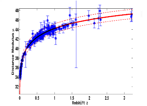
Figure 4: Redshift-distance modulus diagram for the corrected GRB+SNeIa sample. The red line is the best fit obtained from the data, with the dashed line representing the confidence limit at $3\sigma$.

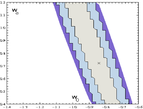
Figure 5: 68%, 95% and 98% constraints on $w_{0}$ and $w_{a}$ obtained from the UNION sample and the GRB sample corrected for the 3 outlying GRBs. The cross represents the best fit value and it is in a good agreement with that found using the theoretical model described in Sect.2.

5 Discussion and conclusions

Starting from the Friedmann equation, we have investigated a new method to constrain the cosmological equation of state at high redshifts. In particular we obtain an analytical formula for the distance modulus so we could directly estimate the parameters of the cosmological model considered. The working hypothesis involves the use of GRBs as distance indicators at high redshift, well beyond the distance where SNeIa have been detected to date. The CPL parameterization for the EoS has been explicitly used for the whole matter-energy content of the Universe as a suitable approach to investigate the parameter $w=w(z)$ and discriminate values with respect to the $\Lambda$CDM model. In particular, regarding the Friedmann equations, we have obtained, in the case of the LZ relation, the epoch for the transition between the deceleration-acceleration phases at a redshift value of $z\approx 5$, with a reliable confidence level. This is a value that, if higher than the redshift of the farthest GRB used, could be in agreement with current quasar formation scenarios. Also, we are in good agreement with the observed phantom/quintessence regime at the present epoch, that is for $z\rightarrow 0$, we obtain $w\leq-1$.

So we reject the current phantom regime by this analysis, obtaining for $w_{0}$ a value in agreement with the $\Lambda$CDM model at the present epoch. The method, while preliminary, seems to indicate that GRBs could be used as standard candles once a reliable unified model of their photometric and spectroscopic quantities is achieved (some relevant results are presented in Ghisellini et al 2008). However, more robust samples of data are needed and a more realistic EoS (with respect to the simple perfect fluid models) should be taken into account in order to suitably track redshift at any epoch (see for example Capozziello et al 2006).

With improving observations, in particular with the launch of new satellites devoted to GRB surveys, such as Fermi-GLAST and AGILE, one should be able to expand the samples of GRBs, possibly with data coming from objects at higher redshift.

Considering these preliminary results, it seems that GRBs could be considered as a useful tool to remove degeneracy and constrain self-consistent cosmological models. The matching with other distance indicators would improve the consistency of the Hubble distance-redshift diagram by extending it up to redshift $6\,-\,7$ and higher.

Table 3: Results of the fits corrected for the 3 “outying” GRBs. SNeIa is for the supernova Ia data, LZ is for the GRBs data obtained from the Liang-Zhang relation, GGL for the Ghirlanda et al. one.

Relation	$w_{0}$	$w_{a}$	$R^{2}$
LZ + SNeIa	$-0.95\pm 0.01$	$0.74\pm 0.01$	$0.999$
GGL + SNeIa	$-0.865\pm 0.005$	$0.66\pm 0.005$	$0.999$

References

- Albrecht et al (2006) Albrecht, A., et al, 2006, arXiv:astro-ph/0609591
- Basilakos Perivolaropoulos (2008) Basilakos, S., Perivolaropoulos, L., 2008, MNRAS, 391, 411
- Branch Tammann (1992) Branch, D., Tammann, G. A., 1992, Ann. Rev. Astron. Astrophys., 30, 359
- Cabrera et al. (2007) Cabrera, J. I., et al., 2007, MNRAS, 382, 342
- Capozziello et al. (2006) Capozziello, S., V.F. Cardone, V.F., Elizalde, E., Nojiri, S., Odintsov, S.D., 2006, Phys. Rev. D 73, 043512
- Capozziello Izzo (2008) Capozziello, S., Izzo, L., 2008, AA, 490, 31
- Capozziello et al. (2008) Capozziello, S., Cardone, V.F., Salzano, V. 2008, Phys. Rev. D 78, 063504.
- Chevallier et al (2001) Chevallier, M., Polarski, D., 2001, Int. J. Mod. Phys. D., 10, 213; Linder, E. V., 2003, Phys. Rev. Lett., 90 091301
- Copeland et al (2006) Copeland, E.J., Sami, M., Tsujikawa, S., 2006, Int. J. Mod. Phys. D., 15, 1753.
- Dainotti et al (2008) Dainotti, M.G., Cardone, V.F., Capozziello, S., 2008, MNRAS, 391, L79
- Djorgovski et al. (1999) Djorgovski, S. G., Kulkarni, S. R., Bloom, J. S., Frail, D., Chaffee, F., Goodrich, R. 1999b, GCN Circ. 189, http://gcn.gsfc.nasa.gov/gcn /gcn3/189 .gcn3
- Draper Smith (1998) Draper, N.R. Smith, H., 1998, Applied Regression Analysis (Wiley, New York).
- Ellis (1999) Ellis, R., 1999, Phys. World, 6, 19
- Firmani et al. (2005) Firmani, C., et al., 2005, MNRAS, 360, L1
- Firmani et al. (2006) Firmani, C., et al., 2006, MNRAS, 372, L28
- Frail et al. (2006) Frail, D. A., et al., 2006, ApJL, 646, 99
- Ghirlanda et al (2004) Ghirlanda, G., Ghisellini, G., & Lazzati, D., 2004, ApJ, 616, 331
- Ghirlanda et al (2006) Ghirlanda, G., Ghisellini, G., & Firmani, C., 2006, New Journal of Physics, 8, 123
- Ghisellini et al (2008) Ghisellini, G., et al., 2008, arXiv: 0811.1038 [astro - ph]
- Israel et al. (1999) Israel, G., et al. 1999, AA, 348, L5
- Jimenez et al. (2001) Jimenez, R., Band, D., Piran, T., 2001, ApJ, 561, 171
- Komatsu et al (2008) Komatsu, E., et al, 2008, arXiv: astro-ph/0803.0547
- Kowalski et al (2008) Kowalski, M., et al, 2008, ApJ, 686, 749
- Kulkarni et al. (1999) Kulkarni, S. R. et al., 1999, Nature, 398, 389
- (25) Li, H. et al., 2008, Apj, 680, 92
- Li et al. (2008) Li, H. et al., 2008, PhLB, 658, 95
- Liang et al (2008) Liang, N., et al, 2008, ApJ, 685, 354
- Liang Zhang (2005) Liang, E., & Zhang, B., 2005, ApJ, 633, 611
- Meszaros (2006) Meszaros, P., 2006, Rept. Prog. Phys., 69 2259
- Metzger et al. (1997) Metzger, M. R., Djorgovski, S. G., Kulkarni, S. R., Steidel, C. C., Adelberger, K. L., Frail, D. A., Costa, E., Frontera, F. 1997, Nature, 387, 878
- Riess et al. (1998) Riess, A. G., et al., 1998, ApJ, 116, 1009
- Rowan-Robinson (1985) Rowan-Robinson, M., 1985, The Cosmological Distance Scale (Freeman & co., New York)
- Sari et al. (1999) Sari, R., Piran, T., Halpern, J. P., 1999, ApJ, 519, L17
- Schaefer (2007) Schaefer, B. E., 2007, ApJ, 660, 16
- Visser (2004) Visser, M., 2004, Class. Quant. Grav., 21, 2603
- (36) Visser, M., Catton, C., 2007b, arXiv: gr-qc/0703122
- Wang & Dai (2006) Wang, F. Y., and Dai, Z. G., 2006, MNRAS, 368, 371
- Wang et al. (2007) Wang, F. Y., Dai, Z. G., and Zhu, Z. H., 2007, ApJ, 667, 1
- Weinberg (1972) Weinberg, S., 1972, Gravitation and Cosmology: Principles and applications of the general theory of relativity , (Wiley, New York)