Quantum properties of the three-mode squeezed operator: triply concurrent parametric amplifiers

Abstract

In this paper, we study the quantum properties of the three-mode squeezed operator. This operator is constructed from the optical parametric oscillator based on the three concurrent $\chi^{(2)}$ nonlinearities. We give a complete treatment for this operator including the symmetric and asymmetric nonlinearities cases. The action of the operator on the number and coherent states are studied in the framework of squeezing, second-order correlation function, Cauchy-Schwartz inequality and single-mode quasiprobability function. The nonclassical effects are remarkable in all these quantities. We show that the nonclassical effects generated by the asymmetric case–for certain values of the system parameters–are greater than those of the symmetric one. This reflects the important role for the asymmetry in the system. Moreover, the system can generate different types of the Schrödinger-cat states.

I Introduction

Squeezed light fulfils the uncertainty relation and has less noise than the coherent light in the one of the field quadratures. With the development of quantum information, squeezed states have become very important tool in providing efficient techniques for the encoding and decoding processes in the quantum cryptography hill . For instance, the two-mode squeezed states are of great interest in the framework of continuous-variable protocol (CVP) Ekert . In the CVP the quantum key distribution goes as follows. The two-mode squeezed source–such as parametric down conversion–emits two fields: one is distributed to Alice (A) and the other to Bob (B). Alice and Bob randomly choose to measure one of two conjugate field quadrature amplitudes. The correlation between the results of the same quadrature measurements on Alice’s and Bob’s side increases by increasing the values of the squeezing parameter. Through a public classical channel the users communicate their choices for the measurements. They keep only the results when both of them measure the same quadrature and hence the key is generated.

The generation of the multiparities squeezed entangled states is an essential issue in the multiparty communication including a quantum teleportation network van1 , telecloning van2 , and controlled dense coding van3 . The $N$-mode CV entangled states have been generated by combining $N$ single-mode squeezed light in appropriately coupled beam splitters van1 . The three-mode CV entangled states have taken much interest in the literatures, e.g., guo ; olsen ; fister ; van1 ; hua . For instance, it has been theoretically shown that tripartite entanglement with different wavelengths can be generated by cascaded nonlinear interaction in an optical parametric oscillator cavity with parametric down conversion and sum-frequency generation guo . Also, the three-mode CV states have been generated by three concurrent $\chi^{(2)}$ nonlinearities olsen . This has been experimentally verified by the observation of the triply coincident nonlinearities in periodically poled $KTiOPO_{4}$ fister . More details about this issue will be given in the next section. Furthermore, the comparison between the tripartite entanglement in the three concurrent nonlinearities and in the three independent squeezed states mixed on the beam splitters van1 , in the framework of the van Loock-Furusawa inequalities Furusawa , has been performed in olsen . It is worth mentioning that the generation of macroscopic and spatially separated three-mode entangled light for triply coupled $\chi^{(3)}$ Kerr coupler inside a pumped optical cavity has been discussed in hua . It has been shown that the bright three-mode squeezing and full inseparable entanglement can be established inside and outside the cavity.

Since the early days of the quantum optics squeezing is connected with what is so called squeezed operator. There have been different forms of this operator in the literatures, e.g. single ; two ; abdalla ; hon ; faisal ; barry ; marce . For example, degenerate and non-degenerate parametric amplifiers are sources of the single-mode single and the two-mode two squeezing, respectively. The quantum properties of the three-mode squeezed operator (TMS), which is constructed from two parametric amplifiers and one frequency converter, have been demonstrated in faisal . This operator can be represented by the $SU(1,1)$ Lie algebra generators faisal ; barry . Additionally, it can be generated–under certain condition–from bulk nonlinear crystal in which three dynamical modes are injected by three beams. Another possibility for the realization is the nonlinear directional coupler which is composed of two optical waveguides fabricated from some nonlinear material described by the quadratic susceptibility $\chi^{(2)}$. Finally, the mathematical treatments for particular type of the $n$-mode squeezed operator against vacuum states are given in hon .

In this paper, we treat the three concurrent parametric amplifiers given in olsen ; fister as three-mode squeezed operator. We quantitatively investigate the nonclassical effects associated with this operator when acting on the three-mode coherent and number states. For these states we investigate squeezing, second-order correlation function, Cauchy-Schwartz inequality and single-mode quasiprobability functions. This investigation includes the symmetric (equal nonlinearities) and asymmetric (non-equal nonlinearities) cases. In the previous studies the entanglement of the symmetric case only has been discussed olsen ; fister . The investigation in the current paper is motivated by the importance of the three concurrent parametric amplifiers in the quantum information research olsen ; fister ; van1 . Additionally, quantifying the nonclassical effects in the quantum systems is of fundamental interest in its own right. We prepare the paper in the following order. In section 2 we construct the operator and write down its Bogoliubov transformations. In sections 3 and 4 we study the quadrature squeezing, the second-order correlation function as well as the Cauchy-Schwartz inequality, respectively. In section 5 we investigate the single-mode quasiprobability functions. The main results are summarized in section 6.

II Operator formalism

In this section we present the operator formalism for the optical parametric oscillator based on the three concurrent $\chi^{(2)}$ nonlinearities. We follow the technique given in olsen ; fister to construct the Hamiltonian of the system. In this regard, we consider three modes injected into a nonlinear crystal, whose susceptibility is $\chi^{(2)}$, to form three output beams at frequencies $\omega_{0},\omega_{1},\omega_{2}$. The interactions are selected to couple distinct polarizations. Assuming that $x$ is the axis of the propagation within the crystal. The mode $\hat{b}_{1}$ is pumped at frequency and polarization $(\omega_{0}+\omega_{1},y)$ to produce the modes $\hat{a}_{1}(\omega_{0},z)$ and $\hat{a}_{2}(\omega_{1},y)$. The mode $\hat{b}_{2}$ is pumped at $(\omega_{1}+\omega_{2},y)$ to produce the modes $\hat{a}_{2}$ and $\hat{a}_{3}(\omega_{2},z)$. Eventually, the mode $\hat{b}_{3}$ is pumped at $(2\omega_{1},z)$ to produce the modes $\hat{a}_{1}$ and $\hat{a}_{2}$. The scheme for this interaction can be found in olsen ; fister . The interaction Hamiltonian for this concurrent triple nonlinearity takes the form olsen ; fister :

$$\hat{H}_{int}=i\hbar(\chi_{1}\hat{b}_{1}\hat{a}_{1}^{\dagger}\hat{a}_{2}^{\dagger}+\chi_{2}\hat{b}_{2}\hat{a}_{1}^{\dagger}\hat{a}_{3}^{\dagger}+\chi_{3}\hat{b}_{3}\hat{a}_{2}^{\dagger}\hat{a}_{3}^{\dagger})+{\rm h.c.},$$ (1)

where $\chi_{j},j=1,2,3,$ represent the effective nonlinearities and h.c. stands for the hermitian conjugate. The unitary operator associated with (1) is:

$$\hat{U}(t)=\exp\left(-it\frac{\hat{H}_{int}}{\hbar}\right).$$ (2)

In the undepleted pump approximation we set $r_{j}=\chi_{j}\langle\hat{b}_{j}(0)\rangle$ as real parameters. Now we obtain the requested squeezed operator as:

$$\hat{S}(\underline{r})=\exp[r_{1}(\hat{a}_{1}\hat{a}_{2}-\hat{a}_{1}^{\dagger}\hat{a}_{2}^{\dagger})+r_{2}(\hat{a}_{1}\hat{a}_{3}-\hat{a}_{1}^{\dagger}\hat{a}_{3}^{\dagger})+r_{3}(\hat{a}_{2}\hat{a}_{3}-\hat{a}_{2}^{\dagger}\hat{a}_{3}^{\dagger})],$$ (3)

where $(\underline{r})=(r_{1},r_{2},r_{3})$. Throughout this paper, the symmetric case means $r_{1}=r_{2}=r_{3}=r$, otherwise we have an asymmetric case. It is evident that three disentangled state can be entangled under the action of this operator. This operator provides the following Bogoliubov transformations:

$$\hat{S}^{\dagger}(\underline{r})\hat{a}_{j}\hat{S}(\underline{r})=f_{1}^{(j)}\hat{a}_{1}+f_{2}^{(j)}\hat{a}^{\dagger}_{1}+g_{1}^{(j)}\hat{a}_{2}+g_{2}^{(j)}\hat{a}^{\dagger}_{2}+h_{1}^{(j)}\hat{a}_{3}+h_{2}^{(j)}\hat{a}^{\dagger}_{3},\quad j=1,2,3$$ (4)

where $f^{(j)}_{j^{\prime}},g^{(j)}_{j^{\prime}},h^{(j)}_{j^{\prime}},j^{\prime}=1,2$ are functions in term of the parameters $r_{1},r_{2},r_{3}$. The formulae of these functions for the asymmetric case are rather lengthy. Nevertheless, we write down only here the explicit forms for the symmetric case as olsen :

$$\begin{array}[]{lr}f_{1}^{(1)}=\frac{1}{3}[2\cosh(r)+\cosh(2r)],\quad f_{2}^{(1)}=\frac{1}{3}[2\sinh(r)-\sinh(2r)],\\ g_{1}^{(1)}=\frac{1}{3}[-\cosh(r)+\cosh(2r)],\quad g_{2}^{(1)}=-\frac{1}{3}[\sinh(r)+\sinh(2r)],\\ g_{1}^{(1)}=h_{1}^{(1)}=f_{1}^{(2)}=h_{1}^{(2)}=f_{1}^{(3)}=g_{1}^{(3)},\\ f_{1}^{(1)}=g_{1}^{(2)}=h_{1}^{(3)},\quad f_{2}^{(1)}=g_{2}^{(2)}=h_{2}^{(3)},\\ g_{2}^{(1)}=h_{2}^{(1)}=f_{2}^{(2)}=h_{2}^{(2)}=f_{2}^{(3)}=g_{2}^{(3)}.\end{array}$$ (10)

Relations (4) and (10) will be frequently used in the paper. For the symmetric case, the entanglement has been already studied in terms of the van Loock-Furusawa measure olsen . It has been shown that the larger the value of $r$, the greater the quantity of the entanglement in the tripartite. Moreover, the tripartite CV entangled state created tends towards GHZ state in the limit of infinite squeezing, but is analogous to a W state for finite squeezing pati . In this paper we give an investigation for the entanglement of the asymmetric case from different point of view. This is based on the fact that the entanglement between different components in the system is a direct consequence of the occurrence of the nonclassical effects in their compound quantities and vice versa. We show that the asymmetric case can provide amounts of the nonclassical effects and/or entanglement greater than those of the symmetric case. Thus the asymmetry in the triply concurrent parametric amplifiers is important.

The investigation of the operator (3) will be given through the three-mode squeezed coherent and number states having the forms:

$$|\psi_{n}\rangle=\hat{S}(\underline{r})|n_{1},n_{2},n_{3}\rangle,\quad|\psi_{c}\rangle=\hat{S}(\underline{r})|\alpha_{1},\alpha_{2},\alpha_{3}\rangle.$$ (11)

Three-mode squeezed vacuum states can be obtained by simply setting $n_{j}=0$ or $\alpha_{j}=0$ in the above expressions. In the following sections we study the quantum properties for the states (11) in greater details.

III Quadrature Squeezing

Squeezing is an important phenomenon in the quantum theory, which can reflect the correlation in the compound systems very well. Precisely, squeezing can occur in combination of the quantum mechanical systems even if the single systems are not themselves squeezed. In this regard the nonclassicality of the system is a direct consequence of the entanglement. Squeezed light can be measured by the homodyne detector, in which the signal is superimposed on a strong coherent beam of the local oscillator. Additionally, squeezing has many applications in various areas, e.g., in quantum optics, optics communication, quantum information theory, etc [21] . Thus investigating squeezing for the quantum mechanical systems is an essential subject in the quantum theory. In this section we demonstrate different types of squeezing for the three-mode squeezed vacuum states (11). To do so we define two quadratures $\hat{X}$ and $\hat{Y}$, which denote the real (electric) and imaginary (magnetic) parts, respectively, of the radiation field as:

$$\begin{array}[]{lr}\hat{X}=\frac{1}{2}[\hat{a}_{1}+\hat{a}^{\dagger}_{1}+c_{1}(\hat{a}_{2}+\hat{a}^{\dagger}_{2})+c_{2}(\hat{a}_{3}+\hat{a}^{\dagger}_{3})],\\ \hat{Y}=\frac{1}{2i}[\hat{a}_{1}-\hat{a}^{\dagger}_{1}+c_{1}(\hat{a}_{2}-\hat{a}^{\dagger}_{2})+c_{2}(\hat{a}_{3}-\hat{a}^{\dagger}_{3})],\end{array}$$ (12)

where $c_{1},c_{2}$ are $c$-numbers take the values $0$ or $1$ to yield single-mode, two-mode and three-mode squeezing. These two operators, $\hat{X}$ and $\hat{Y}$, satisfy the following commutation relation:

$$[\hat{X},\hat{Y}]=iC,$$ (13)

where $C=(1+c_{1}^{2}+c_{2}^{2})/2$. It is said that the system is able to generate squeezing in the $x$- or $y$-quadrature if

$$S_{x} = \frac{2\langle(\Delta\hat{X})^{2}\rangle-C}{C}<0,$$ (14)

$${\rm or}$$

$$S_{y} = \frac{2\langle(\Delta\hat{Y})^{2}\rangle-C}{C}<0,$$

where $\langle(\Delta\hat{X})^{2}\rangle=\langle\hat{X}^{2}\rangle-\langle\hat{X}\rangle^{2}$ is the variance. Maximum squeezing occurs when $S_{x}=-1$ or $S_{y}=-1$.

For the symmetric case, one can easily deduce the following expressions:

$$\begin{array}[]{lr}S_{x}=\frac{1}{3(1+c_{1}^{2}+c_{2}^{2})}\{(1+c_{1}^{2}+c_{2}^{2})[2\exp(2r)+\exp(-4r)-3]+2(c_{1}+c_{2}+c_{1}c_{2})[\exp(-4r)-\exp(2r)]\},\\ \\ S_{y}=\frac{1}{3(1+c_{1}^{2}+c_{2}^{2})}\{(1+c_{1}^{2}+c_{2}^{2})[2\exp(-2r)+\exp(4r)-3]+2(c_{1}+c_{2}+c_{1}c_{2})[\exp(4r)-\exp(-2r)]\}.\end{array}$$ (18)

For the single-mode case, $c_{1}=c_{2}=0$, the expressions (18) reduce to:

$$\begin{array}[]{lr}S_{x}=\frac{1}{3}[2\exp(2r)+\exp(-4r)-3],\\ S_{y}=\frac{1}{3}[2\exp(-2r)+\exp(4r)-3].\end{array}$$ (21)

It is evident that the system cannot generate single-mode squeezing. This fact is valid for the asymmetric case, too. For the two-mode case, $c_{1}=1,c_{2}=0$, i.e. first-second mode squeezing, we obtain

$$\begin{array}[]{lr}S_{x}=\frac{1}{3}[\exp(2r)+2\exp(-4r)-3],\\ S_{y}=\frac{1}{3}[\exp(-2r)+2\exp(4r)-3].\end{array}$$ (22)

Squeezing can be generated in the $x$-component only with a maximum value at $r=\ln(2)/3$. Also the maximum squeezing, i.e. $S_{x}=-1$, cannot be established in this case. This is in contrast with the two-mode squeezed operator two for which $S_{x}=-1$ for large $r$. Roughly speaking, the quantum correlation in this system decreases the squeezing, which can be involved in the one of the bipartites. Finally, for three-mode case, $c_{1}=c_{2}=1$, we have

$$S_{x}=\exp(-4r)-1,\quad S_{y}=\exp(4r)-1.$$ (23)

Squeezing can be generated in the $x$-component only for $r>0$. Squeezing reaches its maximum value for large values of $r$. The origin of the occurrence squeezing in (23) is in the strong correlation among the components of the system. Moreover, the amount of the produced squeezing is two (four) times greater than that of the two-mode two (single-mode single ) squeezed operator for certain values of $r$.

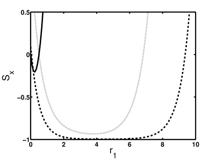
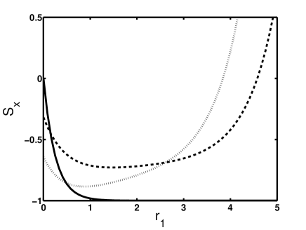
Figure 1: Two-mode (a) and three-mode (b) squeezing against $r_{1}$ for three-mode squeezed vacuum states. Solid, dashed and dotted curves are given for $(r_{2},r_{3})=(r_{1},r_{1}),(0.1,0.2)$ and $(0.4,0.6)$, respectively.

In Figs. 1(a) and (b) we plot the squeezing parameter $S_{x}$ against $r_{1}$ for two- and three-mode squeezing, respectively. We found that squeezing is not remarkable in $S_{y}$. The solid curve is plotted for the symmetric case. The two-mode squeezing is given for the first-second mode system. We start the discussion with the two-mode case (Fig. 1(a)). From the solid curve, squeezing is gradually generated as $r_{1}$ increases providing its maximum value $S_{x}=-0.206$ at $r=\ln(2)/3=0.231$, then it reduces smoothly and eventually vanishes, i.e. $S_{x}\geq 0$, at $r\geq\ln(1+\sqrt{3})/2=0.5025$. For the asymmetric case, squeezing increases gradually to be maximum $S_{x}=-1$ over a certain range of $r_{1}$, then rapidly decreases and vanishes (see the dashed and dotted curves). This can be understood as follows. When the values of $r_{2}$ and $r_{3}$ are relatively small, the main contribution in the system is related to the first parametric amplifier. Thus the system behaves as the conventional two-mode squeezed operator for a certain range of $r_{1}$. This remark is noticeable when we compare the dotted curve to the dashed one. Generally, when the values of $r_{2}$ and $r_{3}$ increase, the degradation of the squeezing increases, too. Furthermore, in the range of $r_{1}$ for which $S_{x}=-1$, the entanglement in the bipartite $(1,2)$ is maximum, however, this is not the case for the other bipartities. This is connected with the fact: the quantum entanglement cannot be equally distributed among many different objects in the system. Comparison among different curves in Fig. 1(a) shows that the asymmetric case can provide amounts of squeezing much greater than those of the symmetric case. Now, we draw the attention to the three-mode squeezing, which is displayed in Fig. 1(b). For the symmetric case, $S_{x}$ exhibits squeezing for $r>0$, which monotonically increases providing maximum value for large $r_{1}$, as we discussed above. This is in a good agreement with the fact that the symmetric case exhibits genuine tripartite entanglement for large values of $r_{1}$ cont . For the asymmetric case, the curves show initially squeezing, which reaches its maximum by increasing $r_{1}$, then it gradually decreases and vanishes for large values of $r_{1}$. The greater the values of $r_{2},r_{3}$ the higher the values of the maximum squeezing in $S_{x}$ and the shorter the range of $r_{1}$ over which squeezing occurs (compare dotted and dashed curves in Fig. 1(b)). This situation is the inverse of that of the two-mode case (compare Fig. 1(a) to (b)). Trivial remark, for small values of $r_{1}$ the amounts of squeezing produced by the symmetric case are smaller than those by the asymmetric one. We can conclude that for the asymmetric case the entanglement in the tripartite may be destroyed for large $r_{1}$, where $S_{x}>0$. Of course this is sensitive to the values of $r_{2},r_{3}$. Conversely, the amounts of the entanglement between different bipartites in the system for the asymmetric case can be much greater than those of the symmetric one for particular choice of the parameters. The final remark, the amounts of squeezing produced by the operator (3) are greater than those generated by the TMS faisal .

IV Second-order correlation function and Cauchy-Schwartz inequality

In this section we study the second-order correlation function and the Cauchy-Schwartz inequality for the states (11). These two quantities are useful for getting information on the correlations between different components in the system. In contrast to the quadrature squeezing, these quantities are not phase dependent and are therefore related to the particle nature of the field. We start with the single-mode second-order correlation function, which for the $j$th mode is defined as:

$$g_{j}^{(2)}(0)=\frac{\langle\hat{a}_{j}^{\dagger 2}\hat{a}^{2}_{j}\rangle}{\langle{\hat{a}^{\dagger}_{j}\hat{a}_{j}}\rangle^{2}}-1,$$ (24)

where $g_{j}^{(2)}(0)=0$ for Poissonian statistics (standard case), $g_{j}^{(2)}(0)<0$ for sub-Poissonian statistics (nonclassical effects) and $g_{j}^{(2)}(0)>0$ for super-Poissonian statistics (classical effects). The second-order correlation function can be measured by a set of two detectors [24] , e.g. the standard Hanbury Brown Twiss coincidence arrangement. Furthermore, the sub-Poissonian light has been realized in the resonance fluorescence from a two-level atom driven by a resonant laser field flour . We have found that three-mode squeezed coherent state cannot yield sub-Poissonian statistics. Thus we strict the study here to $g_{1}^{(2)}(0)$ of the three-mode squeezed number states. Form (4) and (11), one can obtain the following moments:

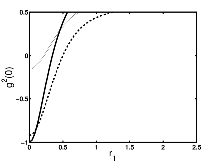
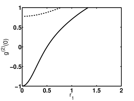
Figure 2: Second-order correlation of the first mode against $r_{1}$. (a) $(n_{1},n_{2},n_{3})=(1,1,1)$, $(r_{2},r_{3})=(r_{1},r_{1})$ solid curve, $(0.1,0.2)$ dashed curve, and $(0.4,0.6)$ dotted curve. (b) $(r_{2},r_{3})=(r_{1},r_{1})$, $(n_{1},n_{2},n_{3})=(1,0,0)$ solid curve and $(0,1,0)$ dashed curve.

$$\begin{array}[]{lr}\langle{\hat{a}_{1}^{\dagger}\hat{a}_{1}}\rangle=n_{1}f_{1}^{(1)2}+(n_{1}+1)f_{2}^{(1)2}+n_{2}g_{1}^{(1)2}+(n_{2}+1)g_{2}^{(1)2}+n_{3}h_{1}^{(1)2}+(n_{3}+1)h_{2}^{(1)2},\\ \\ \langle{\hat{a}_{1}^{\dagger 2}\hat{a}_{1}^{2}}\rangle=n_{1}(n_{1}-1)f_{1}^{(1)4}+(n_{1}+1)(n_{1}+2)f_{2}^{(1)4}+(2n_{1}+1)^{2}f_{1}^{(1)2}f_{2}^{(1)2}\\ \\ +n_{2}(n_{2}-1)g_{1}^{(1)4}+(n_{2}+1)(n_{2}+2)g_{2}^{(1)4}+(2n_{2}+1)^{2}g_{1}^{(1)2}g_{2}^{(1)2}\\ \\ +n_{3}(n_{3}-1)h_{1}^{(1)4}+(n_{3}+1)(n_{3}+2)h_{2}^{(1)4}+(2n_{3}+1)^{2}h_{1}^{(1)2}h_{2}^{(1)2}\\ \\ +(2n_{1}+1)f_{1}^{(1)}f_{2}^{(1)}[2(2n_{2}+1)g_{1}^{(1)}g_{2}^{(1)}+(2n_{3}+1)h_{1}^{(1)}h_{2}^{(1)}]\\ \\ +(2n_{3}+1)h_{1}^{(1)}h_{2}^{(1)}[2(2n_{2}+1)g_{1}^{(1)}g_{2}^{(1)}+(2n_{1}+1)f_{1}^{(1)}f_{2}^{(1)}]\\ \\ +4[n_{1}f_{1}^{(1)2}+(n_{1}+1)f_{2}^{(1)2}][n_{2}g_{1}^{(1)2}+(n_{2}+1)g_{2}^{(1)2}+n_{3}h_{1}^{(1)2}+(n_{3}+1)h_{2}^{(1)2}]\\ \\ +4[n_{2}g_{1}^{(1)2}+(n_{2}+1)g_{2}^{(1)2}][n_{3}h_{1}^{(1)2}+(n_{3}+1)h_{2}^{(1)2}].\end{array}$$ (40)

By means of (24) and (40), the quantity $g_{1}^{(2)}(0)$ is depicted in Figs. 2 for given values of the parameters. In Fig. 2(a) we present the role of the squeezing parameters $r_{j}$ on the behavior of the $g_{1}^{(2)}(0)$. From the solid curve (, i.e. symmetric case), one can observe that the maximum sub-Piossonian statistics occur for relatively small values of $r_{j}$. In this case, the system tends to the Fock state $|1\rangle$, which is a pure nonclassical state. As the values of $r_{1}$ increase, the nonclassicality monotonically decreases and completely vanishes around $r_{1}\simeq 0.3$. Comparison among the curves in Fig. 2(a) shows when the values of $(r_{2},r_{3})$ increase, the amounts of the sub-Poissonian statistics inherited in the first mode decrease. This is connected with the nature of the operator (3), in which the behavior of the single-mode undergoes an amplification process caused by the various down-conversions involved in the system. Furthermore, particular values of the asymmetry can enlarge the range of nonclassicality (compare the solid curve to the dashed one). Now, we draw the attention to the Fig. 2(b), which is given to the symmetric case . From this figure one realizes how can obtain sub-Poissonian statistics from a particular mode as an output from the operator (3). Precisely, this mode should be initially prepared in the nonclassical state. We can analytically prove this fact by substituting $n_{1}=0,n_{2}=n_{3}=n$ into (24) and (40). After minor algebra, we arrive at:

$$\begin{array}[]{lr}\langle\hat{a}_{1}^{\dagger 2}\hat{a}^{2}_{1}\rangle-\langle{\hat{a}^{\dagger}_{1}\hat{a}_{1}}\rangle^{2}=f_{2}^{(1)4}+2n(n-1)g_{1}^{(1)4}+2(n+1)(n+2)g_{2}^{(1)4}\\ +2n(n+1)g_{1}^{(1)2}g_{2}^{(1)2}+[f_{1}^{(1)}f_{2}^{(1)}+2(2n+1)g_{1}^{(1)}g_{2}^{(1)}]^{2}\\ +4f_{2}^{(1)2}[ng_{1}^{(1)2}+(n+1)g_{2}^{(1)2}]\geq 0.\end{array}$$ (44)

The final remark, the comparison between the solid curves in Figs. 2(a) and (b) shows that the nonclassical range of $r_{1}$ in (b) is greater than that in (a). In other words, to enhance the sub-Poissonian statistics in a certain mode, the other modes have to be prepared in states close to the classical ones.

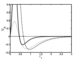
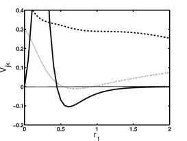
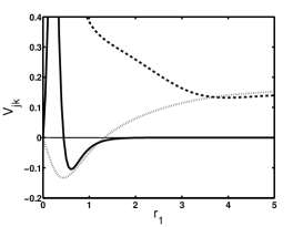
Figure 3: The parameter $V_{jk}$ against $r_{1}$ for the coherent state with $\alpha_{1}=\alpha_{2}=\alpha_{3}=1$, where $(j,k)=(1,2)$ (a), $(1,3)$ (b) and $(2,3)$ (c). Additionally, $(r_{2},r_{3})=(r_{1},r_{1})$ solid curve, $(0.1,0.2)$ dashed curve and $(0.4,0.6)$ dotted curve.

The violation of the classical inequalities has verified the quantum theory. Among these inequalities is the Cauchy-Schwarz inequality lou , which its violation provides information on the intermodal correlations in the system. The first observation of this violation was obtained by Clauser, who used an atomic two-photon cascade system [3] . More recently, strong violations using four-wave mixing have been adopted in [4] ; [5] . In addition, a frequency analysis has been used to infer the violation of this inequality over a limited frequency regime [11] . The Cauchy-Schwarz inequality is $V_{jk}\leq 0$, where $V_{jk}$ has the form:

$$V_{jk}=\frac{\sqrt{\langle\hat{a}^{\dagger 2}_{j}\hat{a}^{2}_{j}\rangle\langle\hat{a}^{\dagger 2}_{k}\hat{a}^{2}_{k}\rangle}}{\langle\hat{a}_{j}^{\dagger}\hat{a}_{j}\hat{a}_{k}^{\dagger}\hat{a}_{k}\rangle}-1.$$ (45)

Occurrence of the negative values in $V_{jk}$ means that the intermodal correlation is larger than the correlation among the photons in the same mode. This indicates a strong deviation from the classical Cauchy-Schwarz inequality. This is related to the quantum mechanical features, which include pseudodistributions instead of the true ones. In this respect, the Glauber-Sudarshan $P$ function possesses strong quantum properties [27] .

Figure 4: The parameter $V_{jk}$ against $r_{1}$ for the Fock-state case with $n_{1}=n_{2}=n_{3}=1$, where $(j,k)=(1,2)$. Additionally, $(r_{2},r_{3})=(r_{1},r_{1})$ solid curve, $(0.1,0.2)$ dashed curve and $(0.4,0.6)$ dotted curve.

We have found that the Cauchy-Schwartz inequality can be violated for both coherent- and number-state cases. The expressions of the different quantities in (45) are too lengthy but straightforward and hence we don’t present them here. We start with the three-mode squeezed coherent states. Information about them is shown in Figs. 3(a), (b) and (c), for given values of the system parameters. The negative values are remarkable in most of the curves, reflecting the deviation from the classical inequality. For the symmetric case the nonclassical correlation is remarkable for $r_{1}\geq 0.4$, which increases gradually till $r_{1}\simeq 0.6$ providing its maximum value, then smoothly reduces and eventually goes to zero, i.e. $V_{jk}\simeq 0$, for large $r_{1}$. For the asymmetric case, the deviation from the classical inequality is obvious, which may be smaller or greater than those in the symmetric one based on the competition among different nonlinearities in the system $r_{j}$. In other words, e.g., the correlation between modes $1$ and $2$ is much stronger than that between the others only when $r_{1}>r_{2},r_{3}$. This can be understood from the structure of the operator (3). Comparing this behavior to that of the two-mode squeezing given in the preceding section one can conclude that a large amount of squeezing does not imply large violation of the inequality carmich . As we mentioned before: the entanglement is a direct consequence of the occurrence of the nonclassical effects. As a result of this, the behavior of the two-mode squeezing and $V_{jk}$ may provide a type of contradiction. Precisely, the bipartite can be entangled (non-entangled) with respect to, say, two-mode squeezing ($V_{jk}$). This supports the fact that these two quantities provide only a sufficient condition for entanglement. Considering both of them we may obtain conditions closer to the necessary and sufficient condition. A study about this controversial issue has been already discussed for the entanglement in a parametric converter suh , where different entanglement criteria leaded to different results.

In Fig. 4 we plot the parameter $V_{jk}$ for the Fock-state case. From this figure the deviation from the classical $V_{jk}$ is quite remarkable. For the symmetric case, maximum deviation occurs in $V_{1,2}$ for $r=0$, monotonically decreases as $r$ evolving and vanishes at $r\simeq 1$. Comparison among different curves in this figure shows that the asymmetry can enlarge the range of $r_{1}$ over which the deviation of the inequality occurs. Similar behavior has been observed for $V_{2,3}$ and $V_{1,3}$ (we have checked this fact). In conclusion, the violation of the classical inequalities provides an explicit evidence of the quantum nature of intermodal correlation between modes. This is not surprising, as the entanglement is a pure quantum mechanical phenomenon that requires a certain degree of nonclassicality either in the initial state or in the process that governs the system.

V Quasiprobability distribution function

Quasiprobability distribution functions, namely, Husimi function ($Q$), Wigner function ($W$), and Glauber $P$ functions, are very important since they can give a global description of the nonclassical effects in the quantum systems. These functions can be measured by various means, e.g. photon counting experiments [34] , using simple experiments similar to that used in the cavity (QED) and ion traps [35] ; [36] , and homodyne tomography [37] . For the system under consideration, we focus the attention here on the single-mode case, say, the first mode for the three-mode squeezed number states (11). We start with the $s-$parameterized characteristic function $C(\zeta,s)$, which is defined as:

$$C(\zeta,s)={\rm Tr}[\hat{\rho}\exp(\zeta\hat{a}^{{\dagger}}_{1}-\zeta^{*}\hat{a}_{1}+\frac{s}{2}|\zeta|)],$$ (46)

where $\hat{\rho}$ is the density matrix of the system under consideration and $s$ is a parameter taking the values $0,1,-1$ corresponding to symmetrically, normally and antinormally ordered characteristic functions, respectively. For three-mode squeezed number states and with the help of the relations (4) one can easily obtain:

$$\begin{array}[]{lr}C(\zeta,s)=\exp[-\frac{1}{2}|\upsilon_{1}|^{2}-\frac{1}{2}|\upsilon_{2}|^{2}-\frac{1}{2}|\upsilon_{3}|^{2}+\frac{s}{2}|\zeta|^{2}]\\ \times{\rm L}_{n_{1}}(|\upsilon_{1}|^{2}){\rm L}_{n_{2}}(|\upsilon_{2}|^{2}){\rm L}_{n_{3}}(|\upsilon_{3}|^{2}),\end{array}$$ (49)

where

$$\upsilon_{1}=\zeta f_{1}^{(1)}-\zeta^{*}f_{2}^{(1)},\quad\upsilon_{2}=\zeta g_{1}^{(1)}-\zeta^{*}g_{2}^{(1)},\quad\upsilon_{3}=\zeta h_{1}^{(1)}-\zeta^{*}h_{2}^{(1)}$$ (50)

and ${\rm L}_{k}^{\gamma}(.)$ is the associated Laguerre polynomial having the form:

$${\rm L}_{k}^{\gamma}(x)=\sum\limits_{l=0}^{k}\frac{(\gamma+k)!(-x)^{l}}{(\gamma+l)!(k-l)!l!}.$$ (51)

The $s$-parameterized quasiprobability distribution functions are defined as

$$W(z,s)=\pi^{-2}\int d^{2}\zeta C(\zeta,s)\exp(z\zeta^{*}-\zeta z^{*}),$$ (52)

where $z=x+iy$ and $s=0,1,-1$ are corresponding to $W,P,Q$ functions, respectively. On substituting (49) into (52) and applying the method of the differentiation under the sign of integration we can obtain the following expression:

$$\begin{array}[]{lr}W(z,s)=\frac{1}{\pi}\sum\limits_{j^{\prime},j,k=0}^{\{n_{1},n_{2},n_{3}\}}\sum\limits_{l_{1},l_{2}=0}^{\{j^{\prime},j+k\}}\left(\begin{array}[]{c}n_{1}\\ j^{\prime}\end{array}\right)\left(\begin{array}[]{c}n_{2}\\ k\end{array}\right)\left(\begin{array}[]{c}n_{3}\\ j\end{array}\right)\left(\begin{array}[]{c}j^{\prime}\\ l_{1}\end{array}\right)\left(\begin{array}[]{c}j+k\\ l_{2}\end{array}\right)\frac{(-1)^{j+j^{\prime}+k}}{j!j^{\prime}!k!}\\ \times(f_{1}^{(1)2}+f_{2}^{(1)2})^{l_{1}}(g_{1}^{(1)2}+g_{2}^{(1)2})^{l_{2}}(f_{1}^{(1)}f_{2}^{(1)})^{j^{\prime}-l_{1}}(g_{1}^{(1)}g_{2}^{(1)})^{j+k-l_{2}}\frac{\partial^{l_{1}+l_{2}}}{\partial b_{1}^{l_{1}+l_{2}}}|_{b_{1}=0}\frac{\partial^{j+j^{\prime}+k-l_{1}-l_{2}}}{\partial b_{2}^{j+j^{\prime}+k-l_{1}-l_{2}}}|_{b_{2}=0}\\ \times\frac{1}{\sqrt{K}}\exp[-\frac{1}{K}(B|z|^{2}+(z^{2}+z^{*2})(\Lambda_{2}+b_{2})],\end{array}$$ (66)

where

$$\begin{array}[]{lr}\Lambda_{1}=f_{1}^{(1)2}+f_{2}^{(1)2}+g_{1}^{(1)2}+g_{2}^{(1)2}+h_{1}^{(1)2}+h_{2}^{(1)2},\\ \\ \Lambda_{2}=f_{1}^{(1)}f_{2}^{(1)}+g_{1}^{(1)}g_{2}^{(1)}+h_{1}^{(1)}h_{2}^{(1)},\\ \\ B=\frac{1}{2}(\Lambda_{1}-s)-b_{1},\quad K=B^{2}-(\Lambda_{2}+b_{2})^{2}.\end{array}$$ (72)

The correlation between the modes in the system can be realized in $W(z,s)$ as cross terms, e.g. in $\Lambda_{2}$. This can give a qualitative information about the entanglement in the system. For the three-mode squeezed vacuum states (, i.e., $n_{1}=n_{2}=n_{3}=0$) the $W$ function (66) can be expressed as:

$$W(x,y,s)=\frac{1}{\pi\sqrt{\vartheta_{+}\vartheta_{-}}}\exp[-\frac{x^{2}}{\vartheta_{+}}-\frac{y^{2}}{\vartheta_{-}}],$$ (73)

where

$$\begin{array}[]{lr}\vartheta_{+}=2\langle(\Delta\hat{X}_{1})^{2}\rangle-\frac{s}{2},\\ \\ =\frac{1}{2}[(f_{1}^{(1)}+f_{2}^{(1)})^{2}+(g_{1}^{(1)}+g_{2}^{(1)})^{2}+(h_{1}^{(1)}+h_{2}^{(1)})^{2}]-\frac{s}{2},\\ \\ \vartheta_{-}=2\langle(\Delta\hat{Y}_{1})^{2}\rangle-\frac{s}{2},\\ \\ =\frac{1}{2}[(f_{1}^{(1)}-f_{2}^{(1)})^{2}+(g_{1}^{(1)}-g_{2}^{(1)})^{2}+(h_{1}^{(1)}-h_{2}^{(1)})^{2}]-\frac{s}{2}.\end{array}$$ (81)

From (73) and (81) it is evident that the quasidistributions are Gaussians, narrowed in the $y$ direction and expanded in the $x$ direction. Nevertheless, this does not mean squeezing is available in this mode. Actually, this behavior represents the thermal squeezed light, which, in this case, is a super-classical light. Precisely, with $s=0$ the $W$ function exhibits stretched contour, whose area is broader than that of the coherent light. In this regard the phase distribution and the photon-number distribution associated with the single-mode case exhibits a single-peak structure for all values of $r_{j}$. This peak is broader than that of the coherent state, which has the same mean-photon number. Actually, this is a quite common property for the multimode squeezed operators single ; two ; abdalla ; hon ; faisal ; barry ; marce . Thus the single-mode vacuum or coherent states, as outputs from the three concurrent amplifiers described by (3) are not nonclassical states. This agrees with the information given in the sections 3 and 4.

Now we consider two cases: $(n_{1},n_{2},n_{3})=(0,0,n_{3})$ and $(n_{1},n_{2},n_{3})=(n_{1},0,0)$. For the first case, we investigate the influence of the nonclassicality in the third mode on the behavior of the first mode. To do so we substitute $n_{1}=n_{2}=0$ in (66) and after minor algebra we arrive at:

$$\begin{array}[]{lr}W(x,y,s)=\frac{(-1)^{n_{3}}}{\pi\sqrt{(\frac{\Lambda_{1}-s}{2})^{2}-\Lambda_{2}^{2}}}(\frac{\eta_{-}}{\vartheta_{+}})^{n_{3}}\exp[-\frac{x^{2}}{\vartheta_{-}}-\frac{y^{2}}{\vartheta_{+}}]\\ \\ \times\sum\limits_{m=0}^{n_{3}}\left(\frac{\vartheta_{+}\eta_{+}}{\vartheta_{-}\eta_{-}}\right)^{m}{\rm L}_{m}^{-\frac{1}{2}}[(\frac{\eta_{+}+\vartheta_{-}}{\eta_{+}\vartheta_{-}})x^{2}]{\rm L}_{n_{3}-m}^{-\frac{1}{2}}[(\frac{\eta_{-}+\vartheta_{+}}{\eta_{-}\vartheta_{+}})y^{2}],\end{array}$$ (85)

where

$$\eta_{\pm}=(h_{1}^{(1)}\pm h_{2}^{(1)})^{2}-\vartheta_{\mp}.$$ (86)

One can easily check when $r_{1}=r_{2}=r_{3}=0$ the $W$ function (85) reduces to that of the vacuum state. The form (85) includes Laguerre polynomial, which is well known in the literature by providing nonclassical effects in the phase space. This indicates that the nonclasssical effects can be transferred from one mode to another under the action of the operator (3). Of course the amount of the transferred data depends on the values of the squeezing parameters $r_{j}$.

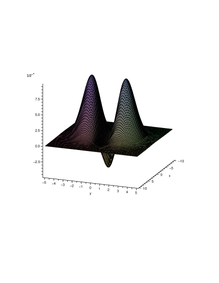
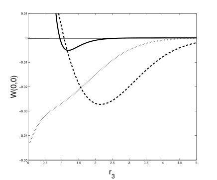
Figure 5: The Wigner function of the first mode (a) and the evolution of the phase space origin of the Wigner function (b). In (a) we use $(r_{1},r_{2},r_{3},n_{1},n_{2},n_{3})=(1.1,1.1,1.1,0,0,1)$. In (b) we use $(r_{1},r_{2},n_{1},n_{2},n_{3})=(r_{3},r_{3},0,0,1)$ solid curve, $(0.6,0.8,0,0,1)$ dashed curve, and $(0.6,0.8,1,0,0)$ dotted curve.

The second case $(n_{1},0,0)$ has the same expression (85) with the following transformations:

$$n_{3}\rightarrow n_{1},\quad\eta_{\pm}=(f_{1}^{(1)}\pm f_{2}^{(1)})^{2}-\vartheta_{\mp}.$$ (87)

Now we prove that this $W$ function tends to that of the number state when $r_{1}=r_{2}=r_{3}=0$. In this case, the transformations (87) tend to:

$$\eta_{\pm}=\frac{1+s}{2},\quad\vartheta_{\pm}=\frac{1-s}{2}.$$ (88)

Substituting these variables in the expression (85) (with $n_{3}\rightarrow n_{1}$) we obtain:

$$\begin{array}[]{lr}W(x,y,s)=\frac{2(-1)^{n_{1}}}{\pi}\frac{(1+s)^{n_{1}}}{(1-s)^{n_{1}+1}}\exp[-\frac{2(x^{2}+y^{2})}{1-s}]\sum\limits_{m=0}^{n_{1}}{\rm L}_{m}^{-\frac{1}{2}}[\frac{4x^{2}}{1-s^{2}}]{\rm L}_{n_{1}-m}^{-\frac{1}{2}}[\frac{4y^{2}}{1-s^{2}}]\\ \\ =\frac{2(-1)^{n_{1}}}{\pi}\frac{(1+s)^{n_{1}}}{(1-s)^{n_{1}+1}}\exp[-\frac{2(x^{2}+y^{2})}{1-s}]{\rm L}_{n_{1}}[\frac{4(x^{2}+y^{2})}{1-s^{2}}],\end{array}$$ (92)

In (92) the transition from the first line to the second one has been done using the identity:

$$\sum\limits_{n=0}^{m}{\rm L}_{n}^{\tau_{1}}(x){\rm L}_{m-n}^{\tau_{2}}(y)={\rm L}_{m}^{\tau_{1}+\tau_{2}+1}(x+y).$$ (93)

The expression (92) is the $s$-quasprobability distribution for the number state, e.g. wolfgang .

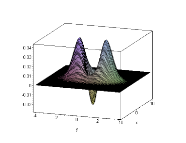
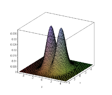
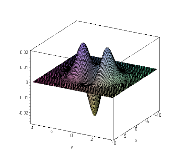
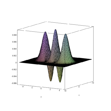
Figure 6: The Wigner function of the first mode when $(r_{1},r_{2},r_{3},n_{1},n_{2},n_{3})=(0.6,0.8,0.9,1,0,0)$ (a), $(0.6,0.8,0.9,0,0,1)$ (b), $(0.6,0.8,2,0,0,1)$ (c) and $(0.4,0.8,2,0,0,2)$ (d).

We conclude this part by writing down the form of the $W$ function at the phase space origin, which is a sensitive point for the occurrence of the nonclassical effects. Moreover, it can simply give visualization about the behavior of the system. Additionally, this point can be measured by the photon counting method [34] . From (85) we have:

$$W(0,0,s)=\frac{(-1)^{n_{3}}}{\pi\sqrt{\vartheta_{+}\vartheta_{-}}}(\frac{\eta_{-}}{\vartheta_{+}}+\frac{\eta_{+}}{\vartheta_{-}})^{n_{3}}.$$ (94)

It is obvious that the Winger function exhibits negative values at the phase space origin only when $n_{3}$ is an odd number.

In Figs. 5 and 6 we plot the $W$ functions for the given values of the system parameters. We start the discussion with the symmetric case. In Fig. 5(a) we use $(n_{1},n_{2},n_{3})=(0,0,1)$ meaning that the mode under consideration is in the vacuum state. Thus for $r_{j}=0$ the $W$ function exhibits the single-peak-Gaussian structure with a center at the phase space origin. When $r_{j}\neq 0$ this behavior is completely changed, where one can observe a lot of the nonclassical features, e.g. negative values, multipeak structure and stretching contour (see Fig. 5(a)). This indicates that the nonclassical effects can be transferred from one mode to the other under the action of the operator (3). In Fig. 5(b) we plot the ”evolution” of the $W$ function given by (94) against the parameter $r\quad(r_{3})$ for the symmetric (asymmetric) case. The aim of this figure is to estimate the exact value of the nonlinearity $r\quad(r_{3})$ for which the nonclassical effects maximally occur and/or transfer from certain mode to the other. For the symmetric case, this occurs at $r=1.2$, while the nonclassicality is completely washed out at $r=3$. Now, we draw the attention to the asymmetric case which is plotted in Figs. 6. Fig. 6(a) gives information on the case $(n_{1},n_{2},n_{3})=(1,0,0)$. The $W$ function of the Fock state $|1\rangle$ is well known in the literatures by having inverted peak in phase space with maximum negative values. This is related to that this state provides maximum sub-Poissonian statistics. Under the action of the operator (3) these negative values are reduced and the two-peak structure is started to be constructed. This indicates that the system is able to generate particular types of the Schrödinger-cat states by controlling the system parameters. This is really obvious in Figs. 6(b)–(d), which are given to the cases $n_{1}=n_{2}=0,n_{3}=1,2$. For instance, from Fig. 6(b) the $W$ function provides a two-peak structure. Nevertheless, by increasing the values of the parameter $r_{3}$, the $W$ function exhibits the two Gaussian peaks and inverted negative peak in-between indicating the occurrence of the interference in phase space (see Fig. 6(c)). This shape is similar to that of the odd-coherent state. Additionally, the Fig. 6(d), in which $n_{3}=2$, provides the well-known shape of the $W$ function of the even coherent state. Generally, the even and the odd Schrödinger-cat states have nearly identical classical components (, i.e. the positive peaks) and only differ in the sign of their quantum interferences. These are interesting results, which show that by controlling the nonlinearity of the system and preparing a certain mode in the Fock state $|1\rangle$ or $|2\rangle$ one can generate cat states. It is worth mentioning that the Fock state $|n\rangle$ can be prepared with very high efficiency according to the recent experiments [48] . Similar results have been obtained from the codirectional three-mode Kerr nonlinear coupler faisalcoupler . Furthermore, quite recently the construction of the cat state trapped in the cavity in which several photons survive long enough to be repeatedly measured is given in haroche . In this technique, the atoms crossing the cavity one by one are used to obtain information about the field. We proceed, we have noted that the $W$ function of the cases $n_{2}=n_{3}=0,n_{1}=1,2$ can provide quite similar behaviors as those of Figs. 6(c) and (d) for the same values of $r_{j}$. Now, we draw the attention to the dashed and dotted curves in the Fig. 5(b). These curves provide information on the evolution of the $W(0,0)$ against $r_{3}$ for the case of Fig. 6(a) and (c), respectively. From the dotted curve, i.e. the mode under consideration is in the Fock state, the $W(0,0)$ exhibits the maximum negativity at $r_{3}=0$, which monotonically decreases and completely vanishes at $r_{3}=4$. This shows for how long the nonclassicality inherited in the first mode survives based on the intensity of the third amplifier. On the other hand, form the dashed curve, i.e. the mode under consideration is in the vacuum state, the $W(0,0)$ exhibits negative values for $r_{3}\geq 1$, increases rapidly to show maximum around $r_{3}=2$, reduces gradually and vanishes for $r_{3}\geq 5$. This range of negativity is greater than that of the dotted curve. This is in a good agrement with the behavior of the second-order correlation function. Finally, comparison among the curves in Fig. 5(b) confirms the fact: for certain values of the system parameters, the asymmetric case can provide nonclassical effects greater than those of the symmetric one.

VI Conclusion

In this paper we have studied the three-mode squeezed operator, which can be implemented from the triply coincident nonlinearities in periodically poled $KTiOPO_{4}$. The action of this operator on the three-mode coherent and number states is demonstrated. We have studied quadrature squeezing, second-order correlation function, Cauchy-Schwartz inequality and quasiprobability distribution function. The obtained results can be summarized as follows. Generally, the single-mode vacuum or coherent states, as outputs from the three concurrent amplifiers are not nonclassical states. The system can exhibit two-mode and three-mode squeezing. The amount of the two-mode squeezing generated by the asymmetric case is much greater than that of the symmetric case. Three-mode squeezed coherent (number) states cannot (can) exhibit sub-Poissonian statistics. To obtain maximum sub-Poissonian statistics from a particular mode, under the action of the operator (3), it must be prepared in the nonclassical state and the other modes in states close to the classical ones. We have found that the Cauchy-Schwartz inequality can be violated for both coherent states and number states. The origin in the violation is in the strong quantum correlation among different modes. For the Fock-state case, the asymmetry in the system enhances the range of nonlinearities for which $V_{jk}$ is nonclassical compared to that of the symmetric one. In the framework of the quasiprobability distribution we have shown that the nonclassical effects can be transferred from one mode to another under the action of the operator (3). The amount of transferred nonclassicality is sensitive to the values of the squeezing parameters. Interestingly, the system can generate particular types of the Schrödinger-cat states for certain values of the system parameters. Generally, we have found that the nonclassical effects generated by the operator (3) are greater than those obtained from the operator TMS faisal . Finally, the asymmetry in the three concurrent nonlinearities process is important for obtaining significant nonclassical effects.

References

References

- (1) Hillery M 2000 Phys. Rev. A 61 022309.
- (2) Ekert A K 1991 Phys. Rev. Lett. 67 661; Bennett C H, Brassard G and Mermin N D 1992 Phys. Rev. Lett. 68 557.
- (3) Loock P V and Braunstein S L 2000 Phys. Rev. Lett. 84 3482.
- (4) Loock P V and Braunstein S L 2001 Phys. Rev. Lett. 87 247901.
- (5) Jing J, Zhang J, Yang Y, Zhao F, Xie C and Peng K 2003 Phys. Rev. Lett. 90 167903.
- (6) Guo J, Zou H, Zhai Z, Zhang J and Jiangrui 2005 Phys. Rev. A 71 034305.
- (7) Olsen M K, Bradley A S and Reid M D 2006 J Phy B: At. Mol. Opt. Phys. 39 2515; Bradley A S, Olsen M K, Pfister O and Pooser R C 2005 Phys. Rev. A 72 053805.
- (8) Pfister O, Feng S, Jennings G, Pooser R C and Xie D 2004 Phys. Rev. A 70 020302(R); Pooser R C and Pfister O 2005 Opt. Lett. 30 2635.
- (9) Tan H-T; Li G-X and Zhu S-Y 2007 Phys. Rev. A 75 063815.
- (10) Loock P V and Furusawa A 2000 Phys. Rev. A. 67 052315.
- (11) Yuen H P 1976 Phys. Rev. A 13 2226; Caves C M 1981 Phys. Rev. D. 23 1693.
- (12) Barnett S M and Knight P L 1985 J Opt. Soc. Am. B 2 467; Barnett S M and Knight P L 1987 J. Mod. Opt. 34 841; Gilles L and Knight P L 1992 J. Mod. Opt. 39 1411.
- (13) Abdalla M S 1992 J. Mod. Opt. 39 771; ibid. 39 1067; 1993 ibid. 40 441; ibid. 40 1369; Abdalla M S and Obada A-S F 2000 Int. J. Mod. Phys. 14 1105.
- (14) Abdalla M S, El-Orany F A A and Peřina J 2001 Eur. Phys. J. D. 13, 423.
- (15) Shaterzadeh-Yazdi Z, Turner P S and Sanders B C 2008 J. Phys. A: Math. Theor. 41 055309.
- (16) Hu L-Y and Fan H-Y 2009 EPL 85 60001.
- (17) Marchiolli M A and Galetti D 2008 Phys. Scr. 78 045007.
- (18) Loock P V and Braunstein S L 2003 Quantum Information with Continuous Variables, eds. Braunstein S L and Pati A K (Kluwer Academic, Dordrecht), P. 138.
- (19) Braunstein S L and Kimble H J 1998 Phys. Rev. Lett. 80 869; Milburn G J and Braunstein S L 1999 Phys. Rev. A 60 937; Ralph T C 2000 Phys. Rev. A 61 010303(R).
- (20) Lee S-Y, Qamar S, Lee H-W and Zubairy M S 2008 J. Phys. B: At. Mol. Opt. Phys. 41 145504.
- (21) Braunstein S L and Loock P V 2005 Rev. Mod. Phy. 77 513.
- (22) Dagenis M and Mandel L 1978 Phys. Rev. A 18 2217.
- (23) Carmichael H J and Walls D F 1976 J. Phys. 9B L43; Kimble H J and Mandel L 1976 Phys. Rev. A 13 2123.
- (24) Loudon R 1980 Rep. Prog. Phys. 43 913; Reid M D and Walls D F 1986 Phys. Rev. A 34 1260.
- (25) Clauser J F 1974 Phys. Rev. D 9 853.
- (26) Kolchin P, Du S, Belthangady C, Yin G Y and Harris S E 2006 Phys. Rev. Lett. 97 113602.
- (27) Thompson J K, Simon J, Loh H and Vuletic V 2006 Science 313 74.
- (28) Li Y-q, Edwards P J, Huang X and Wang Y 2000 J. Opt. B 2 292; Marino A M, Boyer V and Lett P D quant-ph/0802.3183.
- (29) Agarwal G S 1988 J. Opt. Soc. Am. B 5 1940.
- (30) Carmichael H J, Castro-Beltran H M, Foster G T and Orozco L A 2000 Phys. Rev. Lett. 85 1855.
- (31) Banaszek K and W dkiewicz k 1996 Phys. Rev. Lett. 76 4344; Wallentowitz S and Vogel W 1996 Phys. Rev. A 53 4528.
- (32) Lutterbach L G and Davidovich L 1997 Phys. Rev. Lett. 78 2547.
- (33) Nogues G, Rauschenbeutel A, Osnaghi S, Bertet P, Brune M, Raimond J M, Haroche S, Lutterbach L G and Davidovich L 2000 Phys. Rev. A 62 054101.
- (34) Beck M, Smithey D T and Raymer M G 1993 Phys. Rev. A 48 890; Smithey D T, Beck M, Cooper J and Raymer M G 1993 Phys. Rev. A 48 3159; Beck M, Smithey D T, Cooper J and Raymer M G 1993 Opt. Lett. 18 1259; Smithey D T, Beck M, Cooper J, Raymer M G and Faridani M B A 1993 Phys. Scr. T 48 35.
- (35) Schleich W P 2001 ”Quantum optics in phase space” (Wiley-VCH Verlag, Berlin)
- (36) El-Orany F A A, Abdalla M S and Peřina J 2005 Eur. Phys. J. D 33 453.
- (37) Leibfried D, Meekhof D M, King B E, Monroe C, Itano W M and Wineland D J 1996 Phys. Rev. Lett. 77 4281; Meekhof D M, Monroe C, King B E, Itano W M and Wineland D J 1996 Phys. Rev. Lett. 76 1796; Monroe C, Meekhof D M, King B E and Wineland D J 1996 Science 272 1131.
- (38) Deleglise S, Dotsenko I, Sayrin C, Bernu J, Brune M, Raimond J-M and Haroche S 2008 nature 455 510.