Linear atomic quantum coupler

Abstract

In this paper, we develop the notion of the linear atomic quantum coupler. This device consists of two modes propagating into two waveguides, each of them includes a localized and/or a trapped atom. These waveguides are placed close enough to allow exchanging energy between them via evanescent waves. Each mode interacts with the atom in the same waveguide in the standard way, i.e. as the Jaynes-Cummings model (JCM), and with the atom-mode in the second waveguide via evanescent wave. We present the Hamiltonian for the system and deduce the exact form for the wavefunction. We investigate the atomic inversions and the second-order correlation function. In contrast to the conventional linear coupler, the atomic quantum coupler is able to generate nonclassical effects. The atomic inversions can exhibit long revival-collapse phenomenon as well as subsidiary revivals based on the competition among the switching mechanisms in the system. Finally, under certain conditions, the system can yield the results of the two-mode JCM.

I Introduction

Quantum directional coupler is a device composed of two (or more) waveguides placed close enough to allow exchanging energy between them via evanescent waves jen1 . The rate of flow of the exchanged energy can be controlled by the device design and the intensity of the input flux as well. The outgoing fields from the coupler can be examined in the standard ways to observe the nonclassical effects. Quite recently, this device has attracted much attention in the framework of the optics communication and quantum computing networks qcoup , which require data transmission and ultra-high-speed data processing EKer1 . Furthermore, the directional coupler has been experimentally implemented, e.g. in planar structures exp1 , dual optical fibres exp2 and certain organic polymers exp3 . For more details related to the quantum properties of the fields in the directional couplers the reader can consult the review paper qu20 and the references therein.

The interaction between the radiation field and the matter (, i.e. atom), namely, Jaynes-Cummings model (JCM) jay1 , is an important topic in the quantum optics and quantum information theories kni . The simplest form of the JCM is the two-level atom interacting with the single-mode of the radiation field. The JCM is a rich source for the nonclassical effects, e.g. the revival-collapse phenomenon (RCP) eber , sub-Poissonian statistics and squeezing fa . Furthermore, the JCM has been experimentally implemented by various means, e.g. one-atom mazer remp , the NMR refocusing meu , a Rydberg atom in a superconducting cavity sup , the trapped ion vogele and the micromaser micr . Various extensions to the JCM have been reported including the two two-level atoms interacting with the radiation field(s) tess ; faisalob .

The trapped atoms or molecules are promising systems for quantum information processing and communications Nielsen . They can serve as convenient and robust quantum memories for photons, providing thereby an interface between static and flying qubits Lukin . The subject of coupling cold atoms to the radiation field sustained by an optical waveguide has already appeared in various contexts. For example, hollow optical glass fibers were used to guide atoms over long distances Noh , especially, employing red detuned light field filling out the hollow core Letokhov ; Renn . Substrate based atom waveguide can also be realized by using guided two-color evanescent light fields Barnett . Moreover, the coupling of atomic dipoles to the evanescent field of tapered optical fibers has been demonstrated in Vetsch ; Nayak . In this respect the optical nanofibers can manipulate and probe single-atom fluorescence. Moreover, it has been suggested that using a two-color evanescent light field around a subwavelength-diameter fiber traps and guides atoms. The optical fiber carries a red-detuned light and a blue-detuned light, with both modes far from resonance. When both input light fields are circularly polarized, a set of trapping minima of the total potential in the transverse plane appears as a ring around the fiber. This design allows confinement of atoms to a cylindrical shell around the fiber Kien . Additionally, it has been shown that sub-wavelength diameter optical fibers can be used to detect, spectroscopically investigate, and mechanically manipulate extremely small samples of cold atoms. In particular, on resonance, as little as two atoms on average, coupled to the evanescent field surrounding the fiber, already absorbed 20 of the total power transmitted through the fiber. By optically trapping one or more atoms around such fibers Dowling , it should become possible to deterministically couple the atoms to the guided fiber mode and to even mediate a coupling between two simultaneously trapped atoms Fam . This leads to a number of applications, e.g., in the context of quantum information processing, high precision measurements, single-photon generation in optical fiber or EIT-based parametric four-wave mixing horak using a few atoms around optical nanofibers. Inspired by these facts we develop here the notion of the atomic quantum coupler (AQC), for which the interaction mechanisms inside the waveguides and between the waveguides depend on both the atomic and bosonic systems. These mechanisms are more complicated than those in the JCM, as we shall show shortly. For the AQC we show that the atomic inversions can exhibit long revival-collapse phenomenon as well as subsidiary-revival patterns based on the switching mechanisms in the system. Furthermore, under certain conditions, the system can give the results of the two-mode JCM. Also, the system is able to generate nonclassical effects. It is worth mentioning that the inclusion of one atom in one of the ports of the non-linear coupler has been considered in abdalla . Nevertheless, the solution of the equations of motion there is obtained by the rotation of axes, which does not give complete information on the system.

We restrict the study in this paper to the development of the Hamiltonian model, its dynamical wavefunction and how does it work. These issues are discussed in section II. Additionally, in section III, we study two quantities, namely, the atomic inversions and the second-order correlation functions.

II Model formalism and its wavefunction

In this section we describe the linear directional atomic quantum coupler (AQC) and derive its wavefunction. Also we discuss some basic differences between this device and the conventional directional coupler qu20 . Thus it is reasonable to shed some light on the linear directional coupler, which is described by the following Hamiltonian qu20 :

$$\frac{\hat{H}}{\hbar}=\sum_{j=1}^{2}\omega_{j}\hat{a}_{j}^{\dagger}\hat{a}_{j}+\lambda(\hat{a}_{1}\hat{a}_{2}^{\dagger}+\hat{a}_{1}^{\dagger}\hat{a}_{2}),$$ (1)

where $\hat{a}_{1}\quad(\hat{a}_{1}^{\dagger})$ and $\hat{a}_{2}\quad(\hat{a}_{2}^{\dagger}$) are the annihilation (creation) operators of the first and the second modes in the first and the second waveguides with the frequencies $\omega_{1}$ and $\omega_{2}$; $\lambda$ is the coupling constant between the waveguides. Basically this device operates as a quantum switcher since it can switch the nonclassical effects as well as the intensities of the modes propagating inside one of the waveguides to the other jans . In other words, it can not generate nonclassical effects by itself. For some reason that will be clear shortly, we calculate the mean-photon numbers for the Hamiltonian (1) when the two modes are in the states $|\alpha,0\rangle$. Thus we arrive at:

$$\langle\hat{a}_{1}^{\dagger}(T)\hat{a}_{1}(T)\rangle=|\alpha|^{2}\cos^{2}(T),\quad\langle\hat{a}_{2}^{\dagger}(T)\hat{a}_{2}(T)\rangle=|\alpha|^{2}\sin^{2}(T),$$ (2)

where $T=\lambda t$. These equations indicate strong switching mechanism in the linear coupler, where the intensity $|\alpha|^{2}$ in the first waveguide has been completely switched to the other one. Moreover, the mean-photon numbers can not exhibit the RCP.

Now we are in a position to develop the AQC, which is the main object of the paper. The atomic coupler consists of two waveguides, each of which includes a localized and/or a trapped atom. The wavegudies are placed close enough to each other to allow interchanging energy between them. The two atoms (in the different waveguides) are located very adjacent to each other. In each waveguide one mode propagates along and interacts with the atom inside in a standard way as the JCM. The atom-mode in each waveguide interacts with the other one via the evanescent wave. The fields exited from the coupler can be examined as single or compound modes by means of homodyne detection to observe the squeezing of vacuum fluctuations, or by means of a set of photodetectors to measure photon antibunching and sub-Poissonian photon statistics in the standard ways. The scheme for the AQC is depicted in Fig. 1. From this figure and in the framework of the rotating wave approximation (RWA) the Hamiltonian describing the AQC can be expressed as:

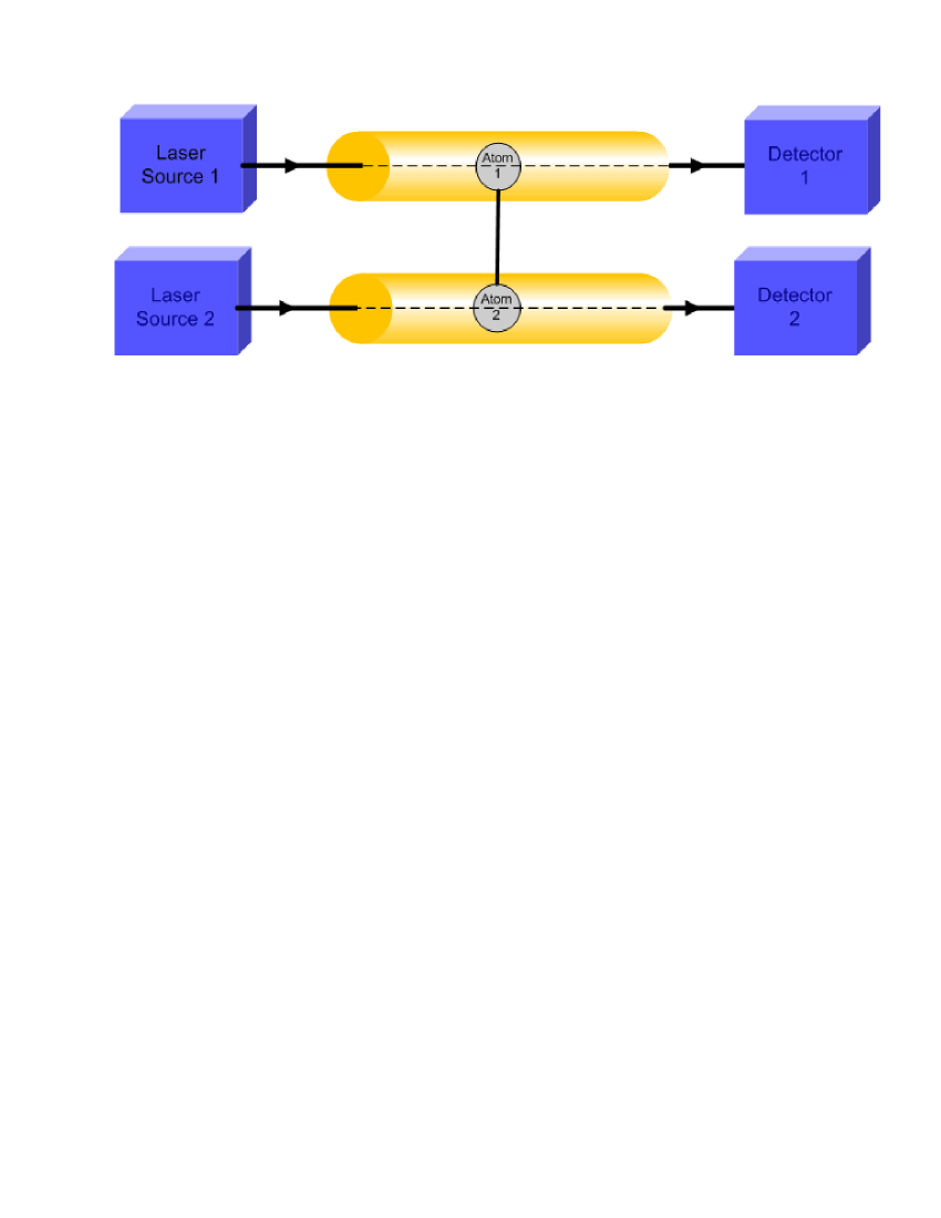
Figure 1: Scheme of realization of the Hamiltonian (3). It is composed from two optical waveguides (yellow color). The circles in these waveguides denote the localized and/or trapped atoms. Mode 1 (2) pumped by, e.g., laser sources propagates along the first (second) waveguide and interacts with the first (second) atom via the coupling constant $\lambda_{1}\quad(\lambda_{2})$. The interaction between the first and the second waveguide occurs via the evanescent wave with the coupling constant $\lambda_{3}$. The outgoing fields from the coupler can be measured in the standard ways, e.g., using photon detectors.

$$\begin{array}[]{lr}\frac{\hat{H}}{\hbar}=\hat{H}_{0}+\hat{H}_{I},\\ \\ \hat{H}_{0}=\sum\limits_{j=0}^{2}\omega_{j}\hat{a}_{j}^{\dagger}\hat{a}_{j}+\frac{\omega_{a}}{2}(\hat{\sigma}_{z}^{(1)}+\hat{\sigma}_{z}^{(2)}),\quad\hat{H}_{I}=\sum\limits_{j=1}^{2}\lambda_{j}(\hat{a}_{j}\hat{\sigma}_{+}^{(j)}+\hat{a}_{j}^{\dagger}\hat{\sigma}_{-}^{(j)})+\lambda_{3}(\hat{a}_{1}\hat{a}_{2}^{\dagger}\hat{\sigma}_{+}^{(1)}\hat{\sigma}_{-}^{(2)}+\hat{a}_{1}^{\dagger}\hat{a}_{2}\hat{\sigma}_{-}^{(1)}\hat{\sigma}_{+}^{(2)}),\end{array}$$ (6)

where $\hat{H}_{0}$ and $\hat{H}_{I}$ are the free and the interaction parts of the Hamiltonian, $\hat{\sigma}_{\pm}^{(j)}$ and $\hat{\sigma}_{z}^{(j)}$ are the Pauli spin operators of the $j$th atom ($j=1,2$); $\hat{a}_{j}\quad(\hat{a}_{j}^{\dagger})$ is the annihilation (creation) operator of the $j$th-mode with the frequency $\omega_{j}$ and $\omega_{a}$ is the atomic transition frequency (we consider that the frequencies of the two atoms are equal) and $\lambda_{1}\quad(\lambda_{2})$ is the atom-field coupling constant in the first (second) waveguide in the framework of the JCM. The derivation of the JCM Hamiltonian is well known, e.g. lo . The interaction between the modes in the two waveguides occurs through the evanescent wave with the coupling constant $\lambda_{3}$. This term is the only one, which is conservative and can execute switching between the two waveguides. Thus it plays an essential role in the behavior of the AQC. We should stress that the switching mechanism occurs through the two JCMs (in the two waveguides) and can be obtained by applying the RWA in each individual waveguide. In other words, the quantity $\lambda_{3}(\hat{a}_{1}\hat{\sigma}_{-}^{(1)}\hat{a}_{2}^{\dagger}\hat{\sigma}_{+}^{(2)}+\hat{a}_{1}^{\dagger}\hat{\sigma}_{+}^{(1)}\hat{a}_{2}\hat{\sigma}_{-}^{(2)})$ is nonconservative and hence it is cancelled out. Finally, the treatment of the switching mechanism in (6) is related to the notion of coupler, however, the existence of atoms in the waveguides has been taken into account. In (6) the treatment is considered only at the moment when the two fields interacting with atoms in the waveguides. Also when we treat the atoms (fields) classically the Hamiltonian (6) tends to that of the linear directional coupler (two-atom interaction).

The interaction of two two-level atoms with the two modes has been considered in the optical cavity earlier faisalob ; eberlyy ; Federico , however, in the sense different from that presented above. For instance, as a sum of two separate Jaynes-Cummings Hamiltonians to investigate the entanglement eberlyy as well as the entanglement transfer from a bipartite continuous-variable (CV) system to a pair of localized qubits Federico . Also, the quantum properties of the system of two two-level atoms interacting with the two nondegenerate cavity modes when the atoms and the field are initially in the atomic superposition states and the pair-coherent state has been investigated in faisalob .

Next, we evaluate the wave function for the Hamiltonian (6). We assume that the two modes and atoms are initially prepared in the coherent states $|\alpha,\beta\rangle$ and in the excited atomic states $|e_{1},e_{2}\rangle$, respectively. For resonance case $2\omega_{a}=\omega_{1}+\omega_{2}$ one can easily prove that $[\hat{H}_{0},\hat{H}_{I}]=0$. Under these conditions, the dynamical wave function describing the system can be expressed as:

$$\begin{array}[]{lr}\mid\Psi(t)\rangle=\sum\limits_{n,m=0}^{\infty}C_{n,m}\left[X_{1}(t,n,m)\mid e_{1},e_{2},n,m\rangle+X_{2}(t,n,m)\mid e_{1},g_{2},n,m+1\rangle\right.\\ \\ +\left.X_{3}(t,n,m)\mid g_{1},e_{2},n+1,m\rangle+X_{4}(t,n,m)\mid g_{1},g_{2,}n+1,m+1\rangle\right],\\ \\ C_{n,m}=\exp(-\frac{1}{2}|\alpha|^{2}-\frac{1}{2}|\beta|^{2})\frac{\alpha^{n}\beta^{m}}{\sqrt{n!m!}},\end{array}$$ (12)

where $|g\rangle$ stands for atomic ground state. From the Schrödinger equation we obtain the following system of differential equations:

$$\begin{array}[]{lr}i\dot{X}_{1}(t,n,m)=\lambda_{2}\sqrt{m+1}X_{2}(t,n,m)+\lambda_{1}\sqrt{n+1}X_{3}(t,n,m),\\ i\dot{X}_{2}(t,n,m)=\lambda_{2}\sqrt{m+1}X_{1}(t,n,m)+\lambda_{3}\sqrt{(n+1)(m+1)}X_{3}(t,n,m)+\lambda_{1}\sqrt{n+1}X_{4}(t,n,m),\\ i\dot{X}_{3}(t,n,m)=\lambda_{1}\sqrt{n+1}X_{1}(t,n,m)+\lambda_{3}\sqrt{(n+1)(m+1)}X_{2}(t,n,m)+\lambda_{2}\sqrt{m+1}X_{4}(t,n,m),\\ i\dot{X}_{4}(t,n,m)=\lambda_{1}\sqrt{n+1}X_{2}(t,n,m)+\lambda_{2}\sqrt{m+1}X_{3}(t,n,m),\end{array}$$ (17)

where the superscript ”.” means differentiation w.r.t. time. In the following, we give only the details related to the solution of the coefficient $X_{1}(t,n,m)$, where the others can be similarly treated. Differentiating the first and last equations in (17) and re-substitute by the others we obtain:

$$\begin{array}[]{lr}(\hat{D}^{2}+A_{n,m})X_{1}(t,n,m)=-(i\lambda_{3}c_{2}D+c_{1})X_{4}(t,n,m),\\ (\hat{D}^{2}+A_{n,m})X_{4}(t,n,m)=-(i\lambda_{3}c_{2}D+c_{1})X_{1}(t,n,m),\\ \hat{D}=\frac{d}{dt},A_{n,m}=\lambda_{1}^{2}(n+1)+\lambda_{2}^{2}(m+1),c_{1}=2\lambda_{1}\lambda_{2}\sqrt{(n+1)(m+1)},c_{2}=\lambda_{3}\sqrt{(n+1)(m+1)}.\end{array}$$ (21)

From (21) one can easily obtain:

$$(\hat{D}^{2}+A_{n,m})^{2}X_{1}(t,n,m)=(i\lambda_{3}c_{2}D+c_{1})^{2}X_{1}(t,n,m).$$ (22)

This equation can be easily solved. By means of the initial conditions stated above the exact forms of the coefficients $X_{j}$ can be expressed as:

$$\begin{array}[]{lr}X_{1}(t,n,m)=\frac{1}{2}\exp(i\frac{t}{2}c_{2})\left[\cos(t\Omega_{-})-i\frac{c_{2}}{2\Omega_{-}}\sin(t\Omega_{-})\right]+\frac{1}{2}\exp(-i\frac{t}{2}c_{2})\left[\cos(t\Omega_{+})+i\frac{c_{2}}{2\Omega_{+}}\sin(t\Omega_{+})\right],\\ \\ X_{2}(t,n,m)=\frac{-i\sqrt{m+1}}{2c_{2}^{2}[A_{n,m}-4\frac{\lambda_{1}^{2}\lambda_{2}^{2}}{\lambda_{3}^{2}}]}\Bigl{\{}\exp(i\frac{t}{2}c_{2})\left[(c_{2}^{2}-2c_{1})\lambda_{2}^{3}(m+1)+(2A_{n,m}-c_{1})\left(\lambda_{2}c_{1}-\frac{\lambda_{1}\lambda_{3}}{2}(n+1)c_{2}\right)\right]\\ \\ \times\frac{\sin(t\Omega_{-})}{\Omega_{-}}+\exp(-i\frac{t}{2}c_{2})\left[(c_{2}^{2}+2c_{1})\lambda_{2}^{3}(m+1)-(2A_{n,m}+c_{1})\left(\lambda_{2}c_{1}-\frac{\lambda_{1}\lambda_{3}}{2}(n+1)c_{2}\right)\right]\frac{\sin(t\Omega_{+})}{\Omega_{+}}\Bigr{\}},\\ \\ X_{3}(t,n,m)=\frac{-i\sqrt{n+1}}{2c_{2}^{2}[A_{n,m}-4\frac{\lambda_{1}^{2}\lambda_{2}^{2}}{\lambda_{3}^{2}}]}\Bigl{\{}\exp(i\frac{t}{2}c_{2})\left[(c_{2}^{2}-2c_{1})\lambda_{1}^{3}(n+1)+(2A_{n,m}-c_{1})\left(\lambda_{1}c_{1}-\frac{\lambda_{2}\lambda_{3}}{2}(m+1)c_{2}\right)\right]\\ \\ \times\frac{\sin(t\Omega_{-})}{\Omega_{-}}+\exp(-i\frac{t}{2}c_{2})\left[(c_{2}^{2}+2c_{1})\lambda_{1}^{3}(n+1)-(2A_{n,m}+c_{1})\left(\lambda_{1}c_{1}-\frac{\lambda_{2}\lambda_{3}}{2}(m+1)c_{2}\right)\right]\frac{\sin(t\Omega_{+})}{\Omega_{+}}\Bigr{\}},\\ \\ X_{4}(t,n,m)=\frac{1}{2}\exp(i\frac{t}{2}c_{2})\left[-\cos(t\Omega_{-})+i\frac{c_{2}}{2\Omega_{-}}\sin(t\Omega_{-})\right]+\frac{1}{2}\exp(-i\frac{t}{2}c_{2})\left[\cos(t\Omega_{+})+i\frac{c_{2}}{2\Omega_{+}}\sin(t\Omega_{+})\right],\end{array}$$ (34)

where

$$\Omega_{\pm}=\frac{1}{2}\sqrt{\lambda_{3}^{2}(n+1)(m+1)+4(\lambda_{1}\sqrt{n+1}\pm\lambda_{2}\sqrt{m+1})^{2}}.$$ (35)

It is obvious that the Rabi oscillation in the AQC is more complicated than that of the JCM. From the solution (34) different limits can be checked. For instance, when $(\lambda_{2},\lambda_{3})\rightarrow(0,0)\quad(\lambda_{3}\rightarrow 0)$ the coefficients (34) reduce to those of the standard JCM (two decoupled JCM eberlyy ). Moreover, when $(\lambda_{1},\lambda_{2})\rightarrow(0,0)$ the system reduces to a simple form, which is in a good correspondence with the conventional coupler (1). Nevertheless, the device, in this case, is a rich source for the nonclassical effects. This depends on the types of initial atomic states and can be explained as follows: (i) The atoms are initially prepared in $|e_{1},e_{2}\rangle$. In this case the system reduces to the dark state, where $\hat{H}_{int}|e_{1},e_{2}\rangle=0$. These states do not evolve in time. This property has been exploited in the quantum clock synchronization synch . (ii) The atoms are initially prepared in $|e_{1},g_{2}\rangle$. The dynamical state of the system takes the form:

$$\begin{array}[]{lr}\mid\Psi(T)\rangle=\sum\limits_{n,m=0}^{\infty}C_{n,m}\left[\cos[T\sqrt{(n+1)(m+1)}]\mid e_{1},g_{2},n,m+1\rangle\right.\\ \\ \left.-i\sin[T\sqrt{(n+1)(m+1)}]\mid g_{1},e_{2},n+1,m\rangle\right],\end{array}$$ (39)

where $T=\lambda_{3}t$. The expression (39) reveals that the behavior of the radiation fields is typically that of the two-mode single-atom JCM twjcm . Finally, when the two atoms are initially in the Bell state $[|e_{1},g_{2}\rangle+|g_{1},e_{2}\rangle]/\sqrt{2}$ the wavefunction takes the form:

$$\begin{array}[]{lr}\mid\Psi(T)\rangle=\frac{1}{\sqrt{2}}\sum\limits_{n,m=0}^{\infty}C_{n,m}\exp[-iT\sqrt{(n+1)(m+1)}]\left[\mid e_{1},g_{2},n,m+1\rangle+\mid g_{1},e_{2},n+1,m\rangle\right].\end{array}$$ (41)

It is evident that the system exhibits atomic trapping, i.e. $\langle\hat{\sigma}^{(1)}_{z}(T)\rangle=\langle\hat{\sigma}^{(2)}_{z}(T)\rangle=0$. Furthermore, the system is able to generate nonclassical effects, in particular, in the quantities, which depend on the off-diagonal elements of the density matrix such as squeezing (we have checked this fact).

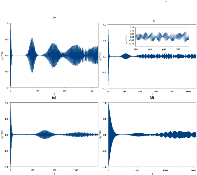
Figure 2: Evolution of the $\langle\hat{\sigma}^{(1)}_{z}(t)\rangle$ against the interaction time $T=\lambda_{1}t$ with $(\alpha,\beta)=(5,5)$ for $(\lambda_{2},\lambda_{3})=(1,0)$ (a), $(1,0.6)$ (b), $(2,3)$ (c) and $(1,1)$ (d).

Now, we comment on the switching mechanism in the AQC. For the sake of comparison, we substitute $\beta=0$ in relations (12)–(34) and calculate the mean-photon numbers as:

$$\begin{array}[]{lr}\langle\hat{a}_{1}^{\dagger}(T)\hat{a}_{1}(T)\rangle=|\alpha|^{2}+\sum\limits_{n=0}^{\infty}|C_{n,0}|^{2}[|X_{3}(T,n,0)|^{2}+|X_{4}(T,n,0)|^{2}],\\ \\ \langle\hat{a}_{2}^{\dagger}(T)\hat{a}_{2}(T)\rangle=\sum\limits_{n=0}^{\infty}|C_{n,0}|^{2}[|X_{2}(T,n,0)|^{2}+|X_{4}(T,n,0)|^{2}],\end{array}$$ (45)

whre $T=t\lambda_{1}$. From these equations it is obvious that the intensity of the mode in the first waveguide cannot be switched to the other one. This is in a clear contrast with the linear directional coupler (compare (2) and (45)). This behavior is related to the nature of the atom-field interaction mechanism, which is close to the classic Lee model of quantum field theory. Moreover, this behavior is still valid even if the interaction between the modes and the atoms in the same waveguide is neglected, i.e. $\lambda_{1}=\lambda_{2}=0$. In this case, expressions (45) exhibit the well-known RCP of the standard JCM eber . The final remark, AQC is able to switch the nonclassical effects from one waveguide to another based on the values of the interaction parameters. This is remarkable from (45), where the mean-photon number in the second waveguide $\langle\hat{a}_{2}^{\dagger}(T)\hat{a}_{2}(T)\rangle$ can exhibit RCP even though the second mode is initially in vacuum state. On the other hand, assume that the mode in the first waveguide is initially prepared in the even coherent state, which can exhibit squeezing, while the second mode is still in vacuum state. In this case, the density matrix of the second mode takes the form:

$$\hat{\rho}_{2}=\sum\limits_{n=0}^{\infty}|C_{2n,0}|^{2}\Bigl{\{}[|X_{1}(T,2n,0)|^{2}+|X_{3}(T,2n,0)|^{2}]|0\rangle\langle 0|+[|X_{2}(T,2n,0)|^{2}+|X_{4}(T,2n,0)|^{2}]|1\rangle\langle 1|\Bigr{\}},$$ (46)

where $|C_{2n}|^{2}$ is the photon-number distribution of the even coherent sate. From (46), squeezing cannot be switched to the second mode. Nevertheless, if the second mode is prepared in the coherent state, it can exhibit squeezing. In this case, the source of the nonclassical effects could be the switching mechanism between the waveguides or the nature of the atom-field interaction.

Now, we use above relations to investigate the atomic inversions and second-order correlation functions in the following section. For the sake of simplicity we consider $\alpha$ and $\beta$ to be real.

III Atomic inversions and second-order correlation function

Atomic inversion of the standard JCM is well known in quantum optics by exhibiting RCP. The RCP has a nonclassical origin and reflects the nature of the statistics of the radiation field. The evolution of the atomic inversion has been realized via, e.g., the one-atom mazer remp and using technique similar to that of the NMR refocusing meu . In this section we investigate the behavior of the AQC by studying the evolution of the atomic inversions and the second-order correlation functions. As the system includes two atoms we have two types of the atomic inversion, namely, single atomic inversion and total atomic inversion $\langle\hat{\sigma}_{z}(T)\rangle=\frac{1}{2}[\langle\hat{\sigma}^{(1)}_{z}(T)\rangle+\langle\hat{\sigma}^{(2)}_{z}(T)\rangle]$. From (12) one can obtain the following expressions:

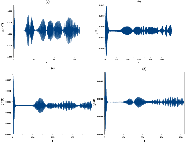
Figure 3: Evolution of the single-mode second-order correlation function as indicated against the interaction time $T=\lambda_{1}t$ with $(\lambda_{2},\lambda_{3})=(1,0)$ (a), $(1,0.6)$ (b), $(2,3)$ (c)–(d).

$$\begin{array}[]{lr}\langle\hat{\sigma}^{(1)}_{z}(T)\rangle=\sum\limits_{n,m=0}^{\infty}|C_{n,m}|^{2}[|X_{1}(T,n,m)|^{2}+|X_{2}(T,n,m)|^{2}-|X_{3}(T,n,m)|^{2}-|X_{4}(T,n,m)|^{2}],\\ \\ \langle\hat{\sigma}^{(2)}_{z}(T)\rangle=\sum\limits_{n,m=0}^{\infty}|C_{n,m}|^{2}[|X_{1}(T,n,m)|^{2}-|X_{2}(T,n,m)|^{2}+|X_{3}(T,n,m)|^{2}-|X_{4}(T,n,m)|^{2}],\\ \\ \langle\hat{\sigma}_{z}(T)\rangle=\sum\limits_{n,m=0}^{\infty}|C_{n,m}|^{2}[|X_{1}(T,n,m)|^{2}-|X_{4}(T,n,m)|^{2}].\end{array}$$ (52)

As we mentioned in the preceding section the conventional directional coupler cannot exhibit RCP in the evolution of the mean-photon numbers. Nevertheless, the standard JCM can exhibit RCP provided that the photon-number distribution of the initial field has a smooth envelope. Similar conclusion has been reported to the two-atom single-mode JCM tess . For the AQC we have found when $\alpha=\beta$ and $\lambda_{j}\neq 0$ the different types of the atomic inversions (52) provide quite similar behaviors. It seems that the contributions of the coherence coefficients $X_{2},X_{3}$ are comparable. Moreover, one can easily prove when $\lambda_{3}=0$ and $\lambda_{1}=\lambda_{2}$ the atomic inversions reduce to that of the standard JCM (see Fig. 2(a)). It is worth reminding that for the standard JCM the revival patterns occur in the atomic inversion over certain period of the interaction time afterward they interfere providing chaotic behavior. Additionally, the revival time is connected with the amplitude $\alpha$ through the relation $T_{r}=2\pi\sqrt{\bar{n}}\simeq 2\pi|\alpha|$ eber . We proceed, for $\lambda_{1}\neq\lambda_{2}$ they provide different forms of the revival patterns. Here we restrict the attention to the atomic inversion of the first atom (see Figs. 2(b)-(d) for the given values of the interaction parameters). We study three cases based on the relationship between the strength of the switching mechanisms in and between the waveguides, namely, $\lambda_{3}<\lambda_{j},\lambda_{3}=\lambda_{j},\lambda_{3}>\lambda_{j}$. Comparisons between Figs. 2(b)-(d) and Fig. 2(a) are instructive. From Fig. 2(b) one can observe that the atomic inversion, after the zero and first revival patterns, exhibits long series of the subsidiary-revival patterns (see the inset in Fig. 2(b)). This behavior is completely different from that of the JCM. This indicates that the nonclassical effects generated by this device can sustain for an interaction time longer than that of the JCM. It is worth mentioning that the subsidiary-revival patterns have been observed for the JCM against the squeezed coherent state eberr1 . This has been explained in relation to the photon-number distribution of the initial states. More illustratively, the photon-number distributions of the squeezed states exhibit many peaks structure, each of which gives its own revival patterns in the evolution of the atomic inversion. These patterns interfere with each other to produce these subsidiary-revival patterns. Nevertheless, for the system under consideration the occurrence of these patterns is related to the switching mechanism between the waveguides (compare Figs. 2(a) and (b)). This mechanism reflects itself in very complicated Rabi oscillations $\Omega_{\pm}$ as well as in the double summations in the atomic inversions formulae (52). Fig. 2(c) presents the case when the coupling constants are different. It is obvious that the RCP is still remarkable and the subsidiary revivals are smoothly washed out compared to those in Fig. 2(b). Generally, we have found when $\lambda_{3}\geq\lambda_{1}=\lambda_{2}$ the atomic inversion exhibits long RCP (see Fig. 2(d)). Above information indicates that the switching mechanism between the waveguides plays an important role in the behavior of the AQC. Actually, we have found difficulties in giving mathematical treatment for the RCP presented by the AQC since the Rabi oscillation is rather complicated.

Now we draw the attention to the second-order correlation functions for the single-mode case, which is defined as:

$$g_{j}^{(2)}(t)=\frac{\langle\hat{a}_{j}^{\dagger 2}(t)\hat{a}_{j}^{2}(t)\rangle}{\langle\hat{a}_{j}^{\dagger}(t)\hat{a}_{j}(t)\rangle^{2}}-1,\quad j=1,2,$$ (53)

where $g_{j}^{(2)}(t)=0$ for Poissonian statistics (standard case), $g_{j}^{(2)}(t)<0$ for sub-Poissonian statistics (nonclassical effects) and $g_{j}^{(2)}(t)>0$ for super-Poissonian statistics (classical effects). The second-order correlation function can be measured by a set of two detectors, e.g. the standard Hanbury Brown-Twiss coincidence arrangement. For the system under consideration, this quantity is plotted in Figs. 3 for the given values of the interaction parameters. From these figures it is obvious that the AQC is able to generate long-lived sub-Piossonian effects, i.e. $g_{1}^{(2)}(t)<0$. Furthermore, the basic features of the dynamics are still similar to those of the atomic inversion. Fig. 3(a) presents the well-known shape of the second-order function of the standard JCM. When the switching mechanism between the waveguides is involved the long RCP is dominant in the evolution of the $g_{j}^{(2)}(t)$. Nevertheless, the shape of this phenomenon is quite different from that in the corresponding atomic inversion (compare Fig. 2(b) to Fig. 3(b)). For instance, the revival times in the two quantities are different. Also, the number of the subsidiary revivals in the atomic inversion is greater than that in the corresponding $g_{1}^{(2)}(t)$. In contrast to the atomic inversions, $g_{1}^{(2)}(t)$ and $g_{2}^{(2)}(t)$ can provide different behavior for the same values of the interaction parameters. This fact can be realized by comparing Fig. 3(c) to (d).

In conclusion, in this paper we have developed, for the first time, the notion of the AQC. We have explained how does it work. Also we have derived the exact solution for the equations of motion. In contrast to the conventional coupler the AQC can generate nonclassical effects. Nevertheless, the switching mechanism in the former is more effective than that in the latter. Furthermore, the behavior of the AQC is sensitive to the types of the initial atomic states. We have shown that the system can give the results of the two-mode JCM under certain conditions. Additionally, we have discussed the evolution of the atomic inversions and second-order correlation functions. These two quantities can exhibit RCP, long RCP and long subsidiary-revival patterns based on the values of the coupling constants. Second-order correlation function can exhibit long-lived nonclassical effects. From the information given in the Introduction one can realize that the AQC is in the reach of the current technology. Also it may be of interest in the framework of quantum information.

References

References

- (1) Jensen S M 1982 IEEE J. Quant. Electron. QE 18 1580.
- (2) Nikolopoulos G M 2008 Phys. Rev. Lett. 101 200502.
- (3) Ekert A and Jozsa R 1996 Rev. Mod. Phys. 68 733; Lo H-K, Popescu S and Spiller T 1998 ”Introduction to Quantum Computation and Information” (World Scientific: Singapore); Begie A, Braun D, Tregenna B and Knight P L 2000 Phys. Rev. Lett. 85 1762.
- (4) Kamwa L P, Stitch J E, Mason N J and Roberts P N 1985 Electron. Lett. 21 26; Jin R, Chuang C L, Gibbs H H, Koch S W, Polky J N and Pubanz G A 1986 Appl. Phys. Lett. 49 110.
- (5) Gusovkii D D, Dianov E M, Mairer A A, Neustreuev V B, Shklovskii E I and Scherbakov I A 1985 Sov. J. Quant. Electron. 15 1523.
- (6) Townsend P D, Baker G L, Shelburne J L III and Etemad S 1989 Proc. SPIE 1147 256.
- (7) Peřina Jr J and Peřina J 2000 Progress in Optics 41, ed. E. Wolf (Amsterdam: Elsevier), p. 361.
- (8) Jaynes E T and Cummings F W 1963 Proc. IEEE 51 89.
- (9) Bose S, Fuentes-Guridi I, Knight P L and Vedral V 2001 Phys. Rev. Lett. 87 050401.
- (10) Eberly J H, Narozhny N B and Sanchez-Mondragon J J 1980 Phys. Rev. Lett. 44 1323; Narozhny N B, Sanchez-Mondragon J J and Eberly J H 1981 Phys. Rev. A 23 236; Yoo H I, Sanchez-Mondragon J J and Eberly J H 1981 J. Phys. A 14 1383; Yoo H I and Eberly J H 1985 Phys. Rep. 118 239.
- (11) El-Orany F A A and Obada A-S 2003 J. Opt. B: Quant. Semiclass. Opt. 5 60.
- (12) Rempe G, Walther H and Klein N 1987 Phys. Rev. Lett. 57 353.
- (13) Meunier T, Gleyzes S, Maioli P, Auffeves A, Nogues G, Brune M, Raimond J M and Haroche S 2005 Phys. Rev. Lett. 94 010401.
- (14) Yeazell J A, Mallalieu M and Stroud C R Jr 1990 Phys. Rev. Lett. 64 2007; Brune M, Schmidt-Kaler F, Maali A, Dreyer J, Hagley E, Raimond J M and Haroche S 1996 Phys. Rev. Lett. 76 1800.
- (15) Vogel W and De Matos Filho R L 1995 Phys. Rev. A 52 4214.
- (16) Meschede D, Walther H and Müller 1985 Phys. Rev. Lett. 54 551; Walther H 1992 Phys. Rep. 219 263.
- (17) Tessier T E, Deutsch I H and Delgado A 2003 Phys. Rev. A 68 062316; Faisal A A El-Orany 2006 J. Phys. A: Math. Gen. 39 3397; Faisal A A El-Orany 2006 Phys. Scripta 74 563.
- (18) Faisal A A El-Orany, Obada A-S F, Abdelslama M A and Wahiddin M R B 2008 J. Mod. Opt. 55 1649.
- (19) Nielsen M and Chuang I 2000 ”Quantum Computation and Quantum Information” (Cambridge University Press, Cambridge); Lambropoulos P and Petrosyan D 2006 ”Fundamentals of Quantum Optics and Quantum Information” (Springer, Berlin).
- (20) Lukin M D 2003 Rev. Mod. Phys. 75 457; Petrosyan D 2005 J. Opt. B 7 S141.
- (21) Noh H-R and Jhe W 2002 Phys. Rep. 372 269.
- (22) Olshanii M A, Ovchinnikov Y B and Letokhov V S 1993 Opt. Comm. 98 77.
- (23) Renn M J, Montgomery D, Vdovin O, Anderson D Z, Wieman C E and Cornell E A 1995 Phys. Rev. Lett. 75 3253.
- (24) Barnett A H, Smith S P, Olshanii M, Johnson K S, Adams A W and Prentiss M 2000 Phys. Rev. A 61 023608.
- (25) Sague G, Vetsch E, Alt W, Meschede D and Rauschenbeutel 2007 Phys. Rev. Lett. 99 163602; Sague G, A Baade A and Rauschenbeutel A 2008 New. J. Phys. 10 113008.
- (26) Nayak K P, Melentiev P N, Morinaga M, Kien F L, Balykin V I and Hakuta K: quant-ph/0610136v1.
- (27) Kien F L, Balykin V I and Hakuta K 2004 Phys. Rev. A 70 063403.
- (28) Dowling J P and Gea-Banacloche J 1996 Adv. At. Mol. Opt. Phys. 37 1.
- (29) Kien F L, Dutta Gupta S, Nayak K P and Hakuta K 2005 Phys. Rev. A 72 063815.
- (30) Horak P, Domokos P and Ritsch H 2003 Europhys. Lett. 61 459.
- (31) Abdel-Aty M, Abdalla M S and Sanders B C 2009 Phys. Let. A 373 315.
- (32) Janszky J, Sibilia C, Bertolotti M and Yushin Y 1988 J. Mod. Opt. 35 1757.
- (33) Louisell W H ”Quantum Statistical Properties of Radiation” (New York: Wiley 1973).
- (34) Yöna M, Ting Y and Eberly J H 2007 J. Phys. B: At. Mol. Opt. Phys. 40 S45-S59.
- (35) Casagrande F, Lulli A, and Paris M G A 2007 Phys. Rev. A 75 032336.
- (36) Jozsa R, Abrams D S, Dowling J P and Williams C P 2000 Phys. Rev. Lett. 85 2010.
- (37) Gerry C C and Eberly J H 1990 Phys. Rev. A 42 6805; Cardimona D A, Kovanis V, Sharma M P and Gavrielides A 1991 Phys. Rev. A 43 3710.
- (38) Satyanarayana M V, Rice P, Vyas R and Carmichael H J 1989 J. Opt. Soc. Am. B 6 228.