Type II Supernovae: Model Light Curves and Standard Candle Relationships

Abstract

A survey of Type II supernovae explosion models has been carried out to determine how their light curves and spectra vary with their mass, metallicity and explosion energy. The presupernova models are taken from a recent survey of massive stellar evolution at solar metallicity supplemented by new calculations at sub-solar metallicity. Explosions are simulated by the motion of a piston near the edge of the iron core and the resulting light curves and spectra are calculated using full multi-wavelength radiation transport. Formulae are developed that describe approximately how the model observables (light curve luminosity and duration) scale with the progenitor mass, explosion energy, and radioactive nucleosynthesis. Comparison with observational data shows that the explosion energy of typical supernovae (as measured by kinetic energy at infinity) varies by nearly an order of magnitude – from $0.5$ to $4.0~{}\times 10^{51}$ ergs, with a typical value of $\sim 0.9\times 10^{51}$ ergs. Despite the large variation, the models exhibit a tight relationship between luminosity and expansion velocity, similar to that previously employed empirically to make SNe IIP standardized candles. This relation is explained by the simple behavior of hydrogen recombination in the supernova envelope, but we find a sensitivity to progenitor metallicity and mass that could lead to systematic errors. Additional correlations between light curve luminosity, duration, and color might enable the use of SNe IIP to obtain distances accurate to $\sim$20% using only photometric data.

1. Introduction

Type II supernovae (SNe II) result from the explosion of massive stars that have retained their hydrogen envelope until their cores collapse to neutron stars or black holes. The most common events, the Type II plateau supernovae, have a distinctive light curve, maintaining a nearly constant luminosity for $\sim 100$ days, then suddenly dropping off. Upcoming synoptic surveys should discover millions of these events out to redshifts of a few. These observations will probe massive stellar evolution in a broad range of galactic environments, and may also be used to measure cosmological distances and test host galaxy dust properties.

SNe II are diverse transients in terms of their luminosities, durations, and expansion speeds. By modeling the observed light curves and spectra, one can constrain the physical properties of the explosion such as the ejected mass, explosion energy, and presupernova radius. In a pioneering study, Hamuy (2003) analyzed 16 observed supernovae and derived masses between $15$ and $50~{}{\mathrm{M}_{\odot}}$ and presupernova radii ranging from $70$ to $600~{}$R_⊙. Unfortunately these inferred values seem implausible, especially the high masses. Direct observations of the progenitors of nearby SNe II from pre-explosion images indicate masses of only $8-15~{}{\mathrm{M}_{\odot}}$ (Smartt et al., 2008), while modern stellar evolution models predict a mass range of $\sim 12-25$ $\mathrm{M}_{\odot}$ (e.g., Woosley et al., 2002; Woosley & Heger, 2007). The overly large values inferred by Hamuy (2003) likely reflect deficiencies in the theoretical models used in the light curve analysis (Litvinova & Nadezhin, 1985). More recent models tailored to individual events have returned more reasonable numbers (e.g. Utrobin & Chugai, 2008; Baklanov et al., 2005).

Observations of SNe II are also used to measure cosmological distances. In terms of brightness alone, they are poor standard candles with luminosities varying by more than an order of magnitude, but various methods can be used to standardized them. Most previous studies were of the Baade-Wessellink type, e.g., the expanding photosphere method (Kirshner & Kwan, 1974; Eastman et al., 1996; Dessart & Hillier, 2005a; Dessart et al., 2008; Jones et al., 2009) and the spectral-fitting expanding atmosphere method (SEAM, Mitchell et al., 2002; Baron et al., 2004). Both approaches require detailed atmospheric modeling. More recently, Hamuy & Pinto (2002) suggested a much simpler approach using an empirical correlation between plateau luminosity and expansion velocity (as measured from the Doppler shift of spectral lines). This standardized candle method has been extended out to moderate redshifts with promising results (Nugent et al., 2006; Poznanski et al., 2008). However, the physical underpinnings of the method and its potential vulnerability to systematic error have not yet been fully explored.

Here we present a new survey of SNe IIP models based on the one-dimensional explosion of realistic progenitor star models of various masses, metallicities, and explosion energies. We calculate the broadband light curves and the detailed spectral evolution using a code that includes a full multi-wavelength solution to the radiation transport problem. The models allow us to explore the light curves dependence on model parameters, which we compare to analytic expectations. We also reproduce and illuminate the physics leading to the standardized candle relation.

2. Analytical Scalings

Some insight into the light curves of SNe IIP can be gained from analytical scalings which express how the observables – luminosity, $L_{\rm sn}$, light curve duration, $t_{\rm sn}$, and expansion velocity, $v_{\rm sn}$– depend on the basic supernova parameters – the explosion energy, $E$, ejecta mass, $M_{\mathrm{ej}}$ and presupernova radius, $R_{0}$. Although the analytic light curves themselves are only approximate, the scaling relations can be quite accurate (Arnett, 1980; Chugai, 1991; Popov, 1993). As a guide to the model results below, we rederive here some basic results using simple physical arguments.

Although the mechanism of core-collapse supernova explosions is complicated, the end result is the deposition of order $E\sim 10^{51}~{}{\rm ergs}=1$ B near the center of the star, and subsequently, the propagation of a blast wave that heats and ejects the stellar envelope. At the time the shock reaches the surface (hours to days), the explosion energy is roughly equally divided between internal and kinetic energy. In the hydrogen envelope, radiation energy dominates the thermal energy of ions and electrons by several orders of magnitude.

In the subsequent expansion, the internal energy is mostly converted into kinetic. The ejecta is optically thick to electron scattering, and the adiabatic condition gives $E_{\rm int}(t)=E_{0}(R(t)/R_{0})^{-1}$, where $E_{0}\approx E/2$ is the initial internal energy, and $R$, the radius. After many doubling times, the ejecta reaches a phase of free homologous expansion, where the velocity of a fluid element is proportional to radius $R=vt$. The final velocity of the ejecta is of order

$$v_{\rm sn}\approx(2E/M_{\mathrm{ej}})^{1/2}=3\times 10^{8}~{}M_{10}E_{51}~{}{\rm cm~{}s}^{-1},$$ (1)

where $M_{10}=M_{\mathrm{ej}}/10~{}{\mathrm{M}_{\odot}}$, $E_{51}=E/10^{51}$ ergs. For homologous expansion, the internal energy evolves as $E_{\rm int}(t)=E_{0}(t/t_{e})^{-1}$ where $t_{e}=R_{0}/v_{\rm sn}$ is the expansion time. Dimensionally, the luminosity of the light curve will then be

$$L_{\rm sn}=\frac{E_{\rm int}(t_{\rm sn})}{t_{\rm sn}}=\frac{E_{0}t_{e}}{t_{\rm sn}^{2}},$$ (2)

where $t_{\rm sn}$ is the appropriate timescale for the duration of the light curve. We determine $L_{\rm sn}$ and $t_{\rm sn}$ below for three different scenarios.

First, if the opacity, $\kappa$, in the supernova envelope were a constant, the time scale of the light curve would be set by the effective diffusion time. Given the mean free path $\lambda_{p}=(\kappa\rho)^{-1}$ and the optical depth of the ejecta $\tau=R/\lambda_{p}$, the diffusion time is

$$t_{\rm sn}=\tau^{2}\frac{\lambda_{p}}{c}=\frac{R^{2}\kappa\rho}{c}.$$ (3)

Over time, the supernova radius increases and the density decreases due to the outward expansion. Using the characteristic values $R(t_{\rm sn})=v_{\rm sn}t_{\rm sn}$ and $\rho(t_{\rm sn})\sim M_{\mathrm{ej}}/R(t_{\rm sn})^{3}$ in Eq. 3, one can solve for $t_{\rm sn}$.

$$\begin{split}t_{\rm sn}&\propto E^{-1/4}M_{\mathrm{ej}}^{3/4}\kappa^{1/2}\\ L_{\rm sn}&\propto E~{}M_{\mathrm{ej}}^{-1}R_{0}~{}\kappa^{-1},\end{split}$$ (4)

where the scaling for $L_{\rm sn}$ was determined by using $t_{\rm sn}$ in Eq. 2. These are the scalings of Arnett (1980)

The results Eq. 4, though commonly applied, are not quite adequate for SNe IIP because the assumption of constant opacity neglects the important effects of ionization (Grassberg et al., 1971). Once the outer layers of ejecta cool below $T_{\rm I}\approx 6000$ K, hydrogen recombines and the electron scattering opacity drops by several orders of magnitude. A sharp ionization front develops – ionized material inside the front is opaque, while neutral material above the front is transparent. The photon mean free path in the ionized matter ($\lambda_{\rm mfp}\sim 10^{10}$ cm) is much smaller than the ejecta radius ($R=v_{\rm s}t\approx 10^{15}$ cm), so the supernova photosphere can be considered nearly coincident with the ionization front.

As radiation escapes and cools the photosphere, the ionization front recedes inward in Lagrangian coordinates, in what is called a recombination wave. The progressive elimination of electron scattering opacity allows for a more rapid release of the internal energy. Once the ionization front reaches the base of the hydrogen envelope, and the internal energy has been largely depleted, the light curve drops off sharply, ending the “plateau”. Any subsequent luminosity must be powered by the decay of radioactive elements synthesized in the explosion (the light curve “tail”).

To account for hydrogen recombination while ignoring, for the moment, radiative diffusion (as in Woosley, 1988; Chugai, 1991), we use the fact that the photosphere is fixed near the ionization temperature $T_{\rm I}$ and radiates a luminosity $L_{p}$ given by

$$L_{p}=4\pi R^{2}\sigma T_{\rm I}^{4}$$ (5)

The light curve timescale $t_{\rm sn}$ is then given by how long it takes the photosphere to radiate away all of the (adiabatically degraded) internal energy – in other words, $L_{p}t_{\rm sn}=E_{0}(t_{e}/t_{\rm sn})$. This, (along with $R=v_{s}t_{\rm sn}$) gives

$$\begin{split}t_{\rm sn}&\propto E^{-1/8}M_{\mathrm{ej}}^{3/8}R_{0}^{1/4}T_{\rm I}^{-1},\\ L_{\rm sn}&\propto E^{3/4}M_{\mathrm{ej}}^{-1/4}R_{0}^{1/2}T_{\rm I}^{2}.\end{split}$$ (6)

Unlike Eqs. 4, these scalings show no dependence on $\kappa$. Effectively, the assumption is that the ejecta is infinitely opaque below the recombination front, and fully transparent above. We will see in the numerical models that this assumption is not totally correct, and hence diffusion below the photosphere is important.

Finally, to derive scalings which include both the effects of radiative diffusion and recombination (as in Popov, 1993), we return to the diffusion time equation of Eq. 3, but now realize that the radius of the opaque debris changes over time, not only due to the outward expansion but also from the inward propagation of the recombination front. This photospheric radius is determined from Eq. 5

$$R_{i}^{2}=\frac{L_{p}}{4\pi\sigma T_{i}^{4}}=\frac{E_{0}t_{e}}{t_{\rm sn}^{2}4\pi,\sigma T_{i}^{4}}$$ (7)

where in the last equality we used Eq. 2 to rewrite $L_{p}=L_{\rm sn}$. Plugging this expression for the radius into the numerator of Eq. 3 gives

$$\begin{split}t_{\rm sn}&\propto E^{-1/6}M_{\mathrm{ej}}^{1/2}R_{0}^{1/6}\kappa^{1/6}T_{\rm I}^{-2/3}\\ L_{\rm sn}&\propto E^{5/6}M_{\mathrm{ej}}^{-1/2}R_{0}^{2/3}\kappa^{-1/3}T_{\rm I}^{4/3}.\end{split}$$ (8)

These scalings are identical to those found by Popov (1993) in a more involved analysis.

So far, the light curves described have only accounted for shock deposited energy. Radioactive ${}^{56}\mathrm{Ni}$ synthesized in the explosion introduces an additional energy source concentrated near the center of the debris. The heating from radioactive decay helps maintain the ionization of the debris and so extends the duration of the plateau. To incorporate this effect into the scalings, we generalize the expression for the internal energy

$$E_{\rm int}(t)=E_{0}\frac{t_{e}}{t}+E_{\rm ni}\frac{t_{\rm ni}}{t}+E_{\rm co}\frac{t_{\rm co}}{t},$$ (9)

where $E_{\rm ni}\approx 0.6\times 10^{50}M_{\mathrm{Ni}}$ ergs, $E_{\rm co}\approx 1.2\times 10^{50}M_{\mathrm{Ni}}$ ergs are the total energy released from ${}^{56}\mathrm{Ni}$ and ${}^{56}\mathrm{Co}$ decay (with $M_{\mathrm{Ni}}$ in units of $\mathrm{M}_{\odot}$) and $t_{\rm ni}\approx 8.8,t_{\rm co}\approx 113$ days are the lifetimes. This correction for radioactivity can be written $E_{\rm int}(t)=E_{0}(t_{e}/t_{\rm sn})f_{\rm rad}$ with

$$f_{\rm rad}=1+0.26\frac{M_{\mathrm{Ni}}}{E_{51}}\frac{t_{\rm co}}{t_{e}},$$ (10)

where $E_{51}=E/10^{51}$ ergs. Following the same arguments leading to Eq. 8, we see that the plateau timescale scales as $t_{\rm sn}\propto f_{\rm rad}^{1/6}$. For example, a ${}^{56}\mathrm{Ni}$ mass of $0.1~{}{\mathrm{M}_{\odot}}$ should extend the plateau by $\sim 24\%$ for $E_{51}=1$. Although one might anticipate a change to $L_{\rm sn}$ as well, the models show that the decay energy does not typically have enough time to diffuse out and affect the plateau luminosity (see Section 6).

Below we compare the analytic scalings to our numerical simulations and show that the simple relations, particularly Eqs. 8, agree quite well. The models allow us to refine the exponents and calibrate the numerical constants in front.

3. Progenitor Models

Table 1Progenitor Star Models

$M_{\rm i}$	$Z$	$M_{\rm f}$	$R_{0}$	$M_{\rm Fe}$	$X_{He}$
12	1.0	10.9	625	1.365	0.30
15	1.0	12.8	812	1.482	0.33
15	0.1	13.3	632	1.462	0.33
20	1.0	15.9	1044	1.540	0.38
25	1.0	15.8	1349	1.590	0.45

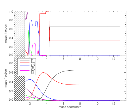
Figure 1.— Abundance distribution of model M15_E.12 after explosion assuming either no mixing (top panel) or the mixing applied in this paper (bottom panel). The inner hashed region form the remnant..

For our numerical models, we consider stellar progenitors with main sequence masses in the range $M_{\rm i}=12-25~{}{\mathrm{M}_{\odot}}$, the range expected to produce most of the observed events. Properties of the presupernova models are summarized in Table 1 which gives the zero age main sequence and presupernova masses in solar masses ($M_{\rm i}$ and $M_{\rm f}$), the presupernova radius in solar radii ($R_{0}$), the iron core mass in solar masses ($M_{\rm Fe}$), and the surface helium mass fraction. All models were computed with the Kepler code, which follows stellar evolution including the most up-to-date opacities, prescriptions for mass loss, and nuclear reaction rates (Rauscher et al., 2002; Woosley et al., 2002; Woosley & Heger, 2007). Stars with larger initial masses experience more mass loss, especially during the red giant phase,and this narrows the range of final masses to $M_{\rm f}=10.9-15.8$ $\mathrm{M}_{\odot}$. For $M_{\rm i}>20~{}{\mathrm{M}_{\odot}}$, the presupernova mass declines with increasing $M_{\rm i}$. More massive stars do, however, maintain significantly larger radii at the time of explosion.

The helium mass fraction in the stellar envelope is also a function of $M_{\rm i}$ (Table 1) varying from 30% for $M_{\rm i}=12$ $\mathrm{M}_{\odot}$ to 45% for $M_{\rm i}=25~{}{\mathrm{M}_{\odot}}$. This variation is due to mass loss and convective dredge up from the helium core, which are greater in more massive stars. As the envelope helium abundance affects both the electron scattering opacity and the recombination temperature of the ejecta, we will find it has a significant effect on the light curves of SNe IIP.

While most stars in our survey have solar abundances, a lower metallicity ($Z=0.1$ solar) $15~{}{\mathrm{M}_{\odot}}$ model was also included. The chief effect of the lower metallicity was a smaller presupernova radius and less total mass loss.

4. Explosions and Nucleosynthesis

4.1. Mass Cut, Fallback, and the Production of ${}^{56}\mathrm{Ni}$

The explosion of each model was simulated by moving a piston outward from an inner boundary at mass coordinate $M_{\rm pist}$ (Woosley & Weaver, 1995; Woosley et al., 2002), typically taken to be the outer edge of the iron core, and following the subsequent hydrodynamics assuming radial symmetry. Each star was exploded several times to obtain variable kinetic energies at infinity within the set of approximately $0.3,0.6,1.2,2.4$, and $4.8\times 10^{51}$ erg. The results are summarized in Table 2. Polarization observations of SNe IIP suggest that the hydrogen envelopes are indeed spherically symmetric, although the cores may appear aspherical, perhaps due to an asymmetric explosion mechanism (Leonard et al., 2006, 2001). Any asymmetry in the shock wave, however, is likely smoothed out by propagating through the large hydrogen envelope.

Explosive nucleosynthesis was calculated using the same code and physics as in Woosley & Heger (2007). While the mass of ${}^{56}\mathrm{Ni}$ that is synthesized is numerically well determined by this procedure, it is an overestimate for two reasons. First, situating the piston at the edge of the iron core, the deepest it can possibly be without violating nucleosynthetic constraints on the iron isotopes, overestimates both the density and mass close to the explosion. It is difficult to launch a successful explosion in the face of such high accretion and a more reasonable location for the piston might be farther out near the base of the oxygen shell. There is a sudden increase in the entropy per baryon, $S/N_{A}k$, to a value around 4.0 signals a rapid fall off in density in the presupernova star. To illustrate the sensitivity to the piston location, a second version of the 0.6 B explosion of the solar metallicity 15 $\mathrm{M}_{\odot}$ star was calculated with the piston at the location where $S/N_{A}k$ = 4.0. The ${}^{56}\mathrm{Ni}$ production declined from 0.24 $\mathrm{M}_{\odot}$ to 0.084 $\mathrm{M}_{\odot}$.

Second, the ejection of ${}^{56}\mathrm{Ni}$ is sensitive to the treatment of mixing and fallback. It was assumed here that whatever material had positive speed at 10⁶ s, the time of the link from the Kepler hydrodynamics code to the spectral synthesis code would be ejected. Since some of the slow moving material will fall back into the collapsed remnant at later times, this also overestimates the ejection of ${}^{56}\mathrm{Ni}$. However, mixing which is largely finished before $10^{6}$ s, reduces this sensitivity by taking ${}^{56}\mathrm{Ni}$ that would have fallen in and moving it farther out in the ejecta (Herant & Woosley, 1994; Joggerst et al., 2009).

Observations of the tail of the supernova light curve constrain the mass of ${}^{56}\mathrm{Ni}$ to be in the range $\sim$0.01 - 0.1 $\mathrm{M}_{\odot}$ (Arnett et al., 1989; Smartt et al., 2008) with values closer to 0.1 $\mathrm{M}_{\odot}$ coming from the more massive progenitors. All in all, it seems that multiplying the ${}^{56}\mathrm{Ni}$ yield of our models by a factor of $0.25-0.5$ is reasonable. It should be noted that the plateau phase of the light curve is insensitive to the ${}^{56}\mathrm{Ni}$ production (see Section 6).

4.2. Mixing

In addition to its affect on the absolute yields, hydrodynamical mixing during the explosion can carry ${}^{56}\mathrm{Ni}$ out into the hydrogen envelope and hydrogen deep into the core of helium and heavy elements. The early appearance of X-rays in SN 1987A and the smoothness of the light curve showed that substantial mixing occurred - more than has been provided so far in any calculation of just the Rayleigh-Taylor instability. Mixing that commences with a broken symmetry in the exploding core itself seems to be necessary (Kifonidis et al., 2003). Because a large number of models needed to be studied here and because the degree of mixing is affected by the uncertain asymmetry of the central engine, we used a simple parametric representation of the mixing similar to that used by Pinto & Woosley (1988) and Heger & Woosley (2008). A running boxcar average of width $\Delta$M is moved through the star a total of $n$ times until the desired mixing is obtained. The default values $\Delta$M and $n$ are 10% of the mass of the helium core and 4, respectively. This gives, for example, the mixed composition for Model 15C in Figure 1.

We explored the effects of varying the degree of mixing, and found that it lead to only small changes at the end of the plateau – i.e. once the recombination wave had reached the inner layers of helium and heavier elements.

5. The Calculation of Light Curves and Spectra

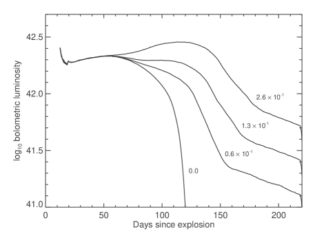
Figure 2.— Bolometric light curves of a standard model (M15_E1.2_Z1) with different amounts of ${}^{56}\mathrm{Ni}$ ejected (marked on figure in units of $\mathrm{M}_{\odot}$). The radioactive energy deposition extends the plateau, but has little impact on the luminosity at $t<50$ days.

Several numerical studies of the light curves of SNe IIP have been published (e.g., Litvinova & Nadezhin, 1985; Young & Branch, 1989; Utrobin, 2007; Nadyozhin, 2003). One common limitation of the previous studies was that the radiative transfer was often treated in the diffusion approximation or with low wavelength resolution, although there have been a few exceptions (c.f., Baklanov et al., 2005; Chieffi et al., 2003). Non-LTE (NLTE) radiative transfer calculations have been applied to the stationary spectra of SNe IIP (e.g., Dessart & Hillier, 2005b; Baron et al., 2003), but not, so far, to time-dependent light curve calculations.

To calculate light curves and spectra of our models, we applied a novel method which coupled a multi-wavelength implicit Monte Carlo radiation transport code to a 1-dimensional hydrodynamics solver (Kasen et al., 2006; Kasen & Woosley, 2009). The initial conditions of the calculation were taken from the Kepler explosion model at $t=10^{6}$ s after explosion. At this time, the ejecta was largely homologous and the hydrodynamics essentially unimportant. While we therefore neglect the earliest part of the light curve, our main interest here is the plateau phase. Detailed radiative transfer calculations of the shock breakout phase and early luminosity will be discussed in a separate paper (Kasen & Woosley, 2009).

In the Monte Carlo approach, the radiation field is represented by discrete photon packets which are tracked through randomized scatterings and absorptions. At the start of the calculation, a large number $(\sim 10^{5}$) of packets were initiated in each zone. The energy of the packets was chosen so that the sum equaled the equilibrium radiation energy of the zone. The initial frequency $\nu$ and direction vector $\hat{D}$ of each packet were sampled assuming that the distribution was isotropic and blackbody in the comoving frame. Throughout the simulation, additional packets were created to model gamma-rays input by the decay of ${}^{56}\mathrm{Ni}$ and ${}^{56}\mathrm{Co}$. The transport and absorption of these gamma rays were likewise followed using a Monte Carlo approach applying the relevant opacities.

We adopted a mixed-frame approach for the transport whereby the gas opacities and emissivities were calculated in the comoving frame, while Monte Carlo packets were tracked in the lab frame. The relevant optical opacities included electron scattering, bound-free, free-free, and bound-bound line opacity, the last treated in the expansion opacity formalism of Eastman & Pinto (1993). The matter ionization and excitation state were computed assuming Saha/Boltzmann statistics at the matter temperature. While the code allows for non-equilibrium between matter and radiation temperatures, the radiation energy density is so dominant in SNe IIP that the two equilibrated on a short timescale.

The scattering of photon packets was simulated by Lorentz transforming a packet into the comoving frame, preforming an isotropic scattering, and then transforming back to the lab frame. The application of the two Lorentz transformations changes the energy and frequency of the outgoing packet. When averaged over many scattering events, this effect accounts for the work done by the radiation field. We checked that the correct behavior was recovered in very optical thick regions of the ejecta, where the radiation energy density evolved with time as it should for a homologous adiabatic flow, $e_{rad}\propto(t/t_{0})^{-4}$.

While the properties of individual packets were sampled from continuous distributions in space, time, and wavelength, the grid through which they moved was discrete. In these calculations, the ejecta was divided into 150 equally spaced radial zones. Opacities and emissivities in each zone were further defined on a wavelength grid of range $1-25,000$ Å with a constant binning of 5 Å. The physical properties of the zones (e.g., density, temperature, ionization state, and opacity) were updated on a timescale chosen much shorter than the dynamical timescale, with time-steps not exceeding $5\times 10^{4}$ s. Higher resolution tests were performed to confirm that the discretization was adequate.

NLTE calculations of Type II spectra show that deviations from LTE have significant effects on line profiles, while the continuum flux is less affected (Baron et al., 1996; Dessart & Hillier, 2008). To estimate the potential effects, we computed stationary NLTE spectra on the plateau (day 50 after explosion) using the same code. A particularly relevant NLTE effect is on the Ca II IR-triplet, whose emission is over predicted by LTE enough to cause a $\sim 0.1$ mag increase in $I$-band magnitude. While still relatively small, this error could be significant when using the predicted $V-I$ color to correct for dust extinction in observations. We therefore used the NLTE spectral results for the discussion in Section 8. Time-dependent NLTE effects, which are not included here, can strongly affect the emission in the hydrogen Balmer lines (Dessart & Hillier, 2008) and the H-alpha line in particular, which would modify the $R$-band magnitudes.

6. A Typical Model

6.1. Bolometric Light Curve

Figure 3.— Evolution of the hydrogen ionization fraction over time for model M15_E1.2_Z1. The ejecta photosphere forms near the ionization front, which recedes inward in velocity (i.e., Lagrangian) coordinates as the photosphere radiates and cools. The plateau ends when the ionization front reaches the base of the hydrogen front.

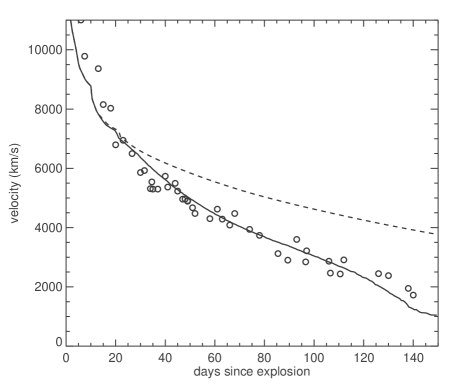
Figure 4.— Photospheric velocity evolution of model M15_E1.2_Z1 as a function of time. The solid line shows the velocity of the electron scattering photosphere defined at $\tau_{e}=2/3$. The dashed line shows the photospheric velocity in a model in which hydrogen recombination is neglected. The circles are the observed velocities of the sample of SNe IIP compiled by Nugent et al. (2006)

We first focus on the properties of a typical SNe IIP model (M15_E1.2_Z1) which has parameters thought to be common: $M_{\rm i}=15~{}{\mathrm{M}_{\odot}},E=1.2$ B, and solar metallicity. Figure 2 shows the bolometric light curve for different values of the ejected ${}^{56}\mathrm{Ni}$ mass. Initially, the model luminosity decreases after shock breakout, and reaches a minimum around day 20. At that time, the outermost layers of ejecta become cool enough such that hydrogen can recombine. This might be considered the beginning of the plateau phase.

On the plateau, the position of the photosphere is determined by the location of the hydrogen recombination front, which occurs at a temperature $T_{\rm I}\approx 6000$ K. As the ejecta cool, the front recedes inward (Figure 3). At around day 120, the front reaches the base of the hydrogen envelope. Recombination occurs more quickly in the helium layers, so the remaining internal energy is depleted quickly and the light curve drops off sharply, ending the plateau.

The evolution of the photospheric velocity over time (Figure 4) agrees well with the observations of SNe IIP compiled by Nugent et al. (2006). Had we ignored the effects of hydrogen recombination, the photospheric velocity would have declined much more slowly, in conflict with the observed. Thus, although the photospheric velocity is often taken as a measure of $(E/M_{\mathrm{ej}})^{1/2}$ (i.e., Eq. 1) for SNe IIP this is clearly only valid for times before recombination sets in (here $t\lesssim 20$ days). At later times, the position of the photosphere is largely determined by the inward progression of the recombination front.

Figure 6 further illustrates how the nature of the opacity affects the light curve. If we artificially increase the electron scattering opacity by a factor of 2, the light curve becomes dimmer and broader, in agreement with the analytical scalings of Eq. 8. This indicates that radiative diffusion in the ionized regions is indeed significant. If we neglect the effects of hydrogen recombination, the resulting light curve declines in a roughly power law fashion, with a lower average luminosity and longer duration. This implies that the recombination wave is responsible for the flatness of the plateau and the steep drop off afterward.

The opacity is also affected by the helium abundance $X_{\rm he}$ in the hydrogen envelope. Because helium recombines at higher temperatures than hydrogen, a larger $X_{\rm he}$  effectively reduces the electron scattering opacity. The light curve of a model with $X_{\rm he}=0.5$ is therefore $0.4$ mag brighter and 20 days shorter than one assuming pure hydrogen (Figure 7). Helium in the core of the ejecta also affects the light curve, though in a slightly different way. For models with larger helium cores, the recombination front will reach the base of the hydrogen layer at an earlier time, and so the plateau will end relatively sooner.

As expected from the analytical arguments of Section 2, the inclusion of radioactive ${}^{56}\mathrm{Ni}$ extends the plateau duration, but has essentially no effect on the luminosity at times $\lesssim 50$ days (Figure 2). Because ${}^{56}\mathrm{Ni}$ is synthesized only at the ejecta center, radioactive energy does not have enough time to diffuse out and affect the plateau unless extreme masses or outward mixing of ${}^{56}\mathrm{Ni}$ are considered.

6.2. Broadband Light Curves and Spectra

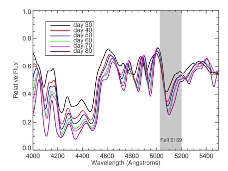
Figure 5.— Evolution of the Fe II and Ti II lines in the spectral range 4000-5550 Å. The recession of the photosphere is observable in the decreasing Doppler shift of the line minima, especially that of Fe II $\lambda 5169$ line.

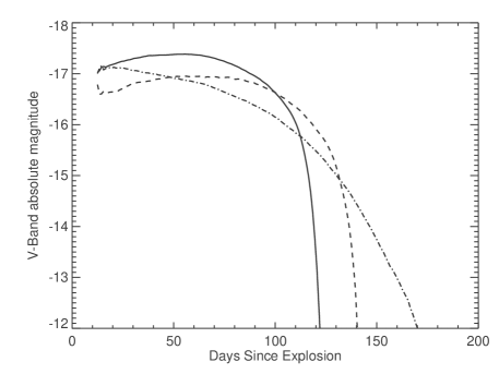
Figure 6.— V-band light curve of model M15_E1.2_Z1 (with no ${}^{56}\mathrm{Ni}$ included) computed using different opacity prescriptions. The solid line properly includes all relevant opacities. The dash-dotted line shows a model in which hydrogen is not allowed to recombine, which demonstrates the importance of ionization effects on the plateau. The dashed line shows a model in which the electron scattering opacity was increased by a factor of 2, which demonstrates the importance of diffusion in the ionized regions.

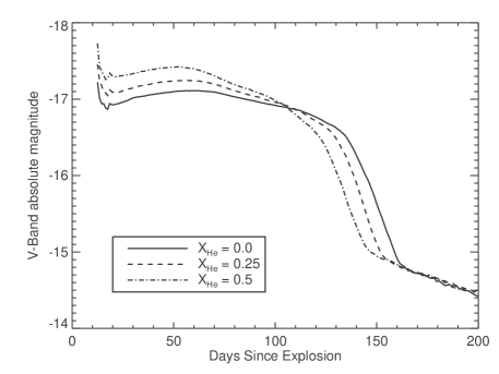
Figure 7.— Bolometric light curves of model M15_E1.2_Z1 (with a ${}^{56}\mathrm{Ni}$ mass of $0.06~{}{\mathrm{M}_{\odot}}$) computed with different helium abundances in the hydrogen envelope. A greater helium abundance reduces the electron scattering opacity and leads to a shorter, brighter plateau.

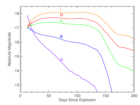
Figure 8.— Broadband UBVRI light curves of our standard model M15_E1.2_Z1 (with an ejected ${}^{56}\mathrm{Ni}$ mass of $0.13~{}{\mathrm{M}_{\odot}}$). The faster decline in the U and B bands is due to increasing line opacity (see Figure 9).

The model broadband light curves are shown in Figure 8. The $U$ and $B$ band light curves decline sharply, showing virtually no plateau, while the $V$, $R$ and $I$ bands are flatter. This behavior, which is also seen in observations, can be understood by examining the spectral evolution on the plateau (Figure 9). At longer wavelengths ($\lambda\gtrsim 5000~{}\AA$) the continuum is fairly well approximated by a blackbody of constant temperature. The $V-I$ and $V-R$ colors are therefore fairly constant over the plateau. At shorter wavelengths ($\lambda\lesssim 5000~{}\AA$) on the other hand, the spectrum is heavily affected by the blanketing from millions of blended iron group lines (in particular those of Fe II and Ti II) reflecting the metallicity of the progenitor star. This line opacity depends sensitively on temperature, as a slight cooling of the photosphere induces Fe III and Ti III to recombine to Fe II and Ti II. The corresponding non-linear increase in line blanketing, clearly visible in Figure 9, causes a drop in $U$ and $B$ magnitudes much greater than would be expected from a pure blackbody spectrum.

Figure 5 illustrates how the inward progression of the supernova photosphere is detectable in the spectral series. The Doppler shifts of Fe II and Ti II absorption lines in the wavelength region 4000-5000 Å decrease over time. In most applications, the Fe II $\lambda 5169$ line is used to infer the photospheric velocity, as it is strong enough to be measured relatively easily, but weak enough to not be saturated above the photosphere.

7. Model Survey

Table 2Properties of Supernova Models

Name	$M_{i}$	$E$	$M_{\rm pist}$	$M_{\mathrm{ej}}$	$M_{\mathrm{Ni}}$	$L_{50}$	$t_{p,0}$	$M_{V,50}$	$v_{ph,50}$
M12_E1.2_Z1	12	1.21	1.36	9.53	0.16	1.91e42	116	-17.25	4915
M12_E2.4_Z1	12	2.42	1.36	9.53	0.18	3.67e42	99	-17.98	6346
M15_E1.2_Z1	15	1.21	1.48	11.29	0.26	2.16e42	124	-17.38	4959
M15_E2.4_Z1	15	2.42	1.48	11.29	0.31	4.35e42	105	-18.15	6491
M15_E0.6_Z1	15	0.66	1.48	11.25	0.24	1.26e42	149	-16.79	3966
M15_E4.8_Z1	15	4.95	1.48	10.78	0.36	7.80e42	88	-18.80	8479
M15_E0.3_Z1	15	0.33	1.48	11.27	0.22	5.93e41	177	-15.96	3125
M20_E1.2_Z1	20	1.22	1.54	14.36	0.34	2.61e42	144	-17.57	4947
M20_E2.4_Z1	20	2.42	1.54	14.37	0.40	4.85e42	119	-18.26	6459
M20_E0.6_Z1	20	0.68	1.54	14.36	0.32	1.40e42	167	-16.89	3979
M20_E4.8_Z1	20	4.99	1.54	14.37	0.48	8.57e42	99	-18.91	8337
M25_E1.2_Z1	25	1.22	1.59	14.22	0.37	3.94e42	131	-18.00	5033
M25_E2.4_Z1	25	2.43	1.59	14.22	0.43	6.66e42	107	-18.59	6483
M25_E0.6_Z1	25	0.66	1.59	14.11	0.34	1.96e42	154	-17.23	4281
M25_E4.8_Z1	25	5.00	1.59	12.97	0.56	1.10e43	86	-19.17	7948
M15_E1.2_Z0.1	15	1.26	1.46	13.27	0.12	1.67e42	130	-17.04	4716
M15_E2.4_Z0.1	15	2.48	1.46	13.24	0.16	3.08e42	107	-17.71	6098
M15_E0.6_Z0.1	15	0.65	1.46	13.28	0.10	8.59e41	156	-16.32	3671
M15_E4.8_Z0.1	15	4.90	1.46	13.18	0.20	5.31e42	88	-18.30	7670

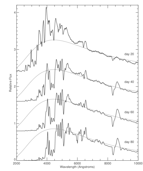
Figure 9.— Spectral evolution of model M15_E1.2_Z1, with the time since explosion marked on the figure. At longer wavelengths ($\lambda\gtrsim 5000~{}\AA$) the spectrum is well approximated by a blackbody at $T\approx 6500$ K (dotted lines). At shorter wavelengths, the iron group line blanketing becomes progressively stronger over time, reducing the flux.

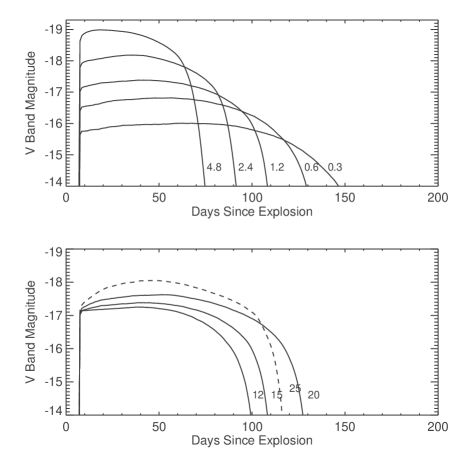
Figure 10.— Model $V$-band light curves from our survey, assuming no ${}^{56}\mathrm{Ni}$ejected. Top: light curves of the $M=15~{}{\mathrm{M}_{\odot}}$ solar metallicity progenitor with different explosion energies (marked on the figure in B). Higher energy explosions are brighter and shorter. Bottom: light curves of 1.2 B explosions with different progenitor initial masses (marked on the figure in $\mathrm{M}_{\odot}$). There is a non-monotonic behavior in the $M=25~{}{\mathrm{M}_{\odot}}$ light curve (dashed line) due to its increased mass loss and envelope helium abundance.

Table 2 and Figures 10 and 11 summarize the light curve properties of the entire model survey. The models vary by more than a factor of 10 in plateau luminosity, and by about a factor of 2 in duration. It is immediately clear that most of the variation in SNe IIP events reflects differences in explosion energy – changes in progenitor mass only account for a factor of $\sim 2$ in luminosity. By directly comparing to the observed sample of nearby SNe IIP (see Section 9), we infer that the explosion energy of real SNe IIP spans the range $0.6-4.8$ B, with a typical mean value around 0.9 B.

Of the analytical scaling laws discussed in Section 2, the model luminosity dependence follows most closely those of Eqs. 8, and in particular $L_{\rm sn}\propto E^{5/6}$. The scaling of the plateau duration, however, deviates from Eqs. 8, following more closely $t_{p}\propto E^{1/4}$. Guided by the analytic results, we find expressions that well fit the models

$$\begin{split}L_{50}&=1.26\times 10^{42}~{}E_{51}^{5/6}M_{10}^{-1/2}R_{0,500}^{2/3}X_{\rm He}^{1}~{}{\rm ergs~{}s}^{-1},\\ t_{p,0}&=122~{}E_{51}^{-1/4}M_{10}^{1/2}R_{0,500}^{1/6}X_{\rm He}^{1/2}~{}{\rm days},\end{split}$$ (11)

where $R_{0,500}=R_{0}/500R_{\odot}$ and $t_{p,0}$ is the plateau duration when no ${}^{56}\mathrm{Ni}$ is included. The $X_{\rm he}$ dependence accounts for the effects of helium both in the envelope and the core. Figure 12 illustrates that the accuracy of these expressions is quite good.

In principle, Eqs. 11 along with the expression for the scaling velocity Eq. 1, could be used to infer the physical parameters $(E,M,R_{0})$ from the observed $(L,t_{p},v)$, in the manner applied by Hamuy (2003). In practice, there are several complicating factors. The envelope helium abundance and the size of the helium core, for instance, are significant factors, but unfortunately there are no clean observables to constrain them. In addition, the photospheric velocity on the plateau is largely determined by recombination, and thus not necessarily a good measure of the ejecta velocity $v_{\rm sn}\propto(E/M_{\mathrm{ej}})^{1/2}$ (see Figure 4). A measurement of the velocity at epochs prior to recombination ($t\lesssim 20$ days) is therefore preferred.

An alternative approach would use the fact that in the progenitor models, $R_{0}$, $M_{ej}$, and $X_{\rm He}$ are correlated, so that some of the degeneracies may be removed. For future photometric surveys, useful relations would allow for a determination of $E$ and $M_{\rm i}$ given only $L_{50}$ and $t_{p,0}$. We find for solar metallicity models

$$\begin{split}L_{50}&=1.49\times 10^{42}~{}E_{51}^{0.82}M_{{\rm in},10}^{0.77}~{}{\rm ergs}\\ t_{p,0}&=128~{}E^{-0.26}M_{{\rm in},10}^{0.11}~{}{\rm days},\end{split}$$ (12)

where $M_{{\rm in},10}=M_{\rm i}/10{\mathrm{M}_{\odot}}$. These relations (which fit the models to within 10%) can be applied to infer the gross properties of SNe IIP without need for follow-up spectroscopy. However, one should bear in mind that they rely on the predictions of stellar evolution and explosion calculations, and thus are subject to uncertainties in, e.g., mass loss and fallback.

Before applying either Eqs. 11 or Eqs. 12 it is critical to account for the fact that ${}^{56}\mathrm{Ni}$ in the ejecta tends to extend the plateau. Figure 13 shows that our derived analytical scaling (Eq. 10) fits reasonably well, with the refined numerical values

$$t_{p}=t_{p,0}\times\biggl{(}1+0.35M_{\mathrm{Ni}}E_{51}^{-1/2}R_{0}^{-1}M_{\mathrm{ej}}^{1/2}\biggr{)}^{1/6}.$$ (13)

We find that the luminosity on the tail of the light curve is nearly identical to the instantaneous energy deposition from ${}^{56}\mathrm{Co}$ decay. The ejected mass of ${}^{56}\mathrm{Ni}$ can then be inferred in the typical way, by measuring the luminosity at a point on the tail. Unfortunately, $M_{\mathrm{ej}}$ and $R_{0}$ also appear in this expression; however, their approximate values for a given initial mass could be taken from Table 1.

8. Bolometric Corrections and Dust

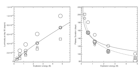
Figure 11.— Light curve properties of all of the models in our survey (assuming no ${}^{56}\mathrm{Ni}$ ejected). Left: bolometric luminosity on the plateau (measured 50 days after explosion) as a function of the explosion energy. Circles denote solar metallicity models, squares $0.1$ solar models, and the size of the symbol is proportional to the progenitor star initial mass. The solid line shows the $L\propto E^{5/6}$ scaling. Right: same as the left panel, but for the plateau duration. The solid line shows the $t_{p}\propto E^{1/6}$ scaling, the dashed line the $t_{p}\propto E^{1/4}$ scaling.

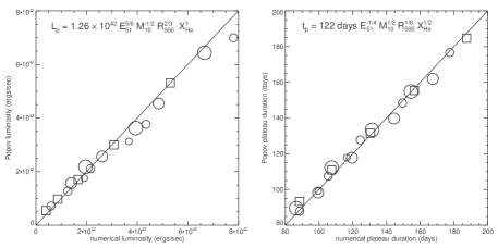
Figure 12.— Accuracy of the analytic scalings Eqs. 8 for the plateau luminosity (left) and duration (right). The $x$-axis values are those determined by the numerical simulation, while the $y$-axis values are those derived from the analytic equation. Circles denote solar metallicity models, squares $0.1$ solar models, and the size of the symbol is proportional to the progenitor star initial mass.

From the models, one can derive formulae useful for making bolometric and dust corrections to observations. Figure 14 plots the difference in bolometric and $V$-band magnitude at day 50 for all models. The typical bolometric corrections are around $0.2$ mag, but increase for brighter events by as much as $0.07$ mag. For solar metallicity models, we fit the relation

$$BC_{50}=0.24-0.025\times(M_{V,50}+18),$$ (14)

where $V_{50}$ is the $V$-band magnitude at day 50. The $Z=0.1$ solar metallicity models, due to the lesser line blocking, have bolometric corrections about $0.07$ mag lower.

Previous studies have typically estimated dust extinction by measuring the $V-I$ excess over an assumed intrinsic color. We find the models have a roughly constant color on the plateau of $V-I\approx 0.5$; however, there is a slight trend for brighter models to be bluer (Figure 15). A fit to the solar metallicity models at day 50 gives

$$(V-I)_{50}=0.52+0.03\times(V_{50}+17.5).$$ (15)

The values are similar to the value $(V-I)_{0}=0.53$ that Nugent et al. (2006) inferred by examining the ridge line of observed events.

As mentioned in Section 5, the model $I$-band magnitudes are sensitive to NLTE effects, especially in the Ca II IR triplet line. Eq. 15 was therefore determined using day 50 spectrum calculations which treated calcium in NLTE, though under the stationary approximation. The model predictions are thus subject to uncertainties in the assumed calcium abundance and perhaps to time dependent NLTE effects (Dessart & Hillier, 2008).

9. Standard Candle Relationship

Figure 13.— Effect of radioactive ${}^{56}\mathrm{Ni}$ on extending the plateau duration. The $y$-axis is the plateau duration $t_{p}$ divided by the $t_{p}$ for the zero ${}^{56}\mathrm{Ni}$ case. The models included here have $M_{\rm i}=15$ $\mathrm{M}_{\odot}$, explosion energies of 1.2 and 2.4 B, and ${}^{56}\mathrm{Ni}$ mass varied from 0 to 0.35 $\mathrm{M}_{\odot}$. The solid line shows the analytic scaling Eq. 13.

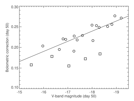
Figure 14.— Bolometric corrections (i.e., bolometric magnitude minus $V$-band magnitude) at day 50 for all models. Circles are solar metallicity models and squares $Z=0.1$ solar model. The dashed line shows a linear fit to the solar metallicity models, Eq. 14.

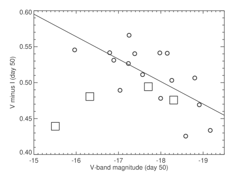
Figure 15.— The $V-I$ color at day 50 for all models. Circles denote solar metallicity models and squares 0.1 solar metallicity models. The solid line shows a linear fit to the solar metallicity models, Eq. 15.

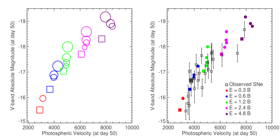
Figure 16.— Model standard candle relationship between the $V$-band plateau luminosity (measured at 50 days) and the photospheric velocity. Left: the models are color coded by explosion energy. Circles denote solar metallicity models, squares $0.1$ solar models, and the size of the symbol is proportional to the progenitor star mass. Right: Comparison of the model relation (circles) with the observation sample compiled by (Hamuy, 2003) (open squares). The large filled square is SN 1999em using the Cepheid distance of Leonard et al. (2003) and an extinction of $A_{v}=0.31$.

Using a sample of nearby observed SN IIP, Hamuy & Pinto (2002) found that the plateau luminosity (measured at day 50 after the explosion) correlated rather tightly with the photospheric velocity, as measured from the Doppler shift of spectral absorption lines. This empirical standard candle (SC) relation provides a simple means for calibrating SN IIP luminosity for distance measures.

Figure 16 shows the Hamuy SC relation for our model survey set, here in terms of the $V$-band magnitude ($M_{V}$) and the photospheric velocity. The model relation is as tight or tighter than the observed, and with a similar slope. The rms dispersion is only $\sigma=0.27$, which translates to $\sim 13\%$ errors in distance measures. To first order, the velocity and luminosity of SNe IIP are both set by the explosion energy. The dispersion in the relation is due to variations in the progenitor mass and metallicity for a given explosion energy.

The physical interpretation of the model SC relation is straightforward, being essentially a recasting of the Baade-Wesselink or expanding photosphere methods that have been in use for many years. The luminosity is written using Stefan’s law and the radius of the supernova photosphere $R=v_{\rm ph}t$

$$L=4\pi v_{\rm ph}^{2}t^{2}\zeta^{2}T_{\rm ph}^{4},$$ (16)

where $\zeta$ is a “dilution” factor which accounts for deviation of the spectrum from blackbody. In Type II atmospheres, both the effects of scattering and line blanketing contribute to $\zeta$ (Wagoner, 1981; Eastman et al., 1996). To determine $L$ using the expanding photosphere method, the observer measures $v_{\rm ph}$ and the time since explosion $t$, and estimates the photospheric temperature $T_{\rm ph}$ from the color of the spectrum. The dilution factor must be calculated using detailed numerical models (the main complexity of the approach). NLTE spectral modeling finds that $\zeta$ varies between 0.5 and 2.0, and is chiefly a function of luminosity, being rather insensitive to other ejecta parameters such as the density structure (Eastman et al., 1996; Dessart & Hillier, 2005a).

The standard candle relation is simply an expression of Eq. 16 under certain restricted conditions. The time since explosion $t$ is, by construction, fixed at 50 days. The temperature $T_{\rm ph}$  for SNe IIP on the plateau is nearly a constant, constrained to be near the recombination temperature $T_{i}\approx 6000$ K. The dilution factor $\zeta$ may vary from event to event, but if $\zeta$ is primarily a function of luminosity this dependence can be absorbed into the exponent. This implies $L=Cv_{\rm ph}^{2+\epsilon}$, where the constant $C$ and the non-blackbody effects $\epsilon$ can be calibrated using a sample of nearby objects, or a set of theoretical models.

The SC relation need not be applied only at day 50, and we find that similar relations apply all along the plateau. However the time since explosion must be known as the normalization depends on time (Eq. 16). We find that an uncertainty in explosion time of 10 days leads to an error in inferred brightness of $0.2-0.3$ mag. It is unwise to apply the SC relation at times much earlier than 30 days, as the ejecta temperatures are likely too high for recombination to have set in, and there is no assurance that $T_{\rm ph}\approx T_{i}$.

One nice feature of the models is that they offer an absolute normalization of the SC relation without needing to assume a value of the Hubble constant. By fitting the relation evaluated at different times since explosion, we find

$$\begin{split}M_{V}(t)=-17.4-6.9\log_{10}(v_{\rm ph}(t)/5000.0)\\ +3.1\log_{10}(t/50~{}{\rm days})\end{split}$$ (17)

The models do predict a deviation from the simple $L\propto v_{\rm ph}^{2}$ relation of Eq. 16, showing instead $L\propto v_{\rm ph}^{2.75}$ in general accordance with that found in the observational sample (Hamuy & Pinto, 2002). This effect is primarily due to the deviation of the spectrum from a blackbody.

The model relation of Figure 16 has a similar normalization to the observations, taken from Hamuy (2003). This implies that our model SC relation is in rough agreement with the distances to SNe IIP obtained in other ways. Particularly comforting is the agreement with SN 1999em, which has a measured Cepheid distance to its host galaxy NGC 1637 of $11.7\pm 1.0$ Mpc (Leonard et al., 2003). We find a very similar distance of $11.6\pm 1.2$ Mpc from Eq. 17 when taking the observed values $m_{v}=13.98$, $v_{\rm ph}=3757~{}\mathrm{km~{}s}^{-1}$, and (following Baron et al., 2000; Hamuy et al., 2001), an extinction of $A_{v}=0.31$. This distance is also consistent with independent estimates using the expanding photosphere method (Dessart & Hillier, 2005a) and SEAM (Baron et al., 2004).

One drawback of the standard candle method, from the observational point of view, is that a high quality spectrum is needed to measure the photospheric velocity – a difficult prospect for high redshift events. As future surveys will observe light curves for a enormous number of SNe IIP with limited spectroscopic follow-up, methods of purely photometric calibration, however coarse, may be of interest. As the explosion energy is the primary variable determining both the plateau luminosity and duration, we explored the relationship between these two observables. A relationship exists (Figure 17) and is fit by

$$M_{V,50}=-18.4-0.03[t_{p,0}-100]$$ (18)

Applying this relation reduces the dispersion from 1 mag down to 0.4 mag. In practice, the measured plateau duration $t_{p}$ must be corrected for the effect of the ejected ${}^{56}\mathrm{Ni}$ mass on its duration in order to determine $t_{p,0}$. The residual scatter in the relation is clearly due to variation in progenitor initial mass or metallicity for a given explosion energy. Presumably, the scatter could be reduced further by using additional light curve relation, such as the color evolution.

10. Discussion and Conclusions

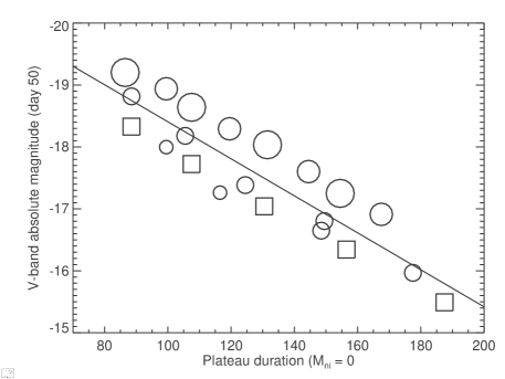
Figure 17.— Relationship between the plateau duration (assuming zero ${}^{56}\mathrm{Ni}$) and the luminosity at day 50. Circles denote solar metallicity models, squares $0.1$ solar models, and the size of the symbol is proportional to the progenitor star mass.

We explored the light curves and spectra of SNe II models with various progenitor masses, metallicities, and explosion energies. We found that explosions with energies $0.3-4.8$ B of stars with initial masses in the range $12-25~{}{\mathrm{M}_{\odot}}$ can explain the observed range of luminosities, velocities, and light curve durations of most SNe IIP. For existing and future observational surveys, the model results should be useful for inferring the progenitor star properties, explosion energies, distances, and dust extinction of observed events.

This study, as have previous studies, quantified how the basic supernova parameters ($M_{\mathrm{ej}}$, $R_{0}$, and $E$) affect the light curves. We also highlighted the important role of two additional parameters: the radioactive ${}^{56}\mathrm{Ni}$ mass and the envelope helium abundance. The presence of ${}^{56}\mathrm{Ni}$ extends the plateau duration, but typically does not affect the luminosity on the plateau at times $t\lesssim 50$ days. The neglect of the effect of ${}^{56}\mathrm{Ni}$ may be the main reason why Hamuy (2003), in his analysis of 16 SNe IIP, inferred implausibly large ejecta masses (up to $50~{}{\mathrm{M}_{\odot}}$). In that study, the longer plateau duration would have to be accounted for by an increased diffusion time, and hence larger ejecta mass. Here we presented analytical formulae which may be useful in accounting for the effects of ${}^{56}\mathrm{Ni}$ on the plateau.

The models confirm the standard candle method of calibrating SNe IIP and illuminate its physical origin. The method is a promising way to determine distances to SNe IIP, with a clear physical explanation in terms of the ionization physics of hydrogen. On the other hand, the models raise some concerns about systematic errors. Progenitors with different masses or metallicities lie on differently normalized relations in Figure 16. If the progenitor population at high redshift has different demographics than that at low redshift (as might be expected) a systematic bias may be introduced into distance measurements. The effect of going from $Z=1$ to $Z=0.1$ solar metallicity in the models is at the 0.1 mag level. It may be possible to reduce these errors by using color information from the light curve.

We find a correlation between plateau luminosity and plateau duration which could be useful in roughly calibrating SNe IIP luminosities using only photometric data (to about 20% in distance). This correlation reflects the fact that in the models one parameter, the explosion energy, primarily controls both the light curve brightness and duration, while the progenitor star properties play a secondary role. The validity of such a relation needs to be empirically checked, as the scatter will be smaller or larger depending on whether the bulk of SNe IIP arise from a narrower or wider range of progenitor masses and radii than that considered here. In practice, the relation also needs to take into account the effect of ${}^{56}\mathrm{Ni}$ on extending the plateau duration.

Correction for dust extinction remains a difficult issue for determining the distances to SNe IIP. The models provide some theoretical guidance as to the intrinsic color evolution of SNe-IIP light curves, however their accuracy may be limited by the assumptions in the radiative transfer, and are sensitive to variations in the envelope metallicity. On the other hand, one could try to invert the problem. Assuming the cosmological parameter are accurately constrained by other means, one could use the standard candle method to solve for the dust extinction of SNe IIP, thus providing an estimate of the variation of dust properties with galactic environment and redshift.

References

- Arnett (1980) Arnett, W. D. 1980, ApJ, 237, 541
- Arnett et al. (1989) Arnett, W. D., Bahcall, J. N., Kirshner, R. P., & Woosley, S. E. 1989, ARA&A, 27, 629
- Baklanov et al. (2005) Baklanov, P. V., Blinnikov, S. I., & Pavlyuk, N. N. 2005, Astronomy Letters, 31, 429
- Baron et al. (2000) Baron, E. et al. 2000, ApJ, 545, 444
- Baron et al. (1996) Baron, E., Hauschildt, P. H., Nugent, P., & Branch, D. 1996, MNRAS, 283, 297
- Baron et al. (2004) Baron, E., Nugent, P. E., Branch, D., & Hauschildt, P. H. 2004, ApJ, 616, L91
- Baron et al. (2003) Baron, E., Nugent, P. E., Branch, D., Hauschildt, P. H., Turatto, M., & Cappellaro, E. 2003, ApJ, 586, 1199
- Chieffi et al. (2003) Chieffi, A., Domínguez, I., Höflich, P., Limongi, M., & Straniero, O. 2003, MNRAS, 345, 111
- Chugai (1991) Chugai, N. N. 1991, Soviet Astronomy Letters, 17, 210
- Dessart et al. (2008) Dessart, L. et al. 2008, ApJ, 675, 644
- Dessart & Hillier (2005a) Dessart, L., & Hillier, D. J. 2005a, A&A, 439, 671
- Dessart & Hillier (2005b) —. 2005b, A&A, 437, 667
- Dessart & Hillier (2008) —. 2008, MNRAS, 383, 57
- Eastman & Pinto (1993) Eastman, R. G., & Pinto, P. A. 1993, ApJ, 412, 731
- Eastman et al. (1996) Eastman, R. G., Schmidt, B. P., & Kirshner, R. 1996, ApJ, 466, 911
- Grassberg et al. (1971) Grassberg, E. K., Imshennik, V. S., & Nadyozhin, D. K. 1971, Ap&SS, 10, 28
- Hamuy (2003) Hamuy, M. 2003, ApJ, 582, 905
- Hamuy & Pinto (2002) Hamuy, M., & Pinto, P. A. 2002, ApJ, 566, L63
- Hamuy et al. (2001) Hamuy, M. et al. 2001, ApJ, 558, 615
- Heger & Woosley (2008) Heger, A., & Woosley, S. E. 2008, ArXiv e-prints
- Herant & Woosley (1994) Herant, M., & Woosley, S. E. 1994, ApJ, 425, 814
- Joggerst et al. (2009) Joggerst, C. C., Woosley, S. E., & Heger, A. 2009, ApJ, 693, 1780
- Jones et al. (2009) Jones, M. I. et al. 2009, ArXiv e-prints
- Kasen et al. (2006) Kasen, D., Thomas, R. C., & Nugent, P. 2006, ApJ, 651, 366
- Kasen & Woosley (2009) Kasen, D., & Woosley, S. 2009, ApJ, in preperation
- Kifonidis et al. (2003) Kifonidis, K., Plewa, T., Janka, H.-T., & Müller, E. 2003, A&A, 408, 621
- Kirshner & Kwan (1974) Kirshner, R. P., & Kwan, J. 1974, ApJ, 193, 27
- Leonard et al. (2001) Leonard, D. C., Filippenko, A. V., Ardila, D. R., & Brotherton, M. S. 2001, ApJ, 553, 861
- Leonard et al. (2006) Leonard, D. C. et al. 2006, Nature, 440, 505
- Leonard et al. (2003) Leonard, D. C., Kanbur, S. M., Ngeow, C. C., & Tanvir, N. R. 2003, ApJ, 594, 247
- Litvinova & Nadezhin (1985) Litvinova, I. Y., & Nadezhin, D. K. 1985, Soviet Astronomy Letters, 11, 145
- Mitchell et al. (2002) Mitchell, R. C., Baron, E., Branch, D., Hauschildt, P. H., Nugent, P. E., Lundqvist, P., Blinnikov, S., & Pun, C. S. J. 2002, ApJ, 574, 293
- Nadyozhin (2003) Nadyozhin, D. K. 2003, MNRAS, 346, 97
- Nugent et al. (2006) Nugent, P. et al. 2006, ApJ, 645, 841
- Pinto & Woosley (1988) Pinto, P. A., & Woosley, S. E. 1988, ApJ, 329, 820
- Popov (1993) Popov, D. V. 1993, ApJ, 414, 712
- Poznanski et al. (2008) Poznanski, D. et al. 2008, ArXiv e-prints
- Rauscher et al. (2002) Rauscher, T., Heger, A., Hoffman, R. D., & Woosley, S. E. 2002, ApJ, 576, 323
- Smartt et al. (2008) Smartt, S. J., Eldridge, J. J., Crockett, R. M., & Maund, J. R. 2008, ArXiv e-prints
- Utrobin (2007) Utrobin, V. P. 2007, A&A, 461, 233
- Utrobin & Chugai (2008) Utrobin, V. P., & Chugai, N. N. 2008, A&A, 491, 507
- Wagoner (1981) Wagoner, R. V. 1981, ApJ, 250, L65
- Woosley (1988) Woosley, S. E. 1988, ApJ, 330, 218
- Woosley & Heger (2007) Woosley, S. E., & Heger, A. 2007, Phys. Rep., 442, 269
- Woosley et al. (2002) Woosley, S. E., Heger, A., & Weaver, T. A. 2002, Reviews of Modern Physics, 74, 1015
- Woosley & Weaver (1995) Woosley, S. E., & Weaver, T. A. 1995, ApJS, 101, 181
- Young & Branch (1989) Young, T. R., & Branch, D. 1989, ApJ, 342, L79