A general method for determining the masses
of semi-invisibly decaying particles at hadron colliders
Konstantin T. Matchev and Myeonghun ParkPhysics Department, University of Florida, Gainesville, FL 32611, USA
(27 December, 2010)
Abstract
We present a general solution to the long standing problem of determining the masses
of pair-produced, semi-invisibly decaying particles at hadron colliders.
We define two new transverse kinematic variables, and ,
which are suitable one-dimensional projections of the contransverse mass
. We derive analytical formulas for the
boundaries of the kinematically allowed regions in the
and parameter planes,
and introduce suitable variables and
to measure the distance to those boundaries on an event per
event basis. We show that the masses can be reliably extracted from the
endpoint measurements of
and (or ).
We illustrate our method with dilepton events at the LHC.
pacs:
14.80.Ly,12.60.Jv,11.80.Cr
The ongoing run of the Large Hadron Collider (LHC) at CERN will finally
provide the first glimpse of physics at the TeV scale.
In large part, the excitement surrounding the LHC is fueled by the
anticipation of the unknown: no one knows for sure where or how
the first signal of new physics beyond the standard model (BSM)
will show up. Yet, complementary and independent
arguments from particle physics and astrophysics
suggest that the best place to look for new physics
is a channel with missing transverse energy ,
caused by unseen new particles contributing to the
dark matter of the Universe.
Unfortunately, the study of missing energy signatures poses
a tremendous challenge at hadron colliders like the LHC.
The first fundamental difficulty is related to the
very nature of hadron colliders,
where in each event the partonic center-of-mass
energy and longitudinal momentum
of the initial state are unknown.
To make matters worse, the lifetime of the dark matter particle
is typically protected by a new parity symmetry,
which guarantees that in every event the missing
particles come in pairs, thus proliferating the number
of unknown parameters describing the final state event
kinematics.
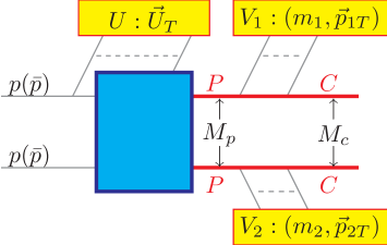
Figure 1:
The generic event topology under consideration.
All particles visible in the detector are clustered into three groups:
upstream objects with total transverse momentum ,
and two composite visible particles (),
each with invariant mass
and total transverse momentum .
The generic topology of a “new physics” event
is sketched in Fig. 1.
Consider the inclusive production of an identical pair of
new “parent” particles . Each parent decays
semi-invisibly to a set ()
of standard model (SM) particles, which are visible in the detector,
and a dark matter particle (from now on referred to as the “child”)
which escapes detection. In general, the parent pair is accompanied by
a number of additional “upstream” objects (typically jets)
with total transverse momentum . They
may originate from various sources such as initial state radiation
or decays of even heavier particles.
We shall not be interested in the exact details of the
physics responsible for , adopting a fully inclusive approach
to the production of the parents . Given this general setup,
the goal is to determine independently the mass of the parent
and the mass of the child in terms of , and .
In the past, several approaches to this problem have been proposed,
but each has its own limitations.
For example, the classic method of invariant
mass endpoints imass; Matchev:2009iw only applies when the visible SM
particles in arise from a sufficiently long decay chain.
Attempts at direct reconstruction exactreco of the
children momenta are again limited to long decay chains only.
In this letter, we shall consider the extreme, most challenging example
where each visible set consists of a single
SM particle of fixed mass . A perfect testing ground
for this scenario is provided by dilepton events
(already observed at the LHC Khachatryan:2010ez)
and we shall use that example in our numerical illustrations below.
The role of the parent (child ) will be played by
the SM -boson (SM neutrino), each is a SM lepton
( or ),
while is composed of the two -jets from the top
quark decays, plus any additional QCD jets from initial
state radiation (ISR).
For such extremely short decay chains, the only viable alternative
at the moment is provided by the methods based
on the variable approxreco.
There, at least in principle,
the individual masses and
can be determined by observing a “kink”
feature in the endpoint as a function
of a hypothesized trial mass for kink,
or by exploring the dependence of the
endpoint Matchev:2009fh.
Compared to those approaches, our method here
has two advantages. First, it is simpler – it
uses only the observed objects , and
in the event and makes no reference to the missing
particle kinematics (or mass).
Second, it is more precise, since it utilizes
the whole kinematic boundary of the relevant
two-dimensional distribution and not just
the kinematic endpoint of its one-dimensional projection.
We proceed in three easy steps.
Step I. Orthogonal decomposition of the
observed transverse momenta with respect to the
direction.
The Tevatron and LHC collaborations currently use
fixed axes coordinate systems to describe their data.
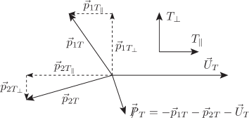
Instead, we propose to rotate the coordinate system
from one event to another, so that the transverse
axes are always aligned with the direction
selected by the measured upstream transverse momentum vector
and the direction orthogonal
to it (see Fig. 2).
The visible transverse momentum vectors from Fig. 1
are then decomposed as
(1)
(2)
Figure 2:
Decomposition of the observed transverse
momentum vectors from Fig. 1 in the transverse plane.
Step II. Constructing the transverse and longitudinal
contransverse masses and .
Our starting point is the original
contransverse mass variable Tovey:2008ui
(3)
where is the “transverse energy” of
(4)
For events with , has an upper endpoint which is
insensitive to the unknown ,
providing one relation among and Tovey:2008ui; Polesello:2009rn
(5)
where
(6)
(7)
Unfortunately, the limit is not particularly interesting
at hadron colliders (especially for inclusive studies),
since a significant amount of upstream is
typically generated by ISR (and other) jets.
One possible fix is to use all events, but
modify the definition (3)
to approximately compensate for the transverse
boost Polesello:2009rn.
One then recovers a distribution whose endpoint is
still given by (5).
Alternatively, one could stick to the original
variable, and simply account for the
dependence of its endpoint as
Our approach here is to utilize the one-dimensional projections
from eqs. (1,2) and construct
one-dimensional analogues of the variable
(10)
(11)
where the corresponding “transverse energies” are
(12)
The benefit of the decomposition (10,11)
is that one gets “two for the price of one”, i.e. two independent and
complementary variables instead of the single variable (3).
The variable in particular
is very useful for our purposes. To illustrate the basic idea,
it is sufficient to consider the most common case,
where is approximately massless (),
as the leptons in our example.
A crucial property of is that its endpoint
is independent of :
(13)
In fact the whole distribution is insensitive to :
(14)
where is the number of events in the zero bin
. Using phase space kinematics,
we find that the shape of the remaining (unit-normalized)
zero-bin-subtracted distribution is simply given by
(15)
in terms of the unit-normalized variable
(16)
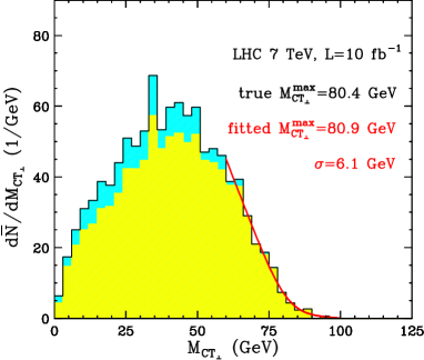
Figure 3: Zero-bin subtracted
distribution after cuts, for
dilepton events. The yellow (lower) portion is our signal,
while the blue (upper) portion shows combinatorial background
with isolated leptons arising from or decays.
The observable distribution for
our example is shown in Fig. 3,
for of LHC data at 7 TeV.
Events were generated with PYTHIA Sjostrand:2006za
and processed with the PGS detector simulator PGS.
We apply standard background rejection cuts as follows
Khachatryan:2010ez: we require two isolated, opposite sign leptons
with GeV, GeV,
and passing a -veto GeV;
at least two central jets with GeV and ;
and a cut of GeV ( GeV) for events with same
flavor (opposite flavor) leptons. We also demand at least
two -tagged jets, assuming a flat -tagging efficiency of .
With those cuts, the SM background from other processes is
negligible Khachatryan:2010ez.
Fig. 3 demonstrates that the
endpoint can be measured quite well. Since the theoretically
predicted shape (15) is distorted by the cuts,
we use a linear slope with Gaussian smearing, and fit
for the endpoint and the resolution parameter.
We find GeV
(compare to the true value GeV),
which gives one constraint (13) among and .
At this point, a second, independent
constraint can in principle be obtained from
an analogous measurement of the
endpoint (8) at a fixed value of
(resulting in loss in statistics), after which the two masses can be found from
(17)
(18)
However, the orthogonal
decomposition (10,11)
offers another approach, which we pursue in the last step.
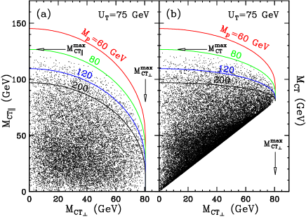
Figure 4:
Scatter plots of (a) versus
and (b) versus , for
a fixed representative value GeV.
The solid lines show the corresponding
boundaries defined in (20)
and (23),
for the correct value of
and several different values of as shown.
Step III. Fitting to kinematic boundary lines.
It is known that two-dimensional correlation plots reveal a lot more
information than one-dimensional projected histograms
boundary; Matchev:2009iw. To this end, consider the scatter plot of
vs in Fig. 4(a),
where for illustration we used 10,000 events at the parton level.
For a given value of ,
the allowed values of are bounded by
(19)
where and
(20)
Fig. 4(a) reveals that the
endpoint
of the one-dimensional
distribution is obtained at
(21)
Notice that events in the zero bins and
fall on one of the axes and cannot
be distinguished on the plot.
Now consider the scatter plot of
vs shown in Fig. 4(b).
is similarly bounded by
(22)
where this time and
(23)
We see that the endpoint of the
one-dimensional distribution
is also obtained for :
(24)
Figure 5: distributions
for four different values of (and given from (18)).
The yellow (light shaded) histograms use
only events in the zero bin
.
The red solid lines show linear
binned maximum likelihood fits.
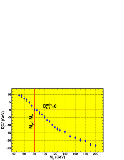
Figure 6: Fitted values of
as a function of .
Fig. 4 reveals a conceptual problem with one-dimensional
projections. While all points in the vicinity of the boundary lines
(20) and (23) are sensitive to the masses,
the endpoint is extracted mostly from
events with ,
while the and
endpoints are extracted mostly from the
events with .
The events near the boundary, but with intermediate values
of , will not enter efficiently either one of these endpoint determinations.
So how can one do better, given the knowledge of the boundary line (23)?
In the spirit of Kim:2009si,
we define the signed distance
to the corresponding boundary,
e.g.
and similarly for .
The key property of this variable is that for the correct values
of and ,
its lower endpoint
is exactly zero (see Fig. 5(b)):
(25)
In that case the boundary line provides a perfectly
snug fit to the scatter plot — notice the green boundary line marked “80” in
Fig. 4(b).
While in general eq. (25)
represents a two-dimensional fit to and , in
practice one can already use the measurement to
reduce the problem to a single degree of freedom, e.g.
the parent mass , as presented in Figs. 4 and
5. We see that the correct parent mass GeV
provides a perfect envelope, for which .
If, on the other hand, is too low, a gap develops between
the outlying points in the scatter plot and their expected boundary,
which results in .
Conversely, if is too high, some of the outlying points
from the scatter plot fall outside the boundary and have ,
leading to , as seen in Fig. 5(c,d).
The resulting fit for as a function of
from our PGS data sample is shown in Fig. 6, which suggests
that a mass measurement at the level of a few percent might be viable.
Acknowledgments.
This work is supported in part by a
US Department of Energy grant DE-FG02-97ER41029.
References
(1)
I. Hinchliffe et al., Phys. Rev. D 55, 5520 (1997);
B. C. Allanach et al., JHEP 0009, 004 (2000);
B. K. Gjelsten, D. J. Miller and P. Osland,
JHEP 0412, 003 (2004).
(2)
K. T. Matchev, F. Moortgat, L. Pape and M. Park,
JHEP 0908, 104 (2009).
(3)
K. Kawagoe, M. M. Nojiri and G. Polesello,
Phys. Rev. D 71, 035008 (2005);
H. C. Cheng et al., Phys. Rev. Lett. 100, 252001 (2008).
(4)
V. Khachatryan et al. [CMS Collaboration],
arXiv:1010.5994 [hep-ex].
(5)
C. G. Lester and D. J. Summers,
Phys. Lett. B 463, 99 (1999);
A. Barr, C. Lester and P. Stephens,
J. Phys. G 29, 2343 (2003).
(6)
A. J. Barr, B. Gripaios and C. G. Lester,
JHEP 0802, 014 (2008);
M. Burns, K. Kong, K. T. Matchev and M. Park,
JHEP 0903, 143 (2009).
(7)
K. T. Matchev, F. Moortgat, L. Pape and M. Park,
Phys. Rev. D 82, 077701 (2010);
P. Konar, K. Kong, K. T. Matchev and M. Park,
Phys. Rev. Lett. 105, 051802 (2010).
(8)
D. R. Tovey,
JHEP 0804, 034 (2008).
(9)
G. Polesello and D. R. Tovey,
JHEP 1003, 030 (2010).
(10)
T. Sjostrand, S. Mrenna and P. Skands,
JHEP 0605, 026 (2006).