Radiative Neutralino Decay in Split Supersymmetry

Abstract

Radiative neutralino decay $\chi^{0}_{2}\longrightarrow\chi^{0}_{1}\gamma$ is studied in a Split Supersymmetric scenario, and compared with mSUGRA and MSSM. This 1-loop process has a transition amplitude which is often quite small, but has the advantage of providing a very clear and distinct signature: electromagnetic radiation plus missing energy. In Split Supersymmetry this radiative decay is in direct competition with the tree-level three-body decay $\chi^{0}_{2}\longrightarrow\chi^{0}_{1}f\overline{f}$, and we obtain large values for the branching ratio $B(\chi^{0}_{2}\longrightarrow\chi^{0}_{1}\gamma)$ which can be close to unity in the region $M_{2}\sim M_{1}$. Furthermore, the value for the radiative neutralino decay branching ratio has a strong dependence on the split supersymmetric scale $\widetilde{m}$, which is otherwise very difficult to infer from experimental observables.

I Introduction

Split Supersymmetry (SS) was introduced in order to avoid some of the most notorious inconveniences of the Minimal Supersymmetric Standard Model (MSSM), namely, the lack of an automatic mechanism to avoid large flavour changing neutral currents and CP violation, and fast proton decay ArkaniHamed:2004fb . The strategy is to consider all scalars, with the exception of one Standard Model (SM) like Higgs boson, with a very large mass of the order of $\widetilde{m}$, using unification of gauge couplings and the lightest supersymmetric particle (LSP) as Dark Matter candidate, as the only guiding principles Giudice:2004tc . In addition, motivated by the Cosmological Constant fine tuning problem, the electroweak scale fine tuning is accepted as a property of nature to be explained later by other principles to be discovered.

In this SS scenario, the light supersymmetric Higgs boson will have SM-like couplings and will be difficult to differentiate the two models in the absence of other signals Wang:2006gp . The Large Hadron Collider will shortly start accelerating protons, and the best chance in this case for the larger detectors ATLAS Aad:2009wy and CMS :2008zzk to detect supersymmetry is in the chargino and neutralino sector Polesello:2004aq . While the lightest neutralino is the LSP, which is stable and candidate to dark matter in this R-Parity conserving model, the heavier neutralinos will decay into it. In SS, $\chi^{0}_{2}$ will not have the chance to decay via intermediate scalars, and it will do it via intermediate $Z$ bosons, $\chi^{0}_{2}\longrightarrow\chi^{0}_{1}Z^{*}\longrightarrow\chi^{0}_{1}f\overline{f}$. The other important decay mode is generated at one-loop, the radiative decay of the neutralino $\chi^{0}_{2}\longrightarrow\chi^{0}_{1}\gamma$, where all virtual charged particles contribute inside the loop Haber:1988px . This decay mode is well studied in the MSSM, and despite being generated at one-loop, it can lead to large branching ratios Ambrosanio:1996gz .

In this article we are interested in the one-loop two-body decay mode $\chi^{0}_{2}\longrightarrow\chi^{0}_{1}\gamma$ in Split Supersymmetry, and its relative size with respect to the tree-level three-body decay mode $\chi^{0}_{2}\longrightarrow\chi^{0}_{1}f\overline{f}$. We study the region of parameter space where the radiative decay is enhanced, showing it to coincide with a relatively wide strip around $M_{2}\sim M_{1}$. The signal for the radiative decay, an energetic photon plus missing energy, is clean and experimentally attractive, as long as the photon does not become too soft due to lack of phase space. We show that in this strip of parameter space, where the photon is still easily detectable Aad:2009wy , a measurement of the two main branching ratios can give information on the supersymmetric scale $\widetilde{m}$. This is not a small feature because it is very difficult to measure the split supersymmetric scale in these models.

II Split Supersymmetry

Above the scale $\widetilde{m}$ the supersymmetric lagrangian is governed by the following R-Parity conserving superpotential,

$$W_{MSSM}=-\lambda^{u}\widehat{H}_{u}\widehat{Q}\widehat{U}+\lambda^{d}\widehat{H}_{d}\widehat{Q}\widehat{D}+\lambda^{e}\widehat{H}_{d}\widehat{L}\widehat{E}-\mu\widehat{H}_{u}\widehat{H}_{d}$$ (1)

where $\lambda^{u}$, $\lambda^{d}$, and $\lambda^{e}$ are the Yukawa coupling $3\times 3$ matrices, and $\mu$ is the Higgs supersymmetric mass parameter. ¿From this superpotential we highlight the following terms in the MSSM lagrangian,

$$\mathcal{L}_{MSSM} = -\displaystyle{\frac{g^{2}}{8}}(H_{u}^{\dagger}{\sigma}^{a}H_{u}+H_{d}^{\dagger}{\sigma}^{a}H_{d})^{2}-\displaystyle{\frac{g^{\prime 2}}{8}}\left(H_{u}^{\dagger}H_{u}-H_{d}^{\dagger}H_{d}\right)^{2}\$$

$$-(m_{H_{u}}^{2}+\mu^{2})H_{u}^{\dagger}H_{u}-(m_{H_{d}}^{2}+\mu^{2})H_{d}^{\dagger}H_{d}+m_{H_{ud}}^{2}(H_{u}^{T}\epsilon H_{u}+h.c.)$$

$$+\lambda^{u}_{ij}H_{u}^{T}\epsilon\bar{u}_{i}q_{j}-\lambda^{d}_{ij}H_{d}^{T}\epsilon\bar{d}_{i}q_{j}-\lambda^{e}_{ij}H_{d}^{T}\epsilon\bar{e}_{i}\ell_{j}\$$

$$-\displaystyle{\frac{H_{u}^{\dagger}}{\sqrt{2}}}\big{(}g{\sigma}^{a}\widetilde{W}{}^{a}+g^{\prime}\widetilde{B}\big{)}\widetilde{H}_{u}-\displaystyle{\frac{H_{d}^{\dagger}}{\sqrt{2}}}\big{(}g{\sigma}^{a}\widetilde{W}{}^{a}+g^{\prime}\widetilde{B}\big{)}\widetilde{H}_{d}+\mathrm{h.c.}$$

where $\epsilon=i\sigma_{2}$. This lagrangian is valid at the scale $\widetilde{m}$ and above. At $\widetilde{m}$ the Higgs potential is characterized by quadratic terms proportional to squared gauge coupling constants, $g(\widetilde{m})$ and $g^{\prime}(\widetilde{m})$, plus three mass terms. The two Higgs eigenstates are found to be rotations of $H_{u}$ and $H_{d}$ by an angle $\beta$, the lightest one given by $H=-\cos{\beta}\epsilon H_{d}^{*}+\sin{\beta}H_{u}$. Also in the MSSM lagrangian we have the Yukawa interactions with couplings $\lambda^{u}_{ij}(\widetilde{m})$, $\lambda^{d}_{ij}(\widetilde{m})$, and $\lambda^{e}_{ij}(\widetilde{m})$. Finally, we see that the higgsino-Higgs-gaugino vertex are proportional to the gauge couplings, as Higgs-Higgs-gauge boson couplings are, as dictated by supersymmetry.

The Split supersymmetric lagrangian, valid at the scale $\widetilde{m}$ and below, is given by, Giudice:2004tc

$$\mathcal{L}_{SS} = m^{2}HH^{\dagger}-\displaystyle{\frac{\lambda}{2}}\left(H^{\dagger}H\right){}^{2}-\Big{[}h^{u}_{ij}\bar{q}_{j}u_{i}\epsilon H^{*}+h^{d}_{ij}\bar{q}_{j}d_{i}H+h^{e}_{ij}\bar{\ell}_{j}e_{i}H+{}$$ (3)

$${}+\displaystyle{\frac{H^{\dagger}}{\sqrt{2}}}\big{(}\widetilde{g}_{u}{\sigma}^{a}\widetilde{W}{}^{a}+\widetilde{g}^{\prime}_{u}\widetilde{B}\big{)}\widetilde{H}_{u}+\displaystyle{\frac{H^{T}\epsilon}{\sqrt{2}}}\big{(}-\widetilde{g}_{d}{\sigma}^{a}\widetilde{W}{}^{a}+\widetilde{g}^{\prime}_{d}\widetilde{B}\big{)}\widetilde{H}_{d}+\mathrm{h.c.}\Big{]}$$

where the Higgs field $H$ is the surviving Higgs doublet at low energies. The Higgs potential is defined by a mass term $m^{2}$ and a quartic self coupling $\lambda$. The electroweak symmetry breaking occurs since $m^{2}>0$, and the Higgs field acquires a vacuum expectation value $v$. The matching condition for the Higgs self interaction at the split supersymmetric scale $\widetilde{m}$ is

$$\lambda(\widetilde{m})=\displaystyle{\frac{g^{2}(\widetilde{m})+g^{\prime 2}(\widetilde{m})}{4}}\cos^{2}{2\beta},$$ (4)

and this coupling should be run down to the weak scale to find the correct electroweak symmetry breaking. The Yukawa couplings in the split sumersymmetric model are called $h^{u}_{ij}$, $h^{d}_{ij}$, and $h^{e}_{ij}$, and at the scale $\widetilde{m}$ the corresponding matching condition are

$$h^{u}_{ij}(\widetilde{m})=\lambda^{u}_{ij}(\widetilde{m})\sin{\beta},\qquad h^{e,d}_{ij}(\widetilde{m})=\lambda^{e,d}_{ij}(\widetilde{m})\cos{\beta}.$$ (5)

Finally, we notice from the Split Supersymmetric lagrangian in eq. (3) the Higgs-gaugino-higgsino interactions, whose couplings have the following matching conditions with the analogous terms in the MSSM lagrangian of eq. (II),

$$\widetilde{g}_{u}(\widetilde{m})=g(\widetilde{m})\sin{\beta}, \widetilde{g}_{d}(\widetilde{m})=g(\widetilde{m})\cos{\beta},$$

$$\widetilde{g}^{\prime}_{u}(\widetilde{m})=g^{\prime}(\widetilde{m})\sin{\beta}, \widetilde{g}^{\prime}_{d}(\widetilde{m})=g^{\prime}(\widetilde{m})\cos{\beta},$$ (6)

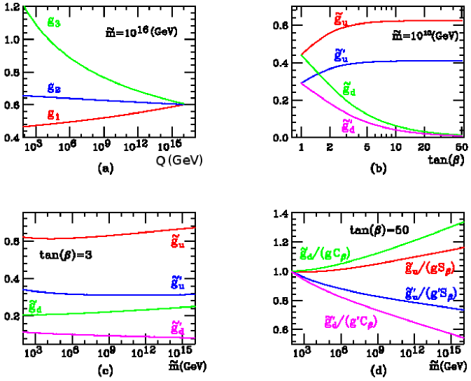
Figure 1: (a) Gauge coupling unification is preserved in Split-SUSY. (b) Split-Susy couplings dependence on $\tan\beta$. (c) Split-Susy couplings evaluated at weak scale as function of $\tilde{m}$. (d) Split-Susy couplings normalized with gauge couplings evaluated at weak scale, for different values of $\tilde{m}$.

The renormalization group equations for these and other couplings can be found in ref. Giudice:2004tc . For illustration we show in Fig. 1 some of their behaviour. In Fig 1(a) we have the running of the gauge coupling constants in Split Supersymmetry, which unify at the GUT scale as in the MSSM. In the second frame Fig. 1(b) we plot the Higgs-gaugino-higgsino couplings as a function of $\tan\beta$ for $\widetilde{m}=10^{16}$ GeV. If $\tan\beta=1$, neither the boundary condition nor the RGE differentiate between $\widetilde{g}_{u}$ and $\widetilde{g}_{d}$ or between $\widetilde{g}^{\prime}_{u}$ and $\widetilde{g}^{\prime}_{d}$. A sharp splitting appears when $\tan\beta$ increases. The down couplings become smaller than $0.1$ for $\tan\beta\>\raisebox{-2.15277pt}{$\stackrel{{\scriptstyle\textstyle>}}{{\sim}}$}\>10$, while the up couplings approach asymptotically a maximum as $\tan\beta$ increases. In Fig. 1(c) we plot the Higgs-gaugino-higgsino couplings as a function of the split supersymmetric scale $\widetilde{m}$. In Fig. 1(d) we plot the Higgs-gaugino-higgsino couplings normalized by the gauge couplings evaluated at the weak scale as a function of the scale $\widetilde{m}$. We choose the value $\tan\beta=50$, and observe deviations up to $\pm 20\%$. Of course, if the split supersymmetric scale is taken equal to the weak scale, there is no deviation.

Now we introduce the following notation,

$$\tan{\widetilde{\beta}}\ \equiv \ \displaystyle{\frac{\widetilde{g}_{u}}{\widetilde{g}_{d}}}\bigg{|}_{m_{W}}\simeq\tan{\beta}\left[1+\displaystyle{\frac{\cos{2\beta}}{64\pi^{2}}}\Big{(}7g^{2}(\widetilde{m})-3g^{\prime 2}(\widetilde{m})\Big{)}\ln\Big{(}\frac{\widetilde{m}}{m_{W}}\Big{)}\right]$$ (7)

$$\tan{\widetilde{\beta}^{\prime}}\ \equiv \ \displaystyle{\frac{\widetilde{g}_{u}^{\prime}}{\widetilde{g}_{d}^{\prime}}}\bigg{|}_{m_{W}}\simeq\tan{\beta}\left[1-\displaystyle{\frac{\cos{2\beta}}{64\pi^{2}}}\Big{(}9g^{2}(\widetilde{m})+3g^{\prime 2}(\widetilde{m})\Big{)}\ln\Big{(}\frac{\widetilde{m}}{m_{W}}\Big{)}\right]$$ (8)

where it is understood that $\beta$ is defined at the scale $\widetilde{m}$, while $\widetilde{\beta}$ and $\widetilde{\beta}^{\prime}$ are defined at the weak scale. The approximated expressions in eq. (8) is obtained from the corresponding RGE. These definitions together with,

$$\widetilde{g}^{2}\equiv\widetilde{g}_{u}^{2}(m_{W})+\widetilde{g}_{d}^{2}(m_{W}),\qquad\widetilde{g}^{\prime}{}^{2}\equiv\widetilde{g}^{\prime}_{u}{}^{2}(m_{W})+\widetilde{g}^{\prime}_{d}{}^{2}(m_{W}),$$ (9)

allow us to write the neutralino and chargino mass matrices in such a way it resembles those of the MSSM.

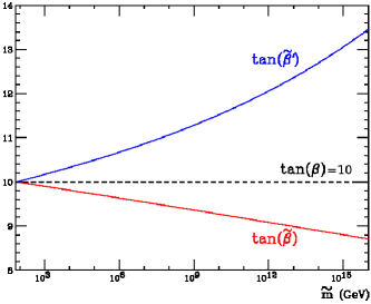
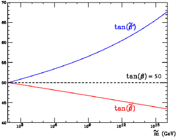
Figure 2: Dependence of $\tan{\widetilde{\beta}}$ and $\tan{\widetilde{\beta}^{\prime}}$ on the Split Supersymmetric scale, for different values of $\tan{\beta}$.

The mixing angles $\widetilde{\beta}$ and $\widetilde{\beta}^{\prime}$ are plotted in Fig. 2 as a function of $\widetilde{m}$ for $\tan\beta=10,50$. Of course, there is no difference between the three angles if $\widetilde{m}=M_{weak}$.

With this notation, the neutralino mass matrix in Split Supersymmetric models has the following form,

$${\bf M}_{\chi^{0}}^{SS}=\left[\begin{array}[]{cccc}M_{1}&0&-\frac{1}{2}\tilde{g}^{\prime}v\tilde{c}^{\prime}_{\beta}&\frac{1}{2}\tilde{g}^{\prime}v\tilde{s}^{\prime}_{\beta}\\ 0&M_{2}&\frac{1}{2}\tilde{g}v\tilde{c}_{\beta}&-\frac{1}{2}\tilde{g}v\tilde{s}_{\beta}\\ -\frac{1}{2}\tilde{g}^{\prime}v\tilde{c}^{\prime}_{\beta}&\frac{1}{2}\tilde{g}v\tilde{c}_{\beta}&0&-\mu\\ \frac{1}{2}\tilde{g}^{\prime}v\tilde{s}^{\prime}_{\beta}&-\frac{1}{2}\tilde{g}v\tilde{s}_{\beta}&-\mu&0\end{array}\right]$$ (10)

which is written in the usual basis $\psi^{0}=(\widetilde{B},\widetilde{W}^{3},\widetilde{H}_{d}^{0},\widetilde{H}_{u}^{0})$. We have used the notation $\tilde{c}^{\prime}_{\beta}\equiv\cos\tilde{\beta}^{\prime}$, $\tilde{c}_{\beta}\equiv\cos\tilde{\beta}$, $\tilde{s}^{\prime}_{\beta}\equiv\sin\tilde{\beta}^{\prime}$, $\tilde{s}_{\beta}\equiv\sin\tilde{\beta}$. This mass matrix is diagonalized by the matrix $N$, such that $N^{*}{\bf M}_{\chi^{0}}^{SS}N^{-1}=({\bf M}_{\chi^{0}}^{SS})_{diag}$, and the eigenvectors $\widetilde{\chi}_{i}^{0}=N_{ij}{\psi}_{j}^{0}$ are the neutralinos.

III Neutralino Decays in mSUGRA and Split Supersymmetry

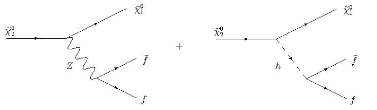
Figure 3: Tree-level three body decay diagrams in Split-SUSY for the second lightest neutralino.

In Split Supersymmetry the three body decay modes of the second lightest neutralino receive contributions from intermediate gauge and light Higgs bosons, with negligible contribution from sfermions and heavy Higgs boson. These graphs are in Fig. 3, where the major contribution is from the $Z$-boson exchange, since the fermions in the final states have a very small mass. We calculate these decay rates integrating over the phase space with numerical techniques. We compare our calculations for the case of a small SS scale $\widetilde{m}\sim 1$ TeV with results from the ISASUGRA code Paige:1998ux with $m_{0}\sim 1$ TeV. These are in agreement within small differences, the main of which is the distinctive running of Higgs-higgsino-gaugino couplings present is SS.

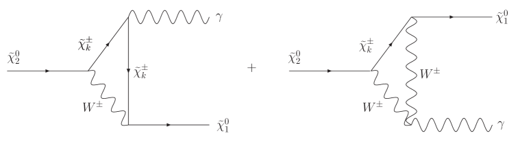
Figure 4: Diagrams for the second lightest neutralino radiative decay into a photon and the lightest neutralino in Split-SUSY.

Our main interest in this article is the radiative decay of the second lightest neutralino into the LSP and a photon. This one-loop generated decay can shed light into the properties of heavy particles present in the loop, charginos in the case of Split Supersymmetry. In addition, it is an experimentally interesting decay mode since includes only a hard photon plus missing energy. Contributing loops in SS are displayed in Fig. 4. The loops include both charginos and $W$ gauge bosons (charged Goldstone bosons are implicit). All other charged scalars which could contribute have a mass of the order of $\widetilde{m}$ and they are neglected. Of course, the effect of the heavy particles is felt via the RGE of the effective couplings below $\widetilde{m}$. We calculate the integral over internal momenta analytically using dilogarithms Haber:1988px .

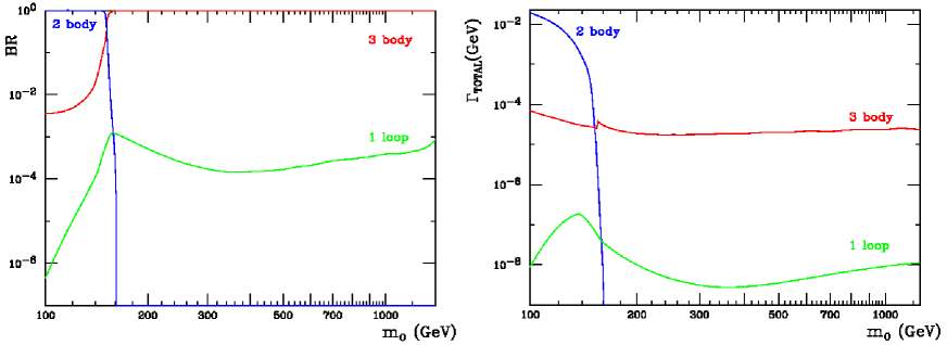
Figure 5: Branching ratio and decay width for the different neutralino decay modes, in mSUGRA as a function of $m_{0}$ and around the SPS1a benchmark point.

In Fig. 5 we show the behaviour of the three main decay modes of the second lightest neutralino in mSUGRA: the tree-level two-body decay $\chi^{0}_{2}\rightarrow\tilde{\ell}^{\pm}\ell^{\mp}$, the tree-level three-body decay $\chi^{0}_{2}\rightarrow\chi^{0}_{1}f\overline{f}$, and the one-loop two-body decay $\chi^{0}_{2}\rightarrow\chi^{0}_{1}\gamma$. We have Branching Ratios to the left and decay rates to the right, as a function of the universal scalar mass $m_{0}$. The tree-level modes are calculated with the code ISASUGRA, while the one-loop mode with our code. The other parameters are taken as in benchmark SPS1a snowmass , which is given in Table LABEL:tab:MSSMabc.

Table 1: Input parameters for SPS1a mSUGRA benchmark point.

Parameter	Value	Units
$m_{0}$	100	GeV
$M_{1/2}$	250	GeV
$A_{0}$	100	GeV
$\tan\beta$	10	-
${\mathrm{sign}}(\mu)$	+1	-

We can see that the one-loop decay rate $\Gamma(\chi^{0}_{2}\rightarrow\chi^{0}_{1}\gamma)$ has a maximum near $m_{0}=150$ GeV, decreasing for larger universal scalar mass. At values above $m_{0}=1$ TeV the mSUGRA result differs between 3-20% from our own SS result, calculated with values $\widetilde{m}\>\raisebox{-2.15277pt}{$\stackrel{{\scriptstyle\textstyle>}}{{\sim}}$}\>1$ TeV. Of course, it is expected that mSUGRA results approach the SS result for large $m_{0}$, since at large values of the universal scalar mass the triangular contributions from heavy scalar particles diminish. In SS the effect of these heavy particles appear through the RGE of the different couplings, but small differences remain between the two approaches because the running couplings include leading logarithm effects from all loops. We remind the reader that these RGE effects in SS do not spoil the unification of gauge coupling constants, as stressed in ref. Giudice:2004tc and illustrated in Fig. 1. The branching ratio $B(\chi^{0}_{2}\rightarrow\chi^{0}_{1}\gamma)$ remains between $10^{-3}$ and $10^{-4}$ for this mSUGRA scenario.

Table 2: Chargino and Neutralino masses for SPS1a.

Particle	Mass	Units
$\tilde{\chi}^{0}_{1}$	99	GeV
$\tilde{\chi}^{0}_{2}$	175	GeV
$\tilde{\chi}^{0}_{3}$	352	GeV
$\tilde{\chi}^{0}_{4}$	372	GeV
$\tilde{\chi}^{+}_{1}$	175	GeV
$\tilde{\chi}^{+}_{2}$	372	GeV

In Table LABEL:tab:chaneu we show the neutralino and chargino masses for $m_{0}=100$ GeV, with masses only slightly increasing (one or two GeV) for larger scalar mass, calculated using SUSPECT Djouadi:2002ze .

We compare in Fig. 5 the one-loop generated decay mode $\chi^{0}_{2}\rightarrow\chi^{0}_{1}\gamma$, with the tree-level decay modes. We define the tree-level two-body decay $\chi^{0}_{2}\rightarrow\tilde{\ell}^{\pm}\ell^{\mp}$ as the sum of the three leptonic decays $\chi^{0}_{2}\rightarrow\tilde{e}e,\tilde{\mu}\mu,\tilde{\tau}\tau$ which occurs for values $m_{0}\>\raisebox{-2.15277pt}{$\stackrel{{\scriptstyle\textstyle<}}{{\sim}}$}\>160$ GeV, where the sleptons have a mass smaller than $m_{\chi^{0}_{2}}$. In this region, this decay mode dominates with a branching ratio near unity. We also have the tree-level three-body decay $\chi^{0}_{2}\rightarrow\chi^{0}_{1}f\overline{f}$, where we sum over all possible fermions. Above $m_{0}\sim 160$ GeV the off-shell intermediate particles which contribute are the $Z$ gauge boson and the squarks or sleptons, depending whether the final state fermion is a quark or a lepton. In this region the $B(\chi^{0}_{2}\rightarrow\chi^{0}_{1}f\overline{f})$ is near unity. Below $m_{0}\sim 160$ GeV the contribution from the intermediate light on-shell sfermion is removed, and $B(\chi^{0}_{2}\rightarrow\chi^{0}_{1}f\overline{f})$ drops to a value between $10^{-3}$ and $10^{-2}$.

Table 3: Slepton and squark masses for SPS1a.

Particle	Mass	Units
$\tilde{e}_{R}$, $\tilde{\mu}_{R}$	145	GeV
$\tilde{e}_{L}$, $\tilde{\mu}_{L}$	204	GeV
$\tilde{\tau}_{1}$	136	GeV
$\tilde{\tau}_{2}$	208	GeV
$\tilde{t}_{1}$	375	GeV
$\tilde{b}_{1}$	491	GeV

In Table LABEL:tab:slepsqu we show the slepton and the lightest squark masses for the SPS1a scenario using SUSPECT. For larger $m_{0}$ these masses grow up sharply, with right selectron and smuon becoming on-shell if $m_{0}\>\raisebox{-2.15277pt}{$\stackrel{{\scriptstyle\textstyle<}}{{\sim}}$}\>150$ GeV and similarly for the lightest stau if $m_{0}\>\raisebox{-2.15277pt}{$\stackrel{{\scriptstyle\textstyle<}}{{\sim}}$}\>155$ GeV. Both thresholds are fused into one in Fig. 5 because of the low resolution used in the graph.

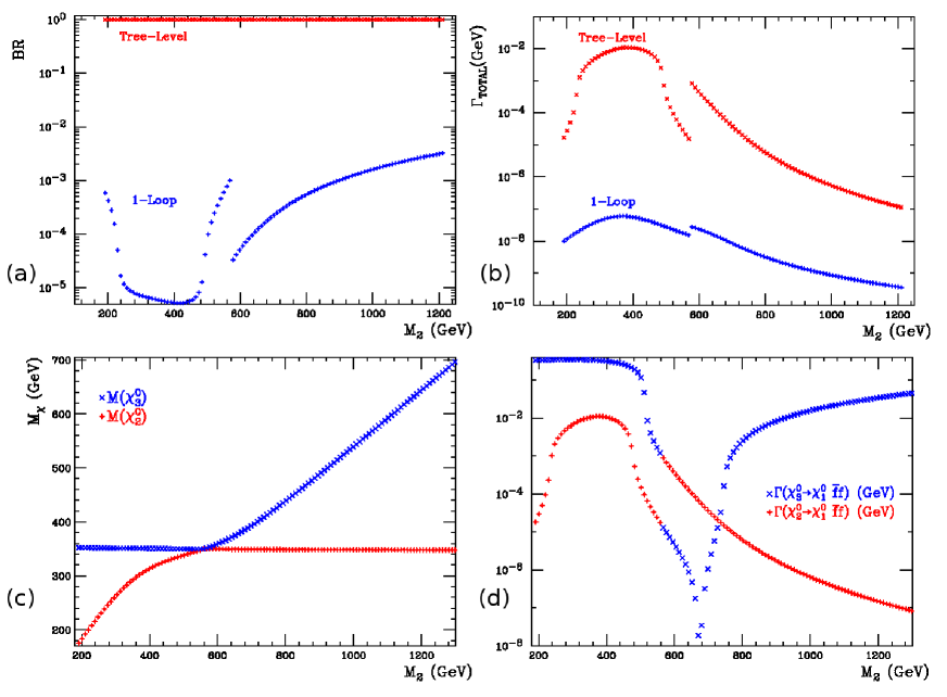
Figure 6: Branching ratio (a) and decay width (b) for $\tilde{\chi}^{0}_{2}$ decay modes in SS as a function of $M_{2}$. In (c) we see the mass eigenvalues crossing between the second and third neutralinos, which cause the discontinuous behaviour of the branching ratio and decay width (d).

In Fig. 6 we show the tree-level three-body decay $\chi^{0}_{2}\rightarrow\chi^{0}_{1}f\overline{f}$ and the one-loop two-body decay $\chi^{0}_{2}\rightarrow\chi^{0}_{1}\gamma$ in Split Supersymmetry, as a function of the wino mass $M_{2}$, both calculated with our own code.

Table 4: Input parameters for Split Supersymmetry benchmark point.

Parameter	Value	Units
$M_{1}$	102	GeV
$M_{2}$	192	GeV
$M_{3}$	587	GeV
$\mu$	357	GeV
$\tan\beta$	10	-

We choose as SS benchmark point the one given in Table LABEL:tab:M1M2mu, whose soft gaugino and higgsino mass values coincide with the low energy soft masses from SPS1a. When varying the wino mass $M_{2}$ in Fig. 6, we vary also the bino mass $M_{1}$ keeping constant the $M_{2}/M_{1}$ ratio as in our SS benchmark scenario. In frame (a) we have the branching ratios, where tree-level three-body decay dominates over the one-loop decay $\chi^{0}_{2}\rightarrow\chi^{0}_{1}\gamma$ with a BR near unity. Since we work in SS, the $\chi^{0}_{2}\rightarrow\chi^{0}_{1}f\overline{f}$ mode is mediated only by an intermediate $Z$ gauge boson. Similarly, the $\chi^{0}_{2}\rightarrow\chi^{0}_{1}\gamma$ decay is generated only by quantum corrections with $W$ gauge bosons and charginos inside the loop.

In frame (b) we plot the decay rates for these two modes. The discontinuity on both decay rates occur near $M_{2}\sim 560$ GeV and corresponds to an eigenvalue crossing. In frame (c) we see this eigenvalue crossing, with a $\tilde{\chi}^{0}_{3}$ higgsino type and $\tilde{\chi}^{0}_{2}$ gaugino type for $M_{2}\>\raisebox{-2.15277pt}{$\stackrel{{\scriptstyle\textstyle<}}{{\sim}}$}\>560$, while the opposite occurs for $M_{2}\>\raisebox{-2.15277pt}{$\stackrel{{\scriptstyle\textstyle>}}{{\sim}}$}\>560$. The effect of the crossing can be seen very clearly in frame (d) where we have the three-body decays for both neutralinos $\tilde{\chi}^{0}_{2}$ and $\tilde{\chi}^{0}_{3}$.

IV High Radiative Neutralino Decay Branching Ratio

In this chapter we analyze with more detail the radiative decay for the second lightest neutralino, and look for conditions for an enhanced $B(\chi^{0}_{2}\rightarrow\chi^{0}_{1}\gamma)$ in Split Supersymmetry.

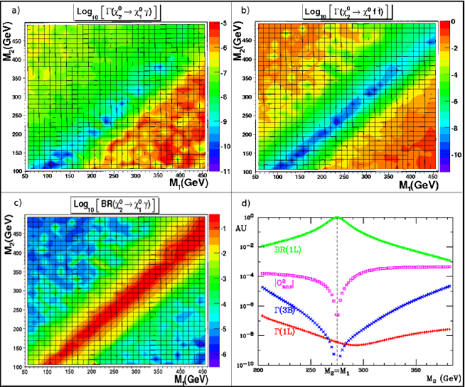
Figure 7: (a) Radiative decay width, (b) 3-Body decay width, and (c) Branching ratio for the radiative mode in $M_{1}$-$M_{2}$ plane in Split Supersymmetry. In (d) we have different curves as a function of $M_{2}$ showing the special behaviour at $M_{1}=M_{2}$.

In Fig. 7a we show with a color code the logarithmic values for the decay rate $\Gamma(\chi^{0}_{2}\rightarrow\chi^{0}_{1}\gamma)$ in the gaugino mass plane $M_{1}$-$M_{2}$, with $\Gamma$ measured in GeV. We show gaugino masses smaller than 500 GeV, and vary randomly the values for $\mu$ and $\tan\beta$. The largest values for the decay rate occur for $M_{1}>M_{2}$, reaching typically up to $10^{-5}$ GeV. In the opposite case, when $M_{1}<M_{2}$, the decay ratio varies typically between $10^{-7}$ and $10^{-8}$ GeV. There is a narrow fissure around $M_{1}\sim M_{2}$ where the decay rate drops to values between $10^{-10}$ and $10^{-11}$ GeV. The fissure is not exactly at the bisector but somewhat deviated to the $M_{1}>M_{2}$ side of the quadrant. In this fissure $\Delta m_{\chi}\equiv m_{\chi^{0}_{2}}-m_{\chi^{0}_{1}}$ is minimum, and the drop of the decay rate is a kinematical suppression.

In Fig. 7b we have a similar plot for the decay rate $\Gamma(\chi^{0}_{2}\rightarrow\chi^{0}_{1}f\overline{f})$, which is much larger than the previous case. This decay rate is more symmetrical with respect to the bisector, with decay rates reaching maximum values between $10^{-2}$ and 1 GeV, and a deep fissure at $M_{1}\sim M_{2}$ going all the way down to $10^{-11}$ GeV or smaller. The fissure is situated over the bisector, and it is due to a zero in the neutralino-neutralino-$Z$ coupling, i.e. a dynamical suppression.

The branching ratio for the radiative decay $B(\chi^{0}_{2}\rightarrow\chi^{0}_{1}\gamma)$ is shown in Fig. 7c. We see that the second lightest neutralino one-loop generated decay $\chi^{0}_{2}\rightarrow\chi^{0}_{1}\gamma$ can dominate in a wide zone near the bisector $M_{1}\sim M_{2}$. The reason for this possibility is that both decay rates decrease sharply in parallel fractures but slightly displaced. One of the fractures due to a zero in the $\chi^{0}\chi^{0}Z$ coupling (dynamical), and the other due to an eigenvalue degeneracy (kinematical). This is confirmed in Fig. 7d, where we show both decay rates, the radiative decay branching ratio, and the $\chi^{0}\chi^{0}Z$ coupling as a function of $M_{2}$, with constant values for $M_{1}=275$ GeV, $\mu=400$ GeV, $\tan\beta=10$, and $\widetilde{m}=10^{4}$ GeV. We see that the zero for $\Gamma(\chi^{0}_{2}\rightarrow\chi^{0}_{1}f\overline{f})$ coincides with the zero for $\chi^{0}\chi^{0}Z$ coupling at $M_{1}=M_{2}$, and that the minimum for $\Gamma(\chi^{0}_{2}\rightarrow\chi^{0}_{1}\gamma)$ coincides with the point where $m_{\chi^{0}_{2}}-m_{\chi^{0}_{1}}$ is minimum, at $M_{2}\>\raisebox{-2.15277pt}{$\stackrel{{\scriptstyle\textstyle>}}{{\sim}}$}\>M_{1}$.

In order to better understand the above result, it is instructive to see the neutralino mass matrix in the basis $[-i\widetilde{\gamma},-i\widetilde{Z},\widetilde{H}_{1},\widetilde{H}_{2}]$, where

$$\left[\begin{matrix}\widetilde{\gamma}\cr\widetilde{Z}\end{matrix}\right]=\left[\begin{matrix}c_{W}&s_{W}\cr-s_{W}&c_{W}\end{matrix}\right]\left[\begin{matrix}\widetilde{B}\cr\widetilde{W}\end{matrix}\right]\,,\qquad\qquad\left[\begin{matrix}\widetilde{H}_{1}\cr\widetilde{H}_{2}\end{matrix}\right]=\left[\begin{matrix}c_{\beta}&-s_{\beta}\cr s_{\beta}&c_{\beta}\end{matrix}\right]\left[\begin{matrix}\widetilde{H}_{d}\cr\widetilde{H}_{u}\end{matrix}\right]\,.$$ (11)

In this basis the mass matrix in eq. (10) looks as follows,

$${\bf M}_{\chi^{0}} = \left[\begin{array}[]{cc}{\bf M}_{\chi^{0}}^{gg}&{\bf M}_{\chi^{0}}^{gh}\\ {\bf M}_{\chi^{0}}^{hg}&{\bf M}_{\chi^{0}}^{hh}\end{array}\right]\hskip 11.38109pt$$ (14)

with ${\bf M}_{\chi^{0}}^{gh}=({\bf M}_{\chi^{0}}^{hg})^{T}$. The different submatrices are equal to,

$${\bf M}_{\chi^{0}}^{gg} = \left[\begin{array}[]{cc}M_{1}c^{2}_{W}+M_{2}s^{2}_{W}&(M_{2}-M_{1})s_{W}c_{W}\\ (M_{2}-M_{1})s_{W}c_{W}&M_{1}s^{2}_{W}+M_{2}c^{2}_{W}\end{array}\right]$$ (17)

$${\bf M}_{\chi^{0}}^{hh} = \left[\begin{array}[]{cc}\mu s_{2\beta}&-\mu c_{2\beta}\\ -\mu c_{2\beta}&-\mu s_{2\beta}\end{array}\right]$$ (20)

for the blocks in the diagonal, and

$${\bf M}_{\chi^{0}}^{gh}=\frac{v}{2}\left[\begin{array}[]{cc}c_{\beta}(\tilde{g}_{d}s_{W}-\tilde{g}^{\prime}_{d}c_{W})+s_{\beta}(\tilde{g}_{u}s_{W}-\tilde{g}^{\prime}_{u}c_{W})&s_{\beta}(\tilde{g}_{d}s_{W}-\tilde{g}^{\prime}_{d}c_{W})-c_{\beta}(\tilde{g}_{u}s_{W}-\tilde{g}^{\prime}_{u}c_{W})\\ c_{W}(c_{\beta}\tilde{g}_{d}+s_{\beta}\tilde{g}_{u})+s_{W}(c_{\beta}\tilde{g}^{\prime}_{d}+s_{\beta}\tilde{g}^{\prime}_{u})&c_{W}(s_{\beta}\tilde{g}_{d}-c_{\beta}\tilde{g}_{u})+s_{W}(s_{\beta}\tilde{g}^{\prime}_{d}-c_{\beta}\tilde{g}^{\prime}_{u})\end{array}\right]$$ (21)

for the off diagonal block. This neutralino mass matrix reduces to its analogous expression in the MSSM if we neglect the running from $\widetilde{m}$ and the weak scale:

$${\bf M}_{\chi^{0}}^{gh}\longrightarrow\frac{v}{2}\left[\begin{matrix}0&0\cr g/c_{W}&0\end{matrix}\right]\qquad{\mathrm{as}}\qquad\widetilde{m}\longrightarrow m_{weak}\,.$$ (22)

In the MSSM case, the direct mixing between photino and higgsinos vanishes, but a direct coupling between zino and one of the higgsinos remains. This implies that in general the lightest neutralino has a non vanishing component of higgsino, which in turn translates into a non vanishing $\chi^{0}\chi^{0}Z$ coupling. In this way, the photino will decouple from higgsinos in the region $M_{1}\sim M_{2}$, as seen from eq. (20), and the decay rate $\Gamma(\chi^{0}_{2}\rightarrow\chi^{0}_{1}f\overline{f})$ vanishes also, making the decay $\chi^{0}_{2}\rightarrow\chi^{0}_{1}\gamma$ the dominant one. In SS the mechanism is similar, but modified by RGE effects.

As we mentioned, in the dynamical suppression region where $M_{1}\sim M_{2}$ the decay mode $\Gamma(\chi^{0}_{2}\rightarrow\chi^{0}_{1}f\overline{f})$ is suppressed because the $Z$ coupling to the photino is absent, thus, when the LSP is nearly photino, the $Z\chi^{0}_{1}\chi^{0}_{2}$ coupling is nearly zero. In the MSSM this region does not exactly coincides with the kinematical suppression region where $m_{\chi^{0}_{1}}\sim m_{\chi^{0}_{2}}$ due to the remanent higgsino-gaugino mixing seen in eq. (22). In this case, phase space is small, and $\chi^{0}_{2}$ may be forced to decay into light mesons.

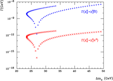
Figure 8: Decay rate for $\chi^{0}_{2}\longrightarrow\chi^{0}_{1}\pi^{0}$ in comparison to the decay rate for $\chi^{0}_{2}\longrightarrow\chi^{0}_{1}f\overline{f}$, as a function of the mass difference $\Delta m_{\chi}=m_{\chi_{2}}-m_{\chi_{1}}$.

The situation is similar in Split Supersymmetry where the difference lies in the fact that in SS RGE effects separate further the regions where $Z\chi^{0}_{1}\chi^{0}_{2}$ coupling and $\Delta m_{\chi}$ vanish, as indicated by the higgsino-gaugino mixing in eq. (21). In Fig. 8 we have plotted the decay rate $\Gamma(\chi^{0}_{2}\longrightarrow\chi^{0}_{1}f\overline{f})$ and the (included in the former) decay rate $\Gamma(\chi^{0}_{2}\longrightarrow\chi^{0}_{1}\pi^{0})$ as a function of $\Delta m_{\chi}$. The independent variable we are varying is $M_{2}$, exactly as in Fig. 7d. Both decay rates vanish at the point where the $Z\chi^{0}_{1}\chi^{0}_{2}$ coupling is null, but at that point $\Delta m_{\chi}$ is not zero. Indeed, in Fig. (8) we have $\Delta m_{\chi}=26.8$ GeV for $\widetilde{m}=10$ TeV, while RGE effects changes it to $\Delta m_{\chi}=29.2$ GeV for $\widetilde{m}=M_{GUT}$. Therefore, the photon in the decay $\chi^{0}_{2}\rightarrow\chi^{0}_{1}\gamma$ will have enough energy to be easily detected. Note that the two branches in each decay are defined by the sign of $M_{2}-M_{1}$.

As we discussed, in Split Supersymmetry the mechanism is analogous to the MSSM, but the details are modified by the Renormalization Group Equations effects. Indeed, the remaining higgsino component of the lightest neutralino in the case $M_{1}=M_{2}$ is controlled by the SS scale $\widetilde{m}$ via the RGE effects on the different couplings.

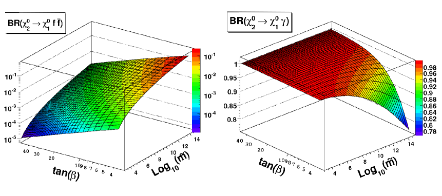
Figure 9: $\chi^{0}_{2}$ decay modes as a function of the Split Susy scale $\widetilde{m}$ and $tan\beta$ for the scenario where $M_{1}=M_{2}$.

This can be seen in Fig. 9 where we have the $\chi^{0}_{2}$ branching ratios dependence on $\tan\beta$ and the SS scale $\widetilde{m}$, with $\mu=400$ GeV and $M_{1}=M_{2}=275$ GeV. The dependence on $\tan\beta$ is relatively mild, as it is the dependence on $\widetilde{m}$. But in comparison to other observables, the dependence on the SS scale is very important, because in this scenario a measurement of the $\chi^{0}_{2}$ branching ratios could yield valuable information on the SS scale, otherwise difficult to extract from experiments. In the right frame we see that $B(\chi^{0}_{2}\rightarrow\chi^{0}_{1}\gamma)$ dominates over a large region, with a small decrease at small $\tan\beta$ and large $\widetilde{m}$. In the left frame we have $B(\chi^{0}_{2}\rightarrow\chi^{0}_{1}f\overline{f})$, with values that go from $10^{-5}$ up to $0.2$. Clearly, a measurement of the branching ratio can give valuable information on the split supersymmetric scale.

V Conclusion

We have calculated the decay rates and branching ratios of the second lightest neutralino in Split Supersymmetry, and concentrate in the radiative decay $\chi^{0}_{2}\rightarrow\chi^{0}_{1}\gamma$. We compared our results with mSUGRA, finding agreement when the scalar mass parameter is very large, $m_{0}\sim 1$ TeV, where $B(\chi^{0}_{2}\rightarrow\chi^{0}_{1}\gamma)\sim 10^{-3}$. Small differences remain due to RGE effects, which increase with larger split supersymmetric scale $\widetilde{m}$. For larger values of $m_{0}$ comparison is not possible since large squark masses in quantum corrections destabilize the EWSB in direct mSUGRA calculations.

In general models, the possibility that $m_{\chi^{0}_{2}}$ is not much different than the mass of the LSP is experimentally challenging. This is because the decay products that can be detected, photons in the case of $\chi^{0}_{2}\rightarrow\chi^{0}_{1}\gamma$ and fermions in the case of $\chi^{0}_{2}\rightarrow\chi^{0}_{1}f\overline{f}$, are soft and specialized analysis have to be done with the data. Nevertheless, in our model the radiative decay dominates in a region where $\Delta m_{\chi}$ is large enough to produce an energetic photon. We focus on the region $M_{1}\sim M_{2}$, where this possibility is realized and show that the decay $\chi^{0}_{2}\rightarrow\chi^{0}_{1}\gamma$ is dominant in a wide band around the bisector $M_{1}=M_{2}$. Furthermore, in this region a measurement of the branching ratios $B(\chi^{0}_{2}\rightarrow\chi^{0}_{1}\gamma)$ and $B(\chi^{0}_{2}\rightarrow\chi^{0}_{1}f\overline{f})$ can give information on the value of the split supersymmetric scale $\widetilde{m}$.

References

• (1) N. Arkani-Hamed and S. Dimopoulos, JHEP 0506, 073 (2005) [arXiv:hep-th/0405159].
• (2) G. F. Giudice and A. Romanino, “Split supersymmetry”, Nucl. Phys. B 699, 65 (2004) [Erratum-ibid. B 706, 65 (2005)] [arXiv:hep-ph/0406088].
• (3) F. Wang, W. Wang, F. q. Xu, J. M. Yang and H. Zhang, Eur. Phys. J.  C 51, 713 (2007) [arXiv:hep-ph/0612273]; S. K. Gupta, B. Mukhopadhyaya and S. K. Rai, Phys. Rev.  D 73, 075006 (2006) [arXiv:hep-ph/0510306]; M. A. Diaz and P. Fileviez Perez, J. Phys. G 31, 563 (2005) [arXiv:hep-ph/0412066]; K. Cheung and J. Song, Phys. Rev.  D 72, 055019 (2005) [arXiv:hep-ph/0507113].
• (4) G. Aad et al. [The ATLAS Collaboration], “Expected Performance of the ATLAS Experiment - Detector, Trigger and Physics,” arXiv:0901.0512 [hep-ex].
• (5) R. Adolphi et al. [CMS Collaboration], “The CMS experiment at the CERN LHC,” JINST 0803 (2008) S08004 [JINST 3 (2008) S08004].
• (6) G. Polesello, J. Phys. G 30 (2004) 1185.
• (7) H. E. Haber and D. Wyler, Nucl. Phys.  B 323, 267 (1989).
• (8) S. Ambrosanio and B. Mele, Phys. Rev.  D 55, 1399 (1997) [Erratum-ibid.  D 56, 3157 (1997)] [arXiv:hep-ph/9609212].
• (9) F. E. Paige, S. D. Protopopescu, H. Baer and X. Tata, “ISAJET 7.37: A Monte Carlo event generator for p p, anti-p p, and e+ e- reactions,” arXiv:hep-ph/9804321.
• (10) N. Ghodbane and H. U. Martyn, “Compilation of SUSY particle spectra from Snowmass 2001 benchmark models,” in Proc. of the APS/DPF/DPB Summer Study on the Future of Particle Physics (Snowmass 2001) ed. N. Graf, arXiv:hep-ph/0201233.
• (11) A. Djouadi, J. L. Kneur and G. Moultaka, “SuSpect: A Fortran code for the supersymmetric and Higgs particle spectrum in the MSSM,” Comput. Phys. Commun.  176, 426 (2007) [arXiv:hep-ph/0211331].