Self-organized global control of carbon emissions

Abstract

There is much disagreement concerning how best to control global carbon emissions. We explore quantitatively how different control schemes affect the collective emission dynamics of a population of emitting entities. We uncover a complex trade-off which arises between average emissions (affecting the global climate), peak pollution levels (affecting citizens’ everyday health), industrial efficiency (affecting the nation’s economy), frequency of institutional intervention (affecting governmental costs), common information (affecting trading behavior) and market volatility (affecting financial stability). Our findings predict that a self-organized free-market approach at the level of a sector, state, country or continent, can provide better control than a top-down regulated scheme in terms of market volatility and monthly pollution peaks.

A CO₂ emissions level of $\leq 500$ ppm SternReview would set the probability of a potentially catastrophic 5^∘C warming at 3$\%$SternReview . At a recent G8 summit, leaders agreed to ‘strongly consider’ at least halving global emissions by 2050bbc . However, there is still no national or international consensus on how these reductions can be systematically achieved and maintainedemissionstrading , nor is there any deep quantitative understanding of the trade-offs which could arise at the local and global level. Given the recent instabilities in global financial markets and apparent inevitability of human irrationalityGreenspan , it is also unclear whether a free-market approach can ever be trustedirrational .

Here we analyze a simple, yet realistic dynamical model of a competitive emissions market which allows us to investigate the simultaneous interplay between myriad competing real-world factors. Our model is a non-trivial generalization of the El Farol bar problemarthur which has attracted much attention among physicistschallet ; us ; neil . In addition to offering the physics community a novel generalization and application of the El Farol model, we believe that our work provides the first unified, quantitative discussion of the underlying trade-offs between average emissions, instantaneous peak pollution levels, market stability, efficiency of production, and common information. Our model predicts that a completely self-organized emissions market with collective competition and no top-down management, can offer distinct advantages over a managed system in terms of peak emission values. Although helpful with respect to the mean monthly emission, top-down monthly management can by contrast induce a far bigger volatility and hence aggravate the uncertainty in emissions.

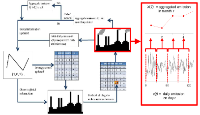
Figure 1: (Color) Schematic diagram of the carbon market model and the resulting daily time series $x(t)$ for day $t=1,2,\dots$, together with the aggregated monthly time-series $X(T)$ for month $T=1,2,\dots$.

Figure 1 shows a schematic describing our generic emissions scenario, comprising $N$ emitters (e.g. companies) who each decide whether to emit or not during a particular timestep $t$ (e.g. day). All companies are assumed to have the same emission capabilities (i.e., one unit of carbon each timestep). The system’s (e.g. national) safe emission level is $L$ over some period $\Delta t$ (e.g. month $\Delta t=30$), with successive periods (e.g. months) labelled $T=1,2,\dots$. Hence the average emission cap per timestep (e.g. day) is $\bar{L}=L/\Delta t$. Depending on the top-down management infrastructure of interest, the emitters could equally well be industries within a sector, companies within a state, states within a country, countries within a continent, or countries or continents within some global organization – likewise, the relevant timescales $t$ and $T$ need not be days and months respectively. From a governmental perspective, the ideal outcome would be that the total emission each month $X(T)$ is exactly equal to $L$ units of carbon pollutants: If $X(T)>L$ then too much carbon dioxide is emitted into the atmosphere, while $X(T)<L$ means that the nation has wasted some of its allowed production capacityemissionstrading . Companies are rewarded in some generic way (e.g. favorable public opinion, or a monetary compensation) for choosing to emit on low-pollution days ($x(t^{\prime})\leq\bar{L}$) or abstaining from emitting on high-pollution days ($x(t^{\prime})>\bar{L}$), and receive punishments otherwise. Each day’s outcome is represented in terms of its collective emission: 1 if $x(t^{\prime})\leq\bar{L}$ for a given $t^{\prime}$ and 0 if $x(t^{\prime})>\bar{L}$. Companies rely on common, publicly disclosed information when deciding whether or not to emit at a given timestep. We take this common information to be dominated by the previous $m$ days’ outcomes, a bit-string of length $m$ compromised by 0 or 1, but in principle it could include other information from government, public or other competitors. The fact that all participants have access to, and use, the same information, can generate correlations between their actions. A strategy is a specific prediction 0 or 1 (and hence action, emit or don’t emit) for each of the ${2^{m}}$ possible information bit-strings, hence there are $2^{2^{m}}$ strategies. Companies randomly select $s$ strategies from the strategy space with repetitions allowed during the assignment. Each company uses its best performing strategy at a given timestep, with an individual strategy’s score updated by $+1$ ($-1$) at a given timestep, if it would have made the correct (incorrect) decision. The correct decisions are emitting (not emitting) when the cap is not exceeded (exceeded), and vice versa for incorrect decisions. Tied best-performing strategies are broken by random choices. Our setup therefore incorporates the generic complex system features of Arthur’s El Farol problem and Challet and Zhang’s binary versionarthur ; challet ; us ; neil . Most importantly, companies do not communicate directly among themselves, nor do they need to know the number of competitors around, nor are they managed by some governmental entity. Instead, by competing to emit, they interact through the common information that their collective actions create. There is recent independent evidence that groups of human do indeed employ such general decision-based mechanisms as in Fig. 1PNASmg . More generally, our model mimics a simple cap-and-trade scenario in which emitters who decide to emit on a given day immediately purchase a permit to do so. The less emitters per day, the lower the demand for permits, and hence the lower that day’s permit price, and vice versa. Hence the time-series of emissions $x(t)$ mimics the time-series of permit prices.

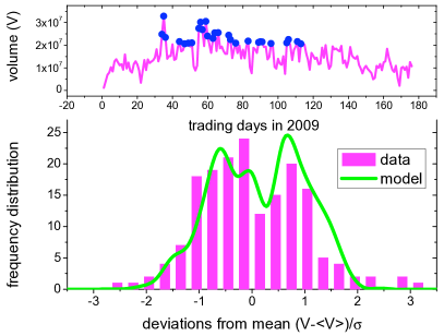
Figure 2: (Color) The upper panel is the daily time series of the first $176$ trading days’ total volume in $2009$ from ECX EUA futures contract, in tonnes of CO₂ (EU allowances). The lower panel shows the empirical frequency distribution of $(V-\langle V\rangle)/\sigma)$, as compared to our model $m=4$, averaged over $100$ runs. Our model is a good representation of the empirical data, but has the added advantage that it eliminates the extreme peaks observed in the EU market (indicated by circles in the top panel). This suggests that our unmanaged free market mechanism would provide tighter control than the existing EU market.

Figure 2 shows that this simple model is capable of reproducing the highly irregular, non-Gaussian distribution of the 2009 EU carbon market to date. The model parameters and their values have a direct and reasonable interpretation: $N=100$ suggests that the actions of approximately one hundred entities (e.g. large companies) is moving the market in 2009, and hence visibly impacting the overall emissions; $m=4$ suggests that just less than one week of prior outcomes is considered relevant for making a decision; $s=6$ suggests that individual entities are using approximately six strategies to make a decision about whether to buy a permit and hence emit. Choosing to emit is equivalent to buying a permit and using it on that day – if less people apply on a given day, the permit price is low which means that the time-series of the number of emitters and the price mimic each other. Hence as a surrogate of the actual daily emissions, we have taken the daily carbon price to represent the daily demand for permission to emit, and hence the resulting volume of emissions. The quantity displayed, $(V-\langle V\rangle)/\sigma$, is independent of the number of participants $N$, for large $N$. We note that our model shows a smaller occurrence of extreme events than the empirical data, suggesting that our competitive, self-organized setup might provide better control of large fluctuations than the present EU scheme which is operating. If the distribution were more Gaussian-like as in regular financial markets, this would suggest that the market should contain many noisy speculators – however, the multi-modal form in Fig. 2 implies that this is not the case.

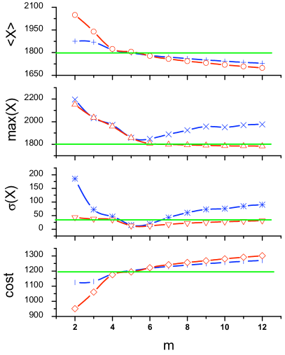
Figure 3: (Color) Monthly emissions for our model, for $N=100$, $s=6$. Top to bottom: the mean monthly emission $\langle X\rangle$, the maximum (i.e. peak) monthly emission, the monthly volatility $\sigma(X)$, and the governmental cost of compensation to companies for not emitting. Red: unmanaged system. Blue: managed system. Green: random result for learning $p=\bar{L}/N$.

Figure 3 compares the predictions of our model for monthly emissions between an unmanaged (red curve) and managed (blue curve) system, as a function of the amount of common information about previous outcomes (i.e. $m$). The average daily emissions cap is $\bar{L}=60$. In the managed system, at the end of month $T$, the government will reduce or increase the emissions capacity ${L}(T+1)$ for month $T+1$ by the amount that the aggregated emissions $X(T)$ was above or below ${L}(T)$. In the unmanaged system, there is no such external control and hence ${L}$ is constant. The overall system performance can be assessed through the time-series for monthly emissions $X(T)$ (Fig. 1): In particular (top to bottom in Fig. 3) the mean $\langle X\rangle$, the maximum ${\rm max}(X)$ (where ${\rm max}(X)$ is the largest monthly emission value during the time-window of the numerical simulation) over some fixed period (e.g. a year), and the standard deviation (i.e. volatility $\sigma(X)$) about the mean. An interesting comparison system is obtained by considering the ‘random’ case of an unmanaged system in which companies decide to emit by tossing a coin each day. In the absence of any learning (i.e. the system is non-adaptive) every decision is an independent coin toss and hence the a priori probability to emit would be $p=0.5$. However if the entities are gradually able to learn from the feedback of the previous experience and adapt to the ideal ratio $\bar{L}/N$ (at least, at the collective level) then $p=\bar{L}/N$ yielding the green curves shown in Fig. 3.

The mean monthly emission $\langle X\rangle$ decreases monotonically as $m$ increases for both systems. The monthly control exerted in the managed system pulls the value closer to the capacity limit of $1800$ than for the unmanaged system. However, this improved performance due to top-down management is accompanied by a significantly higher volatility for $m>6$ as well as a significantly higher peak pollution level. Indeed, the managed system does worse than both the unmanaged system and the random system with learning. This is because the month-by-month adjustment to $\bar{L}$ induces a delayed oscillatory effect which in turn generates significant volatility. A transition occurs around $m\sim 4$ where all the curves seem to cross the green (i.e. random learning) curve. This $m$ value coincides with the system’s dynamical de Bruijn path (which has duration $2.2^{m}$ m4 ) becoming equal to the finite duration of the emission interval (i.e. 30 days, hence $2.2^{m}\sim 30$ which yields $m\sim 4$). This precedes a minimum in the volatility around $m\sim 5$ for both managed and unmanaged systems, which is smaller than for random learning. As for the El Farol problemarthur ; challet ; us ; neil , this unintentional collective cooperation emerges as a result of cancellation between the actions of crowds of emitters using one strategy, and anticrowds using the exact opposite strategy. The cost result (bottom panel) reflects a simple one-unit payout given to any company not emitting on a given day. The choice of emitting or not-emitting becomes essentially cost-neutral to a given company – however for public relations reasons, and because they want to stay active in business, each company still continues to compete. A higher $\langle X\rangle$ hence incurs a lower cost.

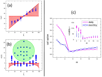
Figure 4: (Color) Daily emissions for our model with $m$ varying from 2 to 12 ($s=6$). Red shaded region is the analytically obtained zone of learning (see text). (a) Mean emission. Horizontal boundary line corresponds to no learning, diagonal boundary line (slope of unity) is for learning. (b) Volatility. Horizontal boundary line corresponds to no learning, convex curve is for learning. Green shaded circle shows low $m$, high volatility region due to crowding in strategy space. (c) European call option prices for different measurements of volatility according to the standard derivative pricing theory (i.e. Black-Scholes equation). Risk-free interest rate $r=0$, current value $x$ is set to the individual mean divided by 100, and strike price $X_{s}$ equals $\bar{L}/100$. The volatility $\sigma$ is scaled by $1/\sqrt{100}$. The time is one day before expiration. Blue curve uses the results from monthly measurement, while purple one is from daily measurement. The insert shows the anomalous scaling of volatility of emissions, from daily to monthly scales. There are $64$ runs for each $m$. The purple crosses are the standard deviation calculated by taking the daily volatility and multiplying by $\sqrt{30}$, which would be exactly equal to the monthly volatility if the time-series followed a random walk.

Figure 4 shows the model’s daily emission (Fig. 4(a), crosses) and volatility (Fig. 4(b), crosses) as a function of the daily emissions cap $\bar{L}$. The red shaded area in Figs. 4(a) and (b) is the ‘learning zone’ bounded by the two analytically obtained limits of no learning ($p=0.5$, the probability that a company is going to emit at a timestep, horizontal red line) and learning ($p=\bar{L}/N$, red diagonal line in Fig. 4(a) and convex curve in Fig. 4(b)). The standard deviation for daily emissions in the random case, is given analytically by the usual binomial form, i.e. $[Np(1-p)]^{\frac{1}{2}}$. Using the lower bound value $p=\bar{L}/N$ yields the convex curve $[\bar{L}(1-\bar{L}/N)]^{\frac{1}{2}}$, while using the upper bound value $p=0.5$ yields the horizontal line $0.5N^{\frac{1}{2}}=5$. The model’s mean emission values (crosses) lie within the shaded area in Fig. 4(a) but are closest to the limit $p=\bar{L}/N$, thereby demonstrating that the unmanaged, self-organized market collectively learns. For intermediate $\bar{L}$ values (Fig. 4(b)) the corresponding volatility tends to be smaller than the random value, however it moves above it for very large or small $\bar{L}$. For small $m$ values, which corresponds to the crowded regime of the strategy space, numerical runs can show significantly large volatilities (green circle).

Figure 4(c) explores the implications of our results for the derivative emissions markets. If emission markets follow the path of the mature non-emission financial markets, it is likely that such derivatives (e.g. options) markets will become as large, or even larger, than the primary emissions market itselfneil . In this respect, our findings serve as a warning of the dangers of simply applying standard financial theory for such derivative instrumentsneil . Standard option pricing theory uses the volatility over a given time increment as the input to the Black-Scholes pricing formulaprice . This assumes that the market approximates to a random walk and hence that the monthly volatility over $\Delta t$ timesteps is simply the volatility over one timestep multiplied by $\sqrt{\Delta t}$. Figure 4(c) shows not only that this is incorrect (see inset), but also that the discrepancy depends on the amount of common information $m$ – and that as a consequence, the price of a call option (Fig. 4(c)) can be mispriced according to whether daily or monthly volatility estimates are used. This opens up an intriguing but dangerous situation in the event of any abnormal periods in the market: Following some external news event (e.g. collapse of an oil company), it may happen that the number of previous days’ outcomes that are thought relevant, becomes very small (i.e. $m\rightarrow 0$). As shown, the corresponding mispricing then becomes huge, leading to possible financial instabilities.

Despite recent skepticism surrounding the stability of free markets, our analysis predicts that an unmanaged carbon emissions market can provide significant advantages over a managed one. For a given sector, state, country or continent, our model helps identify the appropriate degree of governmental management such that annual global emissions targets are achieved, while simultaneously allowing for individual choice regarding the trade-off between local social issues as listed in the abstract. Finally, we have checked that our main conclusions are reasonably robust to different sets of parameter values.

References

- (1) N. Stern, The Economics of Climate Change: The Stern Review. (Cambridge Univ. Press, Cambridge, 2007); A Blueprint for a Safer Planet. (Random House, London, 2009), pp. 39; A.D. Ellerman, et al. Markets for Clean Air: The U.S. Acid Rain Program. (Cambridge Univ. Press, Cambridge, 2000).
- (2) See news.bbc.co.uk/1/hi/world/europe/6732787.stm
- (3) Emission Trading: Environmental Policy’s New Approach, Eds. R.F. Kosobud, D.L. Schreder, and H.M. Biggs (John Wiley Sons, Inc., New York, 2000); Voluntary Carbon Markets: An International Business Guide to What They Are and How They Work Eds. R. Bayon, A. Hawn, and K. Hamilton (Earthscan Publications Ltd., London, 2009); Emission Trading: institutional Design, Decision Making and Corporate Strategies, Eds. R. Antes, B. Hansjurgens, and P. Letmathe (Springer, New York, 2008).
- (4) See news.bbc.co.uk/2/hi/business/8244600.stm
- (5) J. O’Brien, Engineering a Financial Bloodbath. (World Scientific, Singapore, 2009).
- (6) W.B. Arthur, Amer. Econ. Assoc. Papers. Proc. 84, 405 (1994); Science 284, pp. 107-109 (1999).
- (7) D. Challet, and Y.C. Zhang, Physica A 246, 407 (1997); D. Challet, M. Marsili, and Y.C. Zhang, Minority Games. (Oxford Univ. Press, 2005); A.C.C. Collen, The mathematical theory of Minority Games. (Oxford University Press, 2005); T.Galla, D. Sherrington, J. Stat. Mech. P 10009 (2005); D. Sherrington, E. Moro, and J.P. Garrahan, Physica A 311, 527 (2002); T. Galla, and A. De Martino, J. Phys. A: Math. and Theor. 41 324003 (2008).
- (8) N.F. Johnson, et al. Physica A 258, 230 (1998).
- (9) N.F. Johnson, P. Jefferies, and P.M. Hui, Financial Market Complexity. (Oxford Univ. Press, 2003).
- (10) W. Wang, Y. Chen, and J. Huang, Proc. Natl. Acad. Sciences. U.S.A. 106, 8423 (2009).
- (11) P. Jefferies, M.L. Hart, and N.F. Johnson, Phys. Rev. E 65, 016105 (2001).
- (12) Price of the European call option, using Black-Scholes equation, isneil : , where , , , where is the volatility.