Classical Strongly Coupled QGP:
VII. Energy Loss

Abstract

We use linear response analysis and the fluctuation-dissipation theorem to derive the energy loss of a heavy quark in the SU(2) classical Coulomb plasma in terms of the $l=1$ monopole and non-static structure factor. The result is valid for all Coulomb couplings $\Gamma=V/K$, the ratio of the mean potential to kinetic energy. We use the Liouville equation in the collisionless limit to assess the SU(2) non-static structure factor. We find the energy loss to be strongly dependent on $\Gamma$. In the liquid phase with $\Gamma\approx 4$, the energy loss is mostly metallic and soundless with neither a Cerenkov nor a Mach cone. Our analytical results compare favorably with the SU(2) molecular dynamics simulations at large momentum and for heavy quark masses.

I Introduction

Parton energy loss at RHIC is widely viewed as a way to probe the properties of the medium created during the first few fm/c of the collision. The medium is suspected to be a strongly coupled liquid shuryak2 with near perfect fluidity and strong energy loss.

There have been a number of calculations involving parton collisional thoma&gyulassy ; braaten&thoma ; braaten&thoma2 ; djordjevic and radiative djordjevic&heinz ; djordjevic&heinz2 energy loss at RHIC with the chief consequence of jet quenching dumitruetal . The measured jet quenching at RHIC exceeds most current theoretical predictions, most of which are based on a weakly coupled quark-gluon plasma (wQGP).

The QCD matter probed numerically using lattice simulations and at RHIC using heavy ion collisions, is likely to be dominated by temperatures in the few $T_{c}$ range making it de facto non-perturbative. Non-perturbative methods are therefore welcome for analyzing the QCD matter conditions in this temperature range. An example being the holographic method as a tool for jet quenching analysis sin&zahed ; liuetal .

In this letter, we follow the approach suggested in gelmanetal ; gelmanetal2 ; cho&zahed ; cho&zahed2 to model the strongly coupled quark and gluon plasma, by classical colored constituents interacting via strong Coulomb interactions. This model has been initially analyzed using Molecular Dynamics (MD) simulations mostly for the SU(2) version with species of constituents (gluons). The MD results reveal a strongly coupled liquid at $\Gamma\approx 4$ the ratio of the mean kinetic to Coulomb energy (modulo statistical fluctuations). The fractional energy loss is also found to be considerably larger than most leading order QCD estimates.

Here, we will provide the analytical framework to analyze the MD simulation results for partonic energy loss in the cQGP. In section 2, we outline a formal derivation of the energy loss in the cQGP for arbitrary values of $\Gamma$. In section 3, we use linear response theory and the fluctuation-dissipation theorem to tie the energy loss to the non-static colored structure factor. In section 4, we derive explicitly the non-static structure factor using the Liouville equation. Some useful aspects of the plasmon excitations in the cQGP are discussed in section 5. In section 6, we analyze the energy loss for both charm and bottom for $\Gamma=$2,3 and 4 in the liquid phase and compare them to the recent SU(2) MD simulations dusling&zahed . In section 7, we discuss the relevance of our results to RHIC and holographic QCD.

II Energy Loss

Consider an SU(2) colored particle of charge $q^{a}$ travelling with velocity $v$ in the strongly coupled colored plasma gelmanetal . The equation of motion of this extra particle in phase space follows from the Poisson bracket

$$\frac{d\boldsymbol{p}_{i}}{dt}=-\{H,\boldsymbol{p}_{i}\}=q^{a}\cdot\boldsymbol{E}_{in}^{a}$$ (II.1)

with the longitudinal colored electric field

$$\boldsymbol{E}_{in}^{a}=-\boldsymbol{\nabla}\sum_{i}\frac{Q^{a}_{i}(t)}{|\boldsymbol{r}-\boldsymbol{r}_{i}(t)|}=-\boldsymbol{\nabla}_{i}\Phi^{a}_{in}(t,\boldsymbol{r})$$ (II.2)

We note that in gelmanetal the SU(2) plasma is considered mostly electric with massive constituents $m\beta\approx 3$. As a result the transverse electric contribution is absent in (II.2). Also, (II.1) does not involve the magnetic part of the Lorentz force for the same reasons. The latter is irrelevant for the energy loss per travel length $\boldsymbol{r}=\boldsymbol{v}t$

$$\frac{dK}{dr}=\boldsymbol{v}q^{a}\boldsymbol{E}_{in}^{a}(t,\boldsymbol{r}=\boldsymbol{v}t)$$ (II.3)

even in the ultrarelativistic case since the magnetic force does not perform work.

The induced colored Coulomb potential $\Phi_{ind}$ follows from the total colored potential $\Phi_{\rm tot}$ through

$$\Phi^{a}_{tot}(\omega,\boldsymbol{k})=\Phi^{a}_{ind}(\omega,\boldsymbol{k})+\Phi^{a}_{ex}(\omega,\boldsymbol{k})=\frac{\Phi^{a}_{ex}(\omega,\boldsymbol{k})}{\epsilon_{L}(\omega,\boldsymbol{k})}$$ (II.4)

The last relation defines the longitudinal dielectric constant with $\boldsymbol{\Phi}_{ex}(\omega,\boldsymbol{k})=\frac{4\pi}{k^{2}}2\pi\boldsymbol{q}\delta(\omega-\boldsymbol{k}\cdot\boldsymbol{v})$, the colored potential caused by the extra particle in the probe approximation (ignoring back reaction). Thus

$$\Phi^{a}_{ind}(t,\boldsymbol{r})=q^{a}\int\frac{d\boldsymbol{k}}{(2\pi)^{3}}\left(\frac{1}{\epsilon_{L}(k\cdot v,\boldsymbol{k})}-1\right)\,\frac{4\pi}{k^{2}}e^{i\boldsymbol{k}\cdot\boldsymbol{r}-i\boldsymbol{k}\cdot\boldsymbol{v}t}$$ (II.5)

Using (II.2) and (II.3) we have for the energy loss of a fast moving probe SU(2) charge

$$-\frac{dK}{dr}=-\frac{\boldsymbol{q}^{2}}{\pi v^{2}}\int\frac{dk}{k}\int_{-kv}^{kv}\omega d\omega\Im\left(\frac{1}{\epsilon_{L}(\omega+i0,\boldsymbol{k})}\right)$$ (II.6)

after using the analytical property of $\epsilon_{L}(z,k)=\epsilon_{L}(-z^{*},-k)$ which follows from the causal character of the longitudinal dielectric function as detailed below. (II.6) is identical in form to the one derived for the Abelian one component colored Coulomb plasma in ichimaru , to the exception of the SU(2) classical Casimir $\boldsymbol{q}^{2}$ in (II.6). It is different in content through the longitudinal dielectric constant $\epsilon_{L}$ which now should be derived for a colored SU(2) Coulomb plasma. Our derivation is fully non-Abelian in the probe approximation.

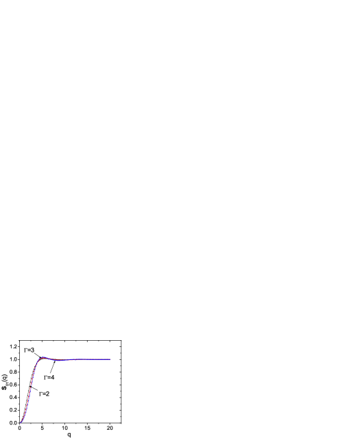
Figure 1: Static structure factors for $\Gamma=2,3,4$

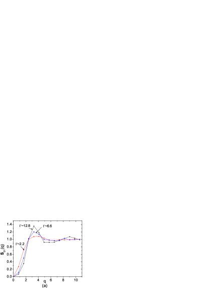
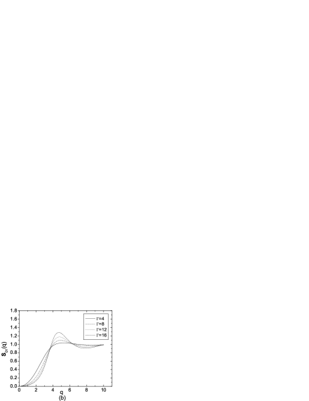
Figure 2: ${\bf S}_{01}(q)$: molecular dynamics simulation (a) and analytic (b). See text.

Below we show that for the SU(2) colored Coulomb plasma at strong Coulomb coupling, (II.6) reads

$$-\frac{dK}{dr}=-\frac{\boldsymbol{q}^{2}}{\pi v^{2}}\int\,\frac{dk}{k^{3}}\,\frac{k_{D}^{2}\,{\bf S}_{01}(k)}{1-{\bf S}_{01}(k)}\int_{-kv}^{+kv}\,d\omega\,\omega\,\Im\left(\frac{1}{\epsilon_{1}(\omega+i0,\boldsymbol{k})}\right)$$ (II.7)

with $k_{D}^{2}$ the SU(2) Debye wave number squared. Here

$$\epsilon_{1}(z,\boldsymbol{k})=1-n\,{\bf c}_{D1}(\boldsymbol{k})\,{\bf W}(z/\omega_{T})$$ (II.8)

with the thermal frequency $\omega_{T}=v_{T}k$ and velocity $v_{T}=\sqrt{T/m}$ and

$${\bf W}(z/\omega_{T})=\frac{1}{\sqrt{2\pi}}\int_{-\infty}^{+\infty}dt\,\frac{t}{t-z/\omega_{T}}\,{e^{-t^{2}/2}}$$ (II.9)

The l=1 static structure factor ${\bf S}_{01}$ cho&zahed3

$${\bf S}_{01}(k)=\left<\left|\sum^{N}_{j=1}e^{i\boldsymbol{k}\cdot\boldsymbol{r}_{j}}\,Q_{j}^{a}\right|^{2}\right>$$ (II.10)

satisfies the generalized Ornstein-Zernicke equation

$${\bf S}_{01}(k)=\frac{1}{1-n{\bf c}_{D1}(k)}$$ (II.11)

in the colored Coulomb plasma with 1 species density $n=N/V$. In Fig. 1 we show analytical results for (II.10) around the liquid point cho&zahed3 . In Fig. 2a we show the behavior of (II.10) using SU(2) molecular dynamics simulations with the dimensionless wavenumber $q=k\,a_{WS}$ where $a_{WS}$ is the Wigner-Seitz radius through $1/n=4\pi\,a_{WS}^{3}/3$. In Fig. 2b we show the analytical results for the same range of $\Gamma$ in cho&zahed3 .

The $l=1$ contribution $\epsilon_{1}$ plays the role of a generalized longitudinal dielectric constant in the SU(2) Coulomb plasma. Indeed, for weak Coulomb coupling $\Gamma\ll 1$, $-n{\bf c}_{D1}\approx k_{D}^{2}/k^{2}$ so that ${\bf S}_{01}\approx k^{2}/(k^{2}+k_{D}^{2})$. The energy loss (II.7) reduces to (II.6) with $\epsilon_{L}\rightarrow\epsilon_{1}$. At weak coupling $\epsilon_{1}$ in (II.8) is the standard Vlasov dielectric function in ichimaru . The only difference is in the SU(2) Debye wave number.

III Linear Response

To construc the longitudinal dielectric constant for the SU(2) Coulomb plasma we will make use of the Liouville kinetic equations for the time dependent structure factors derived in cho&zahed3 . For that we recall that in linear response, the induced color charge density $\rho_{ind}^{a}=\nabla\cdot E_{ind}^{a}/4\pi$ ties with the external potential $\Phi_{ext}^{b}$ through the retarded correlator

$$\rho_{ind}^{a}(t,\boldsymbol{r})=i\int\,dt^{\prime}\,d\boldsymbol{r}^{\prime}\,\left<{\bf R}\left({\bf J}_{0}^{a}(t,\boldsymbol{r}){\bf J}_{0}^{b}(t^{\prime},\boldsymbol{r}^{\prime})\right)\right>\,{\Phi}_{ext}^{b}(t^{\prime},\boldsymbol{r}^{\prime})$$ (III.1)

where ${\bf J}_{0}^{a}$ are the pertinent color charge densities. In Fourier space we have

$$\Phi_{ind}^{a}=-\frac{4\pi}{k^{2}}\,\Delta^{ab}_{R}(\omega,\boldsymbol{k})\,\Phi_{ext}^{b}$$ (III.2)

with

$$\Delta_{R}^{ab}(\omega,\boldsymbol{k})=-i\int\,e^{-i\omega t+i\boldsymbol{k}\cdot\boldsymbol{r}}\,\left<{\bf R}\left({\bf J}_{0}^{a}(t,\boldsymbol{r}){\bf J}_{0}^{b}(t^{\prime},\boldsymbol{r}^{\prime})\right)\right>$$ (III.3)

A comparison of (III.2) with (II.4) yields

$$\left(\frac{1}{\epsilon_{L}(\omega,\boldsymbol{k})}-1\right)\,\delta^{ab}=-\frac{4\pi}{k^{2}}\,\Delta_{R}^{ab}(\omega,\boldsymbol{k})$$ (III.4)

which defines the longitudinal dielectric constant.

The retarded correlator (III.3) is in general a quantum object, we now show how to extract it from the correlations in the classical and strongly coupled SU(2) colored Coulomb plasma. For that, we note that the colored charge density in the SU(2) phase space is

$${\bf J}_{0}^{a}(t,\boldsymbol{r})=\int\,dQ\,d\boldsymbol{p}\,Q^{a}\delta f(t,\boldsymbol{r},\boldsymbol{p},\boldsymbol{Q})$$ (III.5)

and that the SU(2) charge-charge correlator is

$$\left<{\bf J}_{0}^{a}(t,\boldsymbol{r}){\bf J}_{0}^{b}(t^{\prime},\boldsymbol{r}^{\prime})\right>=\frac{1}{3}\delta^{ab}\int\,dQ\,dQ^{\prime}\,d\boldsymbol{p}\,d\boldsymbol{p}^{\prime}\,\boldsymbol{Q}\cdot\boldsymbol{Q}^{\prime}\,{\bf S}(t-t^{\prime},\boldsymbol{r}-\boldsymbol{r}^{\prime},\boldsymbol{p}\boldsymbol{p}^{\prime},\boldsymbol{Q}\cdot\boldsymbol{Q}^{\prime})$$ (III.6)

where global time, space and color invariances were used thanks to the statistical averaging. The time dependent structure factor ${\bf S}=\langle\delta f\delta f\rangle$ was defined in cho&zahed3 . Using the color Legendre transform of ${\bf S}$ yields

$$\left<{\bf J}_{0}^{a}(t,\boldsymbol{r}){\bf J}_{0}^{b}(t^{\prime},\boldsymbol{r}^{\prime})\right>=\delta^{ab}\int\,d\boldsymbol{p}\,d\boldsymbol{p}^{\prime}\,{\bf S}_{1}(t-t^{\prime},\boldsymbol{r}-\boldsymbol{r}^{\prime},\boldsymbol{p}\boldsymbol{p}^{\prime})$$ (III.7)

Only the $l=1$ partial wave in the Legendre transform of the color part of ${\bf S}$ contributes to the SU(2) charge-charge correlation function.

The fluctuation-dissipation theorem in the classical limit ties the retarded correlator $\Delta_{R}$ in (III.3) to the Fourier transform of the classical phase space fluctuations (III.7) as

$$\Im\Delta^{ab}_{R}(\omega,\boldsymbol{k})=\delta^{ab}\frac{n\omega}{2T}\,{\bf S}_{1}(\omega,\boldsymbol{k})\equiv-\delta^{ab}\frac{n\omega}{T}\,\Im{\bf S}_{1}(z,\boldsymbol{k})$$ (III.8)

The last relation follows from ${\bf S}_{1}(\omega,\boldsymbol{k})=-2\,{\rm Im}\,{\bf S}_{1}(\omega,\boldsymbol{k})$ between the Laplace transform and Fourier transform of ${\bf S}_{1}$ with $z=\omega+i0$.

IV Non-Static Structure Factor

We have shown in cho&zahed4 that the l-color partial wave of the Laplace transform of ${\bf S}_{l}$ obeys the Liouville equation

$$z{\bf S}_{l}(z\boldsymbol{k};\boldsymbol{p}\boldsymbol{p}^{\prime})-\int d\boldsymbol{p}_{1}\Sigma_{l}(z\boldsymbol{k};\boldsymbol{p}\boldsymbol{p}_{1})\,{\bf S}_{l}(z\boldsymbol{k};\boldsymbol{p}_{1}\boldsymbol{p}^{\prime})={\bf S}_{0l}(\boldsymbol{k};\boldsymbol{p}\boldsymbol{p}^{\prime})$$ (IV.1)

${\bf S}_{0l}$ is the $l$ static structure factor introduced in cho&zahed3

$${\bf S}_{0l}(\boldsymbol{k};\boldsymbol{p}\boldsymbol{p}^{\prime})=n\,f_{0}(\boldsymbol{p})\,\delta(\boldsymbol{p}-\boldsymbol{p}^{\prime})+n^{2}f_{0}(\boldsymbol{p})\,f_{0}(\boldsymbol{p}^{\prime})\,{\bf h}_{l}(\boldsymbol{k})$$ (IV.2)

with the Maxwell-Boltzmann distribution $f_{0}(\boldsymbol{p})$. The structure factor ${\bf h}_{l}(\boldsymbol{k})$ relates to the standard structure factor ${\bf S}_{0l}(k)$ by the generalized Ornstein-Zernicke equations

$$\frac{1}{n}\,\int\,d\boldsymbol{p}\,d\boldsymbol{p}^{\prime}\,{\bf S}_{0l}(k;\boldsymbol{p}\boldsymbol{p}^{\prime})={\bf S}_{0l}(k)=1+n\,{\bf h}_{l}(k)=\left(1-n\,{\bf c}_{Dl}(k)\right)^{-1}$$ (IV.3)

The self-energy kernel $\Sigma_{l}$ in (IV.1) splits into a static and collisional contribution in each color partial wave $l$ cho&zahed4 .

We note that

$${\bf S}_{l}(zk)=\frac{1}{n}\,\int d\boldsymbol{p}\,d\boldsymbol{p}^{\prime}\,{\bf S}_{l}(z\boldsymbol{k};\boldsymbol{p}\boldsymbol{p}^{\prime})$$ (IV.4)

with $l=1$ is what is needed in (III.8). For that, we solve (IV.1) in the collisionless limit with

$$\Sigma_{l}(z\boldsymbol{k};\boldsymbol{p}\boldsymbol{p}^{\prime})\approx\frac{1}{m}\boldsymbol{k}\cdot\boldsymbol{p}\,\delta(\boldsymbol{p}-\boldsymbol{p}^{\prime})-\frac{1}{m}\boldsymbol{k}\cdot\boldsymbol{p}\,n\,f_{0}(\boldsymbol{p})\,{\bf c}_{Dl}(\boldsymbol{k})$$ (IV.5)

We recall that the SU(2) color part of the Liouville operator is a genuine 3-body force that only enters the collisional contribution. cho&zahed4 . Inserting (IV.5) into (IV.1) and using (IV.5) and (IV.3) yield in the collisionless limit

$${\bf S}_{l}(z,\boldsymbol{k})=\frac{{\bf S}_{0l}(k)}{\epsilon_{l}(z,\boldsymbol{k})}\,\int\,d\boldsymbol{p}\,\frac{f_{0}(p)}{z-\boldsymbol{k}\cdot\boldsymbol{p}/m}$$ (IV.6)

with

$$\epsilon_{l}(z,\boldsymbol{k})=1+n\,{\bf c}_{Dl}(k)\int\,d\boldsymbol{p}\,\frac{\boldsymbol{k}\cdot\boldsymbol{p}/m}{z-\boldsymbol{k}\cdot\boldsymbol{p}/m}\,f_{0}(p)$$ (IV.7)

and

$$\int\,d\boldsymbol{p}\,\frac{f_{0}(p)}{z-\boldsymbol{k}\cdot\boldsymbol{p}/m}=\frac{1}{\omega}\Big{(}1-{\bf W}(z/\omega_{T})\Big{)}$$ (IV.8)

If we insert (IV.6) into (III.8) and then use (III.4), we find for $l=1$

$$\Im\,\frac{1}{\epsilon_{L}(z,\boldsymbol{k})}=-\frac{k_{D}^{2}}{k^{2}}\,\frac{1}{n{\bf c}_{D1}(k)}\,\,\Im\,\frac{1}{\epsilon_{1}(z,\boldsymbol{k})}$$ (IV.9)

Inserting (IV.9) into (II.6) yields the announced relation (II.7).

V SU(2) Plasmon

Before analyzing the energy loss in (II.8) for heavy charged probes, it is instructive to discuss the zeros of the longitudinal dielectric constant $\epsilon_{1}(\omega,k)=0$ in (II.8) as they reflect on the longitudinal excitations in the $l=1$ channel. For that, we need the behavior of ${\bf W}(x)$ as defined in (II.9) with $x=\omega/v_{T}k$ for small and large ratio $k/k_{D}$. $v_{T}=\sqrt{T/m}$ is the velocity of the the particles in the SU(2) heat bath. In weak coupling QCD $m\approx gT$, while in strong coupling $m\approx\pi T$.

In general,

$${\bf W}(x)={\bf W}_{R}(x)+i{\bf W}_{I}(x)=1-xe^{-x^{2}/2}\,\psi(x)+i\sqrt{\pi\over 2}\,x\,e^{-x^{2}/2}$$ (V.1)

with $\psi(x)=\int_{0}^{x}\,dy\,e^{y^{2}/2}$ the incomplete exponential function. For $k\ll k_{D}$ or $x\gg 1$,

$${\bf W}(x)\approx-\frac{1}{x^{2}}+i{\sqrt{\pi}\over 2}\,xe\,^{-x^{2}}$$ (V.2)

while for $k\gg k_{D}$ or $x\ll 1$

$${\bf W}(x)\approx 1-x^{2}+i{\sqrt{\pi}\over 2}\,xe\,^{-x^{2}}$$ (V.3)

So in the long wavelength limit with $k\ll k_{D}$, (II.8) expands to

$$\epsilon_{1}(\omega,\boldsymbol{k})\approx 1+\frac{n{\bf c}_{D1}(k)}{x^{2}}\left(1-i{\sqrt{\pi}\over 2}x^{3}e^{-x^{2}/2}\right)$$ (V.4)

For small $k$, $n{\bf c}_{D1}(k)\approx{\bf S}_{01}(k)\approx k_{D}^{2}/k^{2}$ whatever the coupling in the SU(2) colored plasma. Thus

$$\epsilon_{1}(\omega,\boldsymbol{k})\approx 1-\frac{\omega_{p}^{2}}{\omega^{2}}\left(1-i{\sqrt{\pi}\over 2}x^{3}e^{-x^{2}/2}\right)$$ (V.5)

with the plasmon frequency $\omega_{p}=v_{T}\,k_{D}$. So for $k\ll k_{D}$, the zero of (V.5) is

$$\omega^{2}_{1}(k)\approx\omega_{p}^{2}\,\left(1-i{\sqrt{\pi}\over 2}\,\frac{k_{D}^{3}}{k^{3}}e^{-k_{D}^{2}/2k^{2}}\right)$$ (V.6)

The SU(2) colored Coulomb plasma supports a plasmon with frequency $\omega_{p}$ with an exponentially small width $e^{-\omega^{2}/2v_{T}^{2}k^{2}}$ both at weak and strong SU(2) Coulomb coupling $\Gamma$. This result agrees with our analytic and leading kinetic analysis in the hydrodynamical limit cho&zahed4 . The current analysis provides the non-analytic imaginary part as well.

The high $k\gg k_{D}$ limit is metallic whatever $\Gamma$ with

$$\epsilon_{1}(x)\approx 1-in{\bf c}_{D1}(k)\,x{\sqrt{\pi\over 2}}\,e^{-x^{2}/2}$$ (V.7)

with a metallic conductivity $x=\omega/\omega_{T}=\omega/v_{T}k$

$$\sigma_{1}(\omega,\boldsymbol{k})=\frac{n\,{\bf c}_{D1}(k)}{\sqrt{32\pi}}\,{{\omega^{2}}\over\,v_{T}k}\,e^{-\omega^{2}/2v_{T}^{2}k^{2}}$$ (V.8)

We note that the plasmon branch disappears at high $k$ in (V.7) as the plasma turns metallic i.e. a collection of free colored SU(2) particles with a classical thermal spectrum. Also the plasmon in (V.5) broadens substantially at $k\approx k_{D}$ with its real part comparable to its imaginary part. This point causes the plasmon contribution to drop from the energy loss in the colored SU(2) Coulomb plasma as we show below.

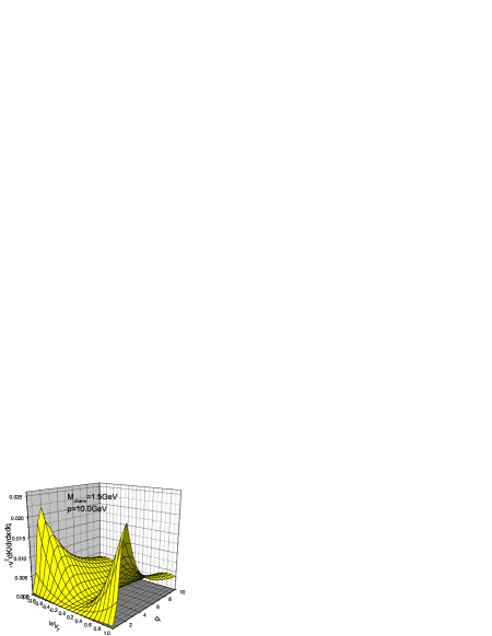
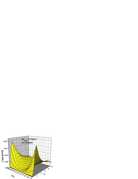
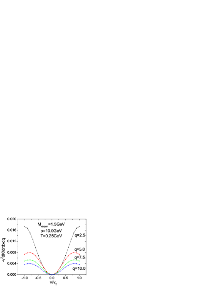
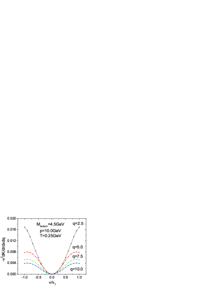
Figure 3: Surface plot of $-v^{2}dK/drdxdq$ for charm and bottom. See text.

Figure 4: $-v^{2}dK/drdxdq$ versus $v/v_{T}$ for charm and bottom quark for fixed $q$. See text.

VI Charm and Bottom Loss

Inserting (II.8) into (II.7) and using the explicit form (V.1) yields the energy loss in the SU(2) Coulomb plasma

$$-\frac{dK}{dr}= \frac{g^{2}\,C_{F}}{4\pi}\frac{\omega_{p}^{2}}{v^{2}}\int_{0}^{k_{max}}\,{dk}\,\frac{1}{k}\,$$

$$\times\frac{1}{\sqrt{2\pi}}\int_{-v/v_{T}}^{v/v_{T}}\,dx\,e^{x^{2}/2}\,\Bigg{(}\bigg{(}(1-n{\bf c}_{D1}(k))\,e^{x^{2}/2}/x+n{\bf c}_{D1}(k)\,\psi(x)\bigg{)}^{2}+\pi\,n^{2}{\bf c}^{2}_{D1}(k)/2\Bigg{)}^{-1}$$

For an SU(2) probe charge after the substitution $\boldsymbol{q}^{2}\rightarrow g^{2}C_{F}/4\pi$ with $C_{F}$ the SU(2) Casimir. We note that (LABEL:CB1) is cutoff in the infrared by the Debye wave number since ${\bf S}_{01}(k)\approx k^{2}/k_{D}^{2}$. So the main contribution to the energy loss in (LABEL:CB1) stems from the region $k>k_{D}$ for which the SU(2) plasmon is too broad to contribute as we noted earlier. Most of the loss stems from the metallic part of the SU(2) plasma which is the analogue as rescattering against the free thermal spectrum explicit in (V.8).

In Fig. 4 we display the integrand in (LABEL:CB1) versus the jet velocity $v/v_{T}$ and the dimensionless momentum $q=ka_{WS}$. This is a weighted plot of the longitudinal spectral function along the jet velocity. The two wings at small $q$ are the two plasmons peaks, which progressively turns into the thermal distribution at larger $q$. In Fig. 4 we show the same integrand for fixed $q$ versus the jet velocity $v/v_{T}$ normalized to the thermal velocity $V_{T}$. We note again the 2 plasmon poles around $v\approx v_{T}$ at small $q$. The vanishing of the termal distribution at $q=0$ follows from the extra $x^{2}$ weight arising from the denominator of (LABEL:CB1) for ${\bf c}_{D1}(k)\approx 0$ at large $k$.

Since the loss is colored with only $l=1$ contributing and is metallic with only $k>k_{D}$ contributing, we do not see colored Cherenkov radiation stemming from plasmon emission ruppert&muller , nor the ubiquitous Mach cone stemming from coupling to the sound mode casalderryetal . While the sound mode contributes to ${\bf S}$ in (III.6) it drops in the statistical averaging as only $l=1$ or plasmon channel contributes. The energy loss in the classical colored SU(2) Coulomb plasma is mostly metallic with $k>k_{D}$ and soundless due to the color quantum numbers of the fast moving probe charge.

A qualitative estimate for the energy loss follows by using ${\bf S}_{01}(k)\approx k^{2}/(k^{2}+k_{D}^{2})$ and saturating the integrand by $k>k_{D}$,

$$-\frac{dK}{dr}\approx\frac{g^{2}\,C_{F}}{4\pi}\frac{\omega_{p}^{2}}{v^{2}}\,\left(\sqrt{2\over\pi}\int_{0}^{v/v_{T}}\,x^{2}\,e^{-x^{2}/2}\right)\,\,\ln{\left(\frac{k_{max}}{k_{D}}\right)}$$ (VI.2)

The upper divergence is manifest in (LABEL:CB1) at $k\gg k_{D}$ since ${\bf S}_{01}(k)\approx 1$ and ${\bf c}_{D1}(k)\approx k_{D}^{2}/k^{2}$ through the generalized Ornstein-Zernicke equation for all Coulomb couplings. The upper cutoff $k_{max}\approx 2\gamma\,mv$ which is set by the maximum momentum transfer to the thermal particle of mass $m$ in the rest frame of the probe particle $M\gg m$. Typically $M$ is charm and bottom, while $m\approx gT$ in weak coupling and $m\approx\pi T$ in strong coupling for a QCD plasma near the critical point. For the former $v/v_{T}\approx v\sqrt{g}$ (weak coupling) while for the latter $v/v_{T}\approx v\sqrt{\pi}$ (strong coupling). For $v/v_{T}\gg 1$ (VI.2) reduces further to

$$-\frac{dK}{dx}\approx\frac{g^{2}\,C_{F}}{4\pi}\frac{\omega_{p}^{2}}{v^{2}}\,\,\ln{\left(\frac{2\gamma\,m\,v}{k_{D}}\right)}$$ (VI.3)

For the SU(2) colored Coulomb plasma. Aside from the Casimirs, this result is analogous to the energy loss in the classical and Abelian Coulomb plasma ichimaru ; thoma .

To assess the energy loss for varying Coulomb coupling $\Gamma=({g^{2}C_{2}}/{4\pi})({\beta}/{a_{WS}})$, we will rewrite the energy loss  (LABEL:CB1) as

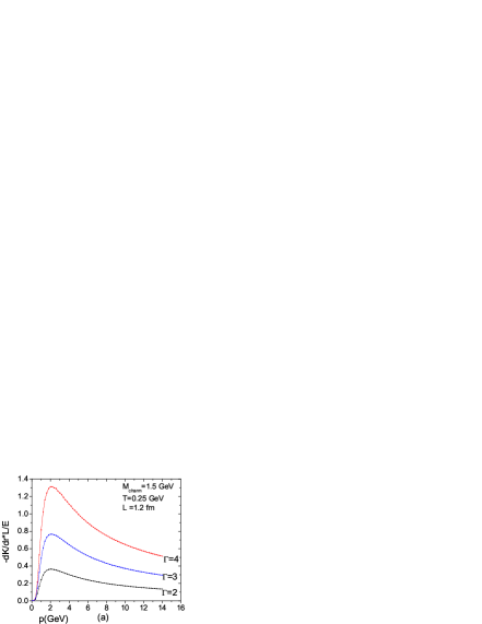
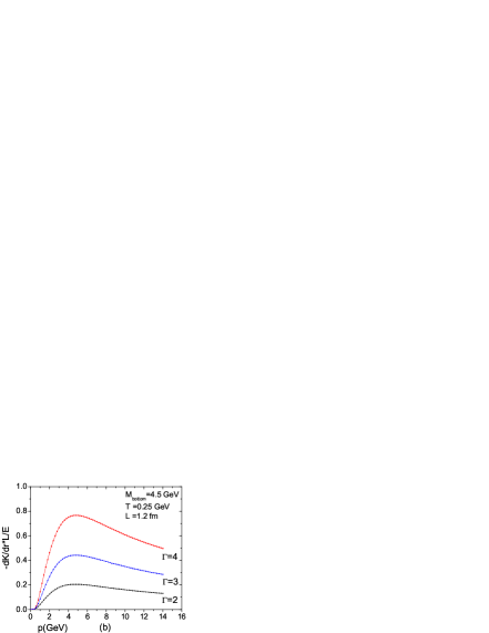
Figure 5: Energy loss for charm (left) and bottom (right) in the cQGP: $\Gamma=2,3,4$.

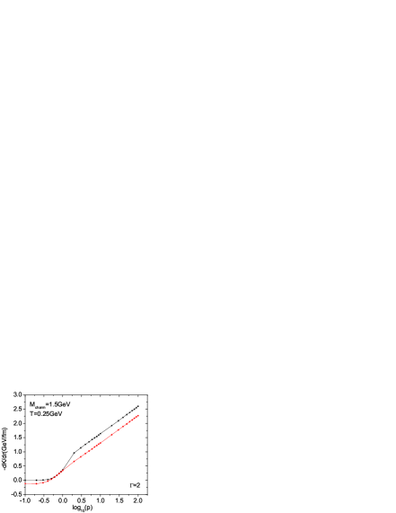
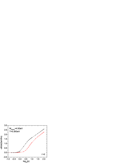
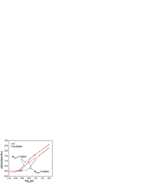
Figure 6: Logarithmic energy loss for charm (left) and bottom (right) in absolute units. See text.

$$-\frac{dK}{dr} = 3\Gamma^{2}\left(\frac{C_{F}}{C_{2}}\right)\frac{v_{T}^{2}}{v^{2}}\,\frac{T}{a_{WS}}\int_{0}^{q_{max}}\,{dq}\,\frac{1}{q}\,$$

$$\times \frac{1}{\sqrt{2\pi}}\int_{-v/v_{T}}^{v/v_{T}}\,dx\,e^{x^{2}/2}\,\Bigg{(}\bigg{(}(1-n{\bf c}_{D1}(q))\,e^{x^{2}/2}/x+n{\bf c}_{D1}(q)\,\psi(x)\bigg{)}^{2}+\pi\,n^{2}{\bf c}^{2}_{D1}(q)/2\Bigg{)}^{-1}$$

where $q=ka_{WS}$ and $a_{WS}$ is the Wigner-Seitz radius. The units for the energy loss per length in (LABEL:CB4) follows from $T/a_{WS}$. For SU(2), $C_{F}=3/4$ for a heavy quark, and $C_{2}=2$ for thermal constituent gluons of mass $m\approx\pi\,T$. $a_{WS}=({3}/{4\pi n})^{1/3}=(\frac{3}{4\pi}\frac{\beta^{3}}{0.244\times 3})^{1/3}=0.6883\beta$ for a density dominated by black-body (gluon) radiation $n=0.244(N_{c}^{2}-1)/\beta^{3}=0.244\times 3/\beta^{3}$.

In Fig. 5 we show the dimensionless energy loss following from (LABEL:CB4) for charm and bottom as a function of the probe momentum $\gamma Mv$, for different $\Gamma=2,3,4$ around the SU(2) liquid point. The numerics have been carried using the analytic structure factor of Fig. 1. The energy loss is normalized to the total kinetic energy in length $L$, $E/L=(\gamma-1)M/L$. Since the quark velocity is maintained constant, the energy loss is seen to exceed 1 for $\Gamma=4$. The loss is very sensitive to the Coulomb coupling $\Gamma$ in the liquid phase.

In Fig. 6 we show the energy loss on a logarithmic momentum scale for both charm and bottom. The upper curve (black) is the total loss from (LABEL:CB4), while the lower curve (red) is just the metallic loss following from (VI.3). The difference is a measure of the energy loss due to collisions with the low momentum part of the excitational spectrum of the SU(2) plasma which is plasmon dominated. These are the wings shown in Fig. 4. Charm and bottom jets with low momenta say $p\approx$ 3 GeV experience energy loss through broad plasmons. The energy loss for jets with $p$ larger than 10 GeV is mostly linear and therefore metallic.

In Fig. 7 we compare our analytical results for the energy loss (red curve) to recent SU(2) numerical simulations (black curve) using the same model dusling&zahed . We note that the numerical simulations in dusling&zahed are quoted for the mean-potential to kinetic energy ratio $V/K\approx 3$ which happens to fluctuate by about $\pm 1$ inside the simulation box. To make the comparison meaningful, it is better to use in the notation of dusling&zahed $\Gamma=1/Ta_{WS}\approx 4.8$ for $n=1/\lambda^{3}$ and $\lambda=1/3T$ with $\lambda$ the minimum of the potential in the same notations. With this in mind, our analytical results at $\Gamma=4$ compare favorably with the molecular dynamics simulations at large momenta and for heavier quark masses (say bottom). Most of the discrepancy with the simulations is at low momentum where the effects of the hard core in dusling&zahed are the largest.

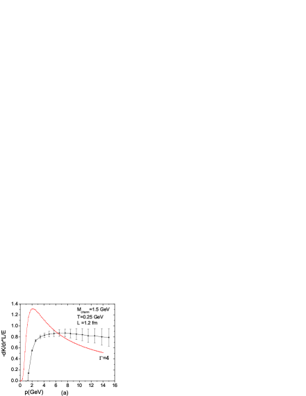
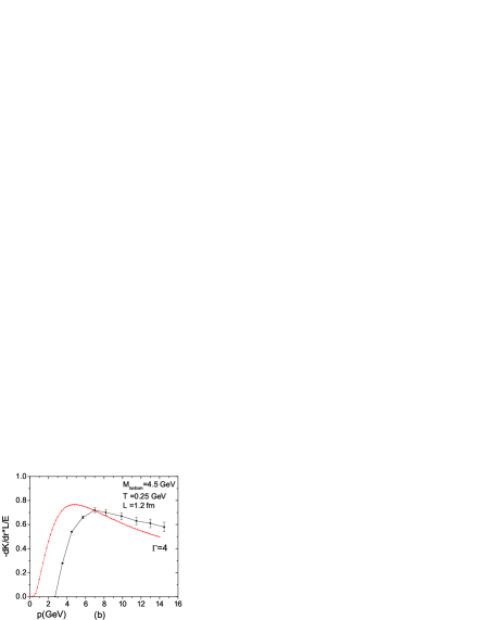
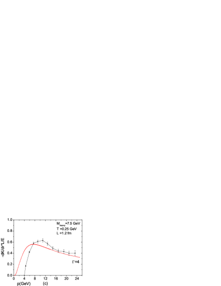
Figure 7: Energy loss: (red) analytical versus (black) SU(2) molecular dynamics dusling&zahed .

VII Conclusions

We have analyzed the energy loss of fast moving charm and bottom quarks in an SU(2) color Coulomb plasma for a broad range of the Coulomb coupling. The Coulomb character of the underlying interaction retained classically make the energy loss entirely described by the longitudinal part of the dielectric function. We have used linear response theory to derive an explicit expression for the imaginary part of the dielectric function in terms of the Laplace transform of the time-dependent structure factor in the SU(2) Coulomb plasma.

We have shown that the probe initial color and statistical averaging causes the longitudinal dielectric function to select the $l=1$ color channel of the time-dependent structure factor which is the plasmon channel. The sound channel dominates the low momentum of the $l=0$ color channel, and decouples from the longitudinal part of the dielectric function. While the SU(2) plasmon survives at strong coupling, its width for $k>k_{D}$ is substantial and therefore causes it to thermally decay.

The energy loss of fast moving charm and bottom quarks is mostly due to the metallic aspect of the SU(2) colored Coulomb plasma which is dominated by thermal particles. There is no colored Cerenkov cone as the plasmon is dwarfed in the metallic limit, nor a colorless Mach cone as the sound decouples due to the probe initial colors. The energy loss is soundless. Our results are of course only classical. They apply for a broad range of $\Gamma$ near the liquid point. The comparison to the MD simulations show that our energy loss is about comparable at higher momenta and for heavier quarks where the effects of the numerical hard core is small. As initially reported in dusling&zahed , the energy loss is sizable.

Strong coupling assessment of jet energy loss in gauge theories have been carried out in the context of holographic QCD herzogetal . The fact that a Mach cone was reported in these calculations chesler&yaffe , maybe due to the fact that the probe jet is actually colorless. Indeed, most of the holographic jets are inserted with an external hand that maintains a constant velocity and perhaps even balance the color charge. Clearly colorless (mesonic) jets of the type $\overline{Q}Q$ do couple to the sound channel in our case through the ${\bf S}_{00}(k)$ structure factor cho&zahed3 , and are expected to be trailed by a Mach cone.

Finally, to carry our analysis of charm and bottom at RHIC and perhaps even LHC, require an assessment of the heavy quark composition in the prompt phase of the heavy ion collision which we have not carried out. Also, we need to address more carefully the correspondence between our classical SU(2) QGP and the quantum SU(3) QGP. These issues will be addressed next.

- (1) E. V. Shuryak, Prog. Part. Nucl. Phys. 62, 48 (2009)
- (2) M. H. Thoma and M. Gyulassy, Nucl. Phys. B 351, 491 (1991)
- (3) E. Braaten and M. H. Thoma, Phys. Rev. D 44, 1298 (1991)
- (4) E. Braaten and M. H. Thoma, Phys. Rev. D 44, R2625 (1991)
- (5) M. Djordjevic, Phys. Rev. C 74, 064907 (2006)
- (6) M. Djordjevic and U. Heinz, Phys. Rev. Lett. 101, 022302 (2008)
- (7) M. Djordjevic and U. Heinz, Phys. Rev. C 77, 024905 (2008)
- (8) A. Dumitru, Y. Nara, B. Schenke and M. Strickland, Phys. Rev. C 78, 024909 (2008)
- (9) S. Sin and I. Zahed, Phys. Lett. B 608, 265 (2005)
- (10) H. Liu, K. Rajagopal and U. A. Wiedemann, Phys. Rev. Lett. 97, 182301 (2006)
- (11) B. A. Gelman, E. V. Shuryak and I. Zahed, Phys. Rev. C 74, 044908 (2006)
- (12) B. A. Gelman, E. V. Shuryak and I. Zahed, Phys. Rev. C 74, 044909 (2006)
- (13) S. Cho and I. Zahed, Phys. Rev. C 79, 044911 (2009)
- (14) S. Cho and I. Zahed, Phys. Rev. C 80, 014906 (2009)
- (15) K. Dusling and I. Zahed, arXiv:0904.0169
- (16) S. Ichimaru, Statistical Plasma Physics Vol I:Basic Principles (Westview Press, 2004)
- (17) S. Cho and I. Zahed, arXiv:0909.4725
- (18) S. Cho and I. Zahed, arXiv:0910.2666
- (19) M. H. Thoma, J. Phys. G 26, 1507 (2000)
- (20) J. Ruppert and B. Muller, Phys. Lett. B 618, 123 (2005)
- (21) J. Casalderrey-Solana, E. V. Shuryak and D. Teaney, Nucl. Phys. A 774, 577 (2006)
- (22) C. P. Herzog, A. Karch, P. Kovtun, C. Kozcaz and L. G. Yaffe, JHEP. 07, 013 (2006)
- (23) P. M. Chesler and L. G. Yaffe, Phys. Rev. Lett. 99, 152001 (2007)