Ly$\alpha$ versus X-ray heating in the high-z IGM

Abstract

In this paper we examine the effect of X-ray and Ly$\alpha$ photons on the intergalactic medium temperature. We calculate the photon production from a population of stars and micro-quasars in a set of cosmological hydrodynamic simulations which self-consistently follow the dark matter dynamics, radiative processes as well as star formation, black hole growth and associated feedback processes. We find that, (i) IGM heating is always dominated by X-rays unless the Ly$\alpha$ photon contribution from stars in objects with mass $M<10^{8}$ M_⊙ becomes significantly enhanced with respect to the X-ray contribution from BHs in the same halo (which we do not directly model). (ii) Without overproducing the unresolved X-ray background, the gas temperature becomes larger than the CMB temperature, and thus an associated 21 cm signal should be expected in emission, at $z\lower 2.15277pt\hbox{$\;\buildrel<\over{\sim}\;$}11.5$. We discuss how in such a scenario the transition redshift between a 21 cm signal in absorption and in emission could be used to constraint BHs accretion and associated feedback processes.

1 Introduction

While the investigation of the very high-$z$ universe, $z\sim 1000$, is possible through the Cosmic Microwave Background (CMB) radiation and detection of a handful of objects with redshift as high as $\sim 7$ has recently been possible, there is a lack of observational data in the redshift interval $7\lower 2.15277pt\hbox{$\;\buildrel<\over{\sim}\;$}z\lower 2.15277pt\hbox{$\;\buildrel<\over{\sim}\;$}1000$. To detect radiation from this interval, telescopes with exceptional sensitivity in the IR and radio bands are needed. JWST (James Webb Space Telescope), for example, with its nJy sensitivity in the $1-10$ $\mu$m infrared regime, is ideally suited for probing optical-UV emission from sources at $z>10$. Similarly, the planned generation of radio telescopes as SKA (Square Kilometer Array), LOFAR (LOw Frequency ARray), 21cmA (21cm Array) and MWA (Murchison Widefield Array) will open a new observational window on the high redshift universe. In particular, the detection of the 21 cm line associated with the hyperfine transition of the ground state of neutral hydrogen, holds the promise to shed light on the reionization process and its sources.

This observational progress has been accompanied by a flourishing of theoretical activity, aimed at providing predictions for the planned generation of telescopes. It has long been known (e.g. Field 1959) that neutral hydrogen in the intergalactic medium (IGM) and gravitationally collapsed systems may be directly detectable in emission or absorption against the CMB at the frequency corresponding to the redshifted HI 21 cm line (associated with the spin-flip transition from the triplet to the singlet ground state). Madau et al. (1997) first showed that 21 cm tomography could provide a direct probe of the era of cosmological reionization and reheating. In general, 21 cm spectral features will display angular structure as well as structure in redshift space due to inhomogeneities in the gas density field, hydrogen ionized fraction, and spin temperature. Several different signatures have been investigated in the recent literature among which fluctuations in the 21 cm line emission induced by the “cosmic web” (Tozzi et al., 2000), by the neutral hydrogen surviving reionization (e.g. Ciardi & Madau 2003; Furlanetto et al. 2004; Mellema et al. 2006) and a global feature (“reionization step”) in the continuum spectrum of the radio sky that may mark the abrupt overlapping phase of individual intergalactic HII regions (Shaver et al., 1999).

A key feature for the observation of the line in emission is that the IGM should be heated above the CMB temperature. While pre-heating can happen due to, e.g., dark matter particles decay or annihilation (e.g. Mapelli et al. 2006; Valdés et al. 2007), the main source of heating are Ly$\alpha$ and X-ray photons. Although the impact of these sources has been investigated by several authors (e.g. Madau et al. 1997; Chen & Miralda-Escudé 2004; Nusser 2005; Kuhlen et al. 2006; Ciardi & Salvaterra 2007; Pelupessy et al. 2007; Ripamonti et al. 2008), none of the above studies has approached the problem considering both sources within a self-consistent model. Here, we estimate the Ly$\alpha$ and X-ray photon production using the simulations by Pelupessy et al. (2007), which were designed to follow the evolution of both quasar and stellar type sources, including their associated feedback effects. The above estimates are then used to calculate with a semi-analytic approach the evolution of the temperature of an IGM at the mean density.

The paper is structured as follows. In Section 2 we describe the main characteristics of the simulations by Pelupessy et al. (2007), while in Section 3 we give the prescription used to derive the Ly$\alpha$ and X-ray photon count. In Section 4 we estimate the IGM heating due to the emitted photons, in Section 5 the consequences for the observability of the 21 cm line from neutral hydrogen and in Section 6 we give our conclusions.

2 Simulations of halo collapse and black holes growth

As mentioned in the Introduction, in this paper we make use of the simulations described in Pelupessy et al. (2007). Here we briefly outline the main characteristics and we refer the reader to the original paper for details.

The simulations are designed to investigate the physical conditions for the growth of intermediate mass seed black holes (BHs; possibly the remnants of a first generation of massive stars), using the parallel cosmological TreePM-Smooth Particle Hydrodynamics (SPH) code GADGET2 (Springel, 2005) in the standard $\Lambda$CDM model. The initial conditions for the simulation correspond to isolated spherical overdensities (’top-hat’) endowed with an appropriate Zeldovich power spectrum (similar to Bromm & Larson 2004). During collapse of the parent halo (all halos considered have $T_{\rm vir}>10^{4}$ K) the seed holes are incorporated through mergers into larger systems and accrete mass from the surrounding gas. The interstellar medium (ISM), star formation and supernovae feedback as well as black hole accretion and associated feedback are treated self-consistently by means of sub-resolutions models. In particular, the multiphase model for star forming gas has been developed by Springel & Hernquist (2003), while the prescription for accretion and feedback from massive black holes is the one developed by Di Matteo et al. (2005) and Springel et al. (2005). Technically, black holes are represented by collisionless particles that grow in mass by accreting gas from their environments. The (unresolved) accretion onto the black hole is related to the large scale (resolved) gas distribution using a Bondi-Hoyle-Lyttleton parameterization (Bondi, 1952; Bondi & Hoyle, 1944), and it is limited by the Eddington rate. A fraction $\epsilon_{\rm f}$ of the radiative energy released by the accreted material is assumed to couple thermally to nearby gas. In addition, two black hole particles are assumed to merge if they come within the spatial resolution of the simulation (i.e. within the local SPH smoothing length) and their relative speed lies below the local sound speed. The seeding procedure constists in selecting objects with a mass of $10^{6}$ M_⊙ and place a seed BH of $M_{\rm seed}=10^{3-4}$ M_⊙ in them if they do not already contain a BH.

Different collapse scenarios have been investigated by choosing the total mass $M$ of the host halos, the redshift of collapse $z_{\rm vir}$ and the spin parameter $\lambda$. The halos considered have a mass of $M=10^{8},10^{9},10^{10}$ and $10^{11}$ M_⊙, with a virialization redshift of $z_{\rm vir}=16,12,10$ and $7.5$, respectively. A standard spin parameter of $\lambda=0.03$ is adopted, but simulations with $\lambda=0$ or $\lambda=0.05$ have determined no significant difference in the results (Pelupessy et al., 2007). The simulations used here are the highest resolution ones, having $N=10^{7}$ particles (in dark matter and gas), with a corresponding spatial resolution of a about hundred parsec. Two extreme values for the BH feedback have been considered: $\epsilon_{\rm f}=0$ corresponding to the case without any black hole feedback (this can be used for comparison) and $\epsilon_{\rm f}=0.5$, the value that has been used to reproduce the observed normalization of the local $M_{\rm BH}$-$\sigma$ relation in galaxy merger simulations (Di Matteo et al., 2005) as well as in full cosmological hydrodynamical simulations where the same modeling was applied (Di Matteo et al., 2008). All simulations here are run to a final redshift of $z\sim 6$.

Despite the analysis of a quite broad parameter space, the simulations do not account for possible effects associated with gravitational recoil (for a thourough discussion on the implications we refer the reader to the original paper).

The simulations are used to derive the X-ray and Ly$\alpha$ photon production as described in the following Section.

3 Photon count

In this Section we discuss our estimate of the X-ray and Ly$\alpha$ photon production and associated background. Our reference run has $M_{\rm seed}=10^{4}$ M_⊙, $\lambda=0.03$, $\epsilon_{\rm f}=0.5$.

The bolometric luminosity associated to a BH accreting at a rate $\dot{M}_{\rm BH}(z,M_{h})$ hosted in a halo of mass $M_{h}$ at redshift $z$ is $L(z,M_{h})=\epsilon c^{2}\dot{M}_{\rm BH}(z,M_{h})$, where $\epsilon=0.1$ is the radiative efficiency for accretion (for a Shakura-Sunyaev, and non-spinning black hole) and $c$ is the speed of light. The comoving specific emissivity at redshift $z$ is then:

$$j_{\rm BH}(\nu,z)=\int_{M_{h,min}}^{M_{h,max}}\frac{l_{\rm BH}(\nu,z)}{\int l_{\rm BH}(\nu^{\prime},z)d\nu^{\prime}}L(z,M_{h})n_{\rm PS}(z,M_{h})dM_{h},$$ (1)

where $n_{\rm PS}(z,M_{h})$ is the weight for the halo of mass $M_{h}$ at redshift $z$ as computed by the Press-Schechter formalism, and $M_{h,min}$ and $M_{h,max}$ are the minimum and maximum masses for our simulated halo mass, respectively. $M_{h,min}$ is set by the physics appropriately captured in the simulations, which do not follow the chemistry of molecular hydrogen. $l(\nu,z)$ is the average spectrum energy distribution for AGNs as computed by Sazonov et al. (2004).

The total cosmic star formation rate density at redshift $z$ is:

$$\dot{\rho}_{\star}(z)=\int_{M_{h,min}}^{M_{h,max}}\dot{M}_{\star}(z,M_{h})n_{\rm PS}(z,M_{h}),$$ (2)

where $\dot{M}_{\star}(z,M_{h})$ is the star formation rate for the halo of mass $M_{h}$ at redshift $z$.

For stars, the comoving specific emissivity is computed by:

$$j_{\star}(\nu,z)=\int_{z}^{\infty}dz^{\prime}l_{\star}(\nu,t_{z,z^{\prime}})\dot{\rho}_{\star}(z),$$ (3)

where $l_{\star}(\nu,t_{z,z^{\prime}})$ is the template specific luminosity for a stellar population of age $t_{z,z^{\prime}}$ (time elapsed between redshift $z^{\prime}$ and $z$) as computed by Bruzual & Charlot (2003) for Pop II stars with $Z=0.2\;Z_{\odot}$ and a Salpeter IMF. In Ciardi & Salvaterra (2007) it was shown that, although the ionizing photon production is much reduced (by a factor of $\sim 4$) compared to metal-free stars with the same IMF, the Ly$\alpha$ photon emission is similar. For this reason we limit our discussion to metal enriched stars.

The background intensity $J(\nu_{0},z_{0})$ seen at a frequency $\nu_{0}$ by an observer at redshift $z_{0}$ is then given by:

$$J(\nu_{0},z_{0})=\frac{(1+z_{0})^{3}}{4\pi}\int^{\infty}_{z_{0}}j(\nu,z)e^{-\tau(\nu_{0},z_{0},z)}\frac{dl}{dz}dz,$$ (4)

where $\nu=\nu_{0}(1+z)/(1+z_{0})$, $dl/dz$ is the proper line element, and $j(\nu,z)=j_{\star}(\nu,z)+j_{\rm BH}(\nu,z)$ is the total emissivity. $\tau(\nu_{0},z_{0},z)$ is the optical depth of the medium.

For Ly$\alpha$ photons, $\tau$ as been computed as in Salvaterra & Ferrara (2003, see Sect. 2.2 for a full description of the IGM modeling). The evolution of the Ly$\alpha$ background is shown in Figure 1. We note that its intensity is much smaller than what found in Ciardi & Salvaterra (2007). This effect can be attributed to the larger $M_{h,min}$ employed here, as set by the smallest simulated halos.

In the X-rays,

$$\tau(\nu,z_{0},z)=\int_{z_{0}}^{z}\frac{dl}{dz}\sigma\left(\nu\frac{1+z^{\prime}}{1+z_{0}}\right)n_{B}(z^{\prime}),$$ (5)

where $\sigma(\nu)$ is the photon-ionization cross section per baryon of a cosmological mixture of H and He (Zdziarski & Svensson 1989; see also Ripamonti et al. 2008 for a more thorough discussion) and $n_{B}(z)=n_{B}(0)(1+z)^{3}$ is the cosmological baryon number density at redshift $z$ ($n_{B}(0)\simeq 2.5\times 10^{-7}$ cm^-3; Spergel et al. 2007). Here, we neglect the stellar contribution to the X-ray background which is negligible with respect to the AGN one (see also Oh 2001), so that $j(\nu,z)=j_{\rm BH}(\nu,z)$. The evolution of the X-ray background at $\nu_{0}=150$ eV (dashed line) and 1 keV (dashed-dotted) is shown in Figure 1. Even though a detailed comparison is beyond the scope of this paper, we note that our results here are overall consistent with those of Ripamonti et al. (2008) who used a set of semi-analitical models to study X-ray heating from early black holes.

A strong upper limit to the AGN activity at high redshift is set by the unresolved fraction of the observed cosmic X-ray background (Salvaterra et al., 2007). To make sure our mini-quasar population does not conflict with this requirement, we compute the contribution of our simulated BHs to the observed diffuse cosmic X-ray background in the 0.5-2 keV and 2-8 keV bands. We find that this contribution is $\sim 0.9\times 10^{-12}$ and $\sim 1.8\times 10^{-12}$ erg s^-1 cm^-2 deg^-2, respectively, that is $\sim 40$% of the most recent estimates of the unresolved fraction (Hickox & Markevitch, 2007; Moretti et al., 2009). Even considering the expected contribution of faint, $z<4$ AGNs missed by current deep surveys (Volonteri et al., 2006), our calculation implies values well below the observational limits.

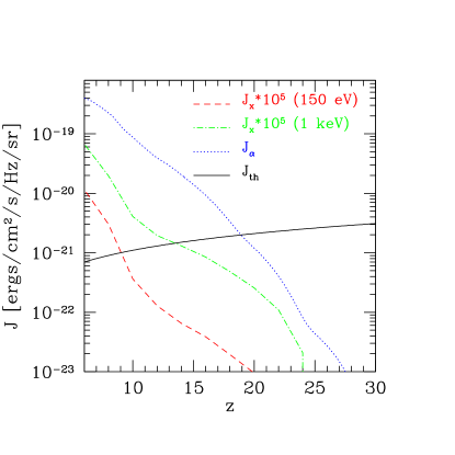
Figure 1: Evolution of the Ly$\alpha$ (dotted line), X-ray at 150 eV (dashed) and 1 keV (dashed-dotted) background radiation. The solid line is the minimum intensity required for the Ly$\alpha$ background to be effective in decoupling the spin temperature from $T_{\rm CMB}$.

4 IGM heating

Results from previous studies (e.g. Madau et al. 2004) have shown that photons with energies $h\nu>150$ eV typically have a mean free path larger than the average separation between sources; it is possible therefore to divide the radiation field in a fluctuating component with 13.6 eV$<h\nu<150$ eV (which creates expanding patchy HII regions), and a nearly uniform soft X-ray background component with 150 eV$<h\nu<2$ keV (which ionizes the IGM homogeneously). Here we concentrate on the effect of the latter component on the thermal evolution of the IGM.

We can calculate the energy rate per H atom (in units of [erg s^-1]) at redshift $z$ as:

$$\dot{E}_{x}(z)=4\pi\int_{150{\rm eV}}^{2{\rm keV}}J(E,z)\sigma(E)dE,$$ (6)

where $J(E,z)$, with $E=h\nu$, is computed by eq. 4.

Of the above energy, a fraction $f_{heat}$ goes into heating of the IGM and a fraction $f_{ion}$ goes into H ionization (Shull & van Steenberg 1985; Valdés & Ferrara 2008) . We have verified that by using the two parameterizations of $f_{heat}$ the overall discrepancy in our results (in terms of IGM temperature) is at most a few percent. In the following, we adopt the results by Valdés & Ferrara (2008).

The evolution of the IGM temperature, $T_{IGM}$, is followed as in Ciardi & Salvaterra (2007) (based on Chuzhoy & Shapiro 2007), i.e. $T_{IGM}$ is calculated with RECFAST (Seager et al., 1999) until the first sources of radiation turn on. Subsequentely, taking into account the presence of the heating from X-ray photons and neglecting the contribution from deuterium, which turned out to be negligible, the evolution of $T_{IGM}$ is regulated by:

$$\frac{dT_{IGM}}{dt}=\frac{2}{3k}\left(H_{\alpha}+H_{x}\right)-\frac{4T_{IGM}}{3t}.$$ (7)

Here $H_{\alpha}$ and $H_{x}=f_{heat}(z,x_{\rm HII})\dot{E}_{x}(z)$ are the heating rates per H atom due to Ly$\alpha$ and X-ray photons, respectively. We refer the reader to the original paper (Ciardi & Salvaterra 2007) for the derivation of $H_{\alpha}$. $\dot{N}_{\alpha}$ (the number of photons that pass through the Ly$\alpha$ resonance per H atom per unit time) necessary to calculate $H_{\alpha}$ has been derived from the model described in the previous Section.

It should be noted that the impact of Ly$\alpha$ photon scattering on the evolution of the IGM temperature has been recently revised by e.g. Chen & Miralda-Escudé (2004), Hirata (2006), Pritchard & Furlanetto (2006) and Chuzhoy & Shapiro (2007). Chen & Miralda-Escudé (2004) included atomic thermal motion in their calculations, finding a heating rate several orders of magnitude lower than the previous estimate by Madau et al. (1997). In addition, while “continuum” photons (with frequency between the Ly$\alpha$ and Ly$\beta$) heat the gas, “injected” photons (which cascade into the Ly$\alpha$ from higher atomic resonances) cool the gas, resulting in an effective cooling from Ly$\alpha$ photons at temperatures above 10 K. Chuzhoy & Shapiro (2007) though, showed that the cascade which follows absorption of photons in resonances higher than the Ly$\alpha$ happens via the 2s level rather than the 2p level. Thus, the number of “injected” photons and their cooling efficiency are reduced compared to the estimate of Chen & Miralda-Escudé (2004) and Ly$\alpha$ photon scattering can be an efficient heating source also at temperatures higher than 10 K. Here we follow the calculation of Chuzhoy & Shapiro (2007).

As $H_{x}$ is also a function of the ionization fraction, eq. 7 needs to be solved together with the following equation:

$$\frac{dx_{\rm HII}}{dt}=f_{ion}(t,x_{\rm HII})\dot{N}_{x}\frac{n_{\rm H}}{n_{\rm HI}}+k_{coll}n_{e}x_{\rm HI}-k_{rec}n_{e}x_{\rm HII},$$ (8)

where $x_{\rm HII}$ and $x_{\rm HI}$ are the HII and HI fraction respectively, $n_{\rm H}$ and $n_{\rm HI}$ are the number density of H and HI respectively, $k_{coll}$ and $k_{rec}$ are the collisional and recombination rates, $\dot{N}_{x}$ is the rate of X-ray photons per H atom.

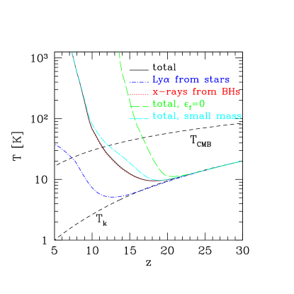
Figure 2: Temperature evolution as a function of redshift: total (solid black line), total in the absence of black holes feedback (long-dashed green line), total with an extension to lower masses of the contribution of stellar type sources (long-dashed-dotted cyan line) as determined by X-ray heating from black holes only (dotted red line) and by Ly$\alpha$ photons from stars only (short-dashed-dotted blue line). The upper (lower) dashed curve is the CMB temperature (the IGM temperature in the absence of any heating mechanisms).

In Figure 2 the evolution of the IGM temperature as given by eqs. 7 and 8 is shown, together with the CMB temperature, $T_{\rm CMB}$, and the IGM temperature, $T_{k}$, in the absence of any heating mechanisms. The solid curve includes the contribution to the heating of X-rays from BHs, Ly$\alpha$ photons from both BHs and stars. It is clear from the Figure that the contribution from the Ly$\alpha$ photons is irrelevant for the evolution of the IGM temperature, which is instead dominated by the X-ray heating (see Sec 6 for a more extensive discussion). We note that the contribution to the Ly$\alpha$ photons from the BHs is negligible compared to that from the stars.

5 Spin and differential brightness temperature

As the physics behind the emission/absorption of the 21 cm line has been discussed extensively by several authors (for a review see e.g. Furlanetto et al. 2006), here we just write the relevant equations, following Ciardi & Salvaterra (2007). The evolution of the spin temperature, $T_{s}$, can be written as Chuzhoy & Shapiro (2006):

$$T_{s}=\frac{T_{\rm CMB}+(y_{\alpha,eff}+y_{c})T_{\rm IGM}}{1+y_{\alpha,eff}+y_{c}},$$ (9)

where $T_{\rm CMB}$ is the CMB temperature;

$$y_{c}=\frac{T_{\star}}{A_{10}T_{\rm IGM}}(C_{\rm H}+C_{e}+C_{p}),$$ (10)

is the coupling efficiency due to collisions with H atoms, electrons and protons, $T_{\star}=0.068$ K is the temperature corresponding to the energy difference between the singlet and triplet hyperfine levels of the ground state of neutral hydrogen and $A_{10}=2.85\times 10^{-15}$ s^-1 is the spontaneous emission rate. For the de-excitation rates $C_{\rm H}$, $C_{e}$ and $C_{p}$ we have adopted the fits used by Kuhlen, Madau & Montgomery (2006; see also the original papers by Smith 1966; Allison & Dalgarno 1969; Liszt 2001; Zygelman 2005), i.e. $C_{\rm H}=n_{\rm H}\kappa$, $C_{e}=n_{e}\gamma_{e}$ and $C_{p}=3.2n_{p}\kappa$ with $n_{\rm H}$, $n_{e}$, $n_{p}$ hydrogen, electron and proton number density, $\kappa=3.1\times 10^{-11}T_{\rm IGM}^{0.357}{\rm exp}(-32/T_{\rm IGM})$ cm³ s^-1 and ${\rm log}(\gamma_{e}/1{\rm cm}^{3}{\rm s}^{-1})=-9.607+0.5{\rm log}(T_{\rm IGM}){\rm exp}[-({\rm log}T_{\rm IGM})^{4.5}/1800]$. Finally,

$$y_{\alpha,eff}=y_{\alpha}{\rm e}^{-0.3(1+z)^{1/2}T_{\rm IGM}^{-2/3}}\left(1+\frac{0.4}{T_{\rm IGM}}\right)^{-1},$$ (11)

is the effective coupling efficiency due to Ly$\alpha$ scattering which takes into account the back-reaction of the resonance on the Ly$\alpha$ spectrum and the effect of resonant photons other than Ly$\alpha$, and $y_{\alpha}=P_{10}T_{\star}/(A_{10}T_{\rm IGM})$, with $P_{10}\sim 10^{9}J_{\alpha}$ s^-1 radiative de-excitation rate due to Ly$\alpha$ photons.

In the upper panel of Figure 3 the spin temperature is shown as a function of redshift together with $T_{\rm CMB}$ and the IGM temperature in the absence of heating mechanisms $T_{k}$ (upper and lower dashed lines, respectively). As the intensity required for a Ly$\alpha$ background to be effective in decoupling the spin temperature from $T_{\rm CMB}$ is $J_{\alpha}\lower 2.15277pt\hbox{$\;\buildrel>\over{\sim}\;$}10^{-22}(1+z)$ ergs cm^-2 s^-1 Hz^-1 sr^-1 (e.g. Ciardi & Madau 2003, see Fig. 1), $T_{s}$ gets coupled to $T_{\rm IGM}$ as early as $z\sim 19$, but only at $z\sim 11$ does it become larger than $T_{\rm CMB}$ due to X-ray heating.

The differential brightness temperature, $\delta T_{b}$, between the CMB and a patch of neutral hydrogen with optical depth $\tau$ and spin temperature $T_{s}$ at redshift $z$, can be written as:

$$\delta T_{b}=(1-{\rm e}^{-\tau})\frac{T_{s}-T_{\rm CMB}}{1+z}.$$ (12)

For a gas at the mean IGM density, the optical depth is:

$$\tau(z)=\frac{3A_{10}\lambda^{3}}{32\pi}\frac{T_{\star}}{T_{s}}\frac{n_{\rm HI}(z)}{H(z)},$$ (13)

where $\lambda$ is the wavelength of the transition, $n_{\rm HI}$ is the number density of neutral hydrogen and $H(z)$ is the Hubble constant.

In the lower panel of Figure 3 $\delta T_{b}$ is plotted for the spin temperature calculated above, reflecting its behavior, with a signal in emission (absorption) expected for $z\lower 2.15277pt\hbox{$\;\buildrel<\over{\sim}\;$}(\lower 2.15277pt\hbox{$\;\buildrel>\over{\sim}\;$})11$.

Figure 3: Upper panel: Evolution of the spin temperature (solid line). $T_{\rm CMB}$ and the IGM temperature in the absence of heating mechanisms, $T_{k}$, are plotted as upper and lower dashed lines, respectively. Lower panel: Evolution of the differential brightness temperature. Lines are the same as in the upper panel.

6 Discussion and summary

In this paper we have estimated the effect of X-ray and Ly$\alpha$ photons on the IGM temperature. This was done calculating the photon production from a population of both stars and quasars based on the self-consistent modeling of these sources and associated feedback processes in the simulations by Pelupessy et al. (2007). Such photon production has then been used to determine the evolution of the IGM temperature with a semi-analytic approach. The calculations assume a gas at the mean density whose ionization history is regulated by the effect of the X-ray photons. Thus, they are strictly valid as long as the filling factor of gas ionized by UV photons is small or in regions of the IGM that have not been reached by UV-ionizing radiation. For reference, the filling factor of ionized regions, under the assumption that it is independent from the effect of the X-rays, assuming a gas clumping factor of 10 and an escape fraction of ionizing photons from stellar type sources of 10% is $\sim 0.004,0.07,1$ at $z=15,10,7.1$. It should be noted here that the bulk of the UV photons is produced by stars rather than BHs, while the contribution to the ionization fraction from X-rays is only a few percents.

The results presented of course depend quite strongly on the parameters and assumptions adopted in the simulations described in Section 2. As already mentioned, while e.g. the value of the spin parameter has a negligible effect on the final outcome, the presence of AGN feedback (but not the specific value of $\epsilon_{f}$, as long as $\neq 0$) is crucial. In our reference run we have used a vale $\epsilon_{f}=0.5$, which corresponds to coupling only $5\%$ of the radiated energy. In Pelupessy et al. (2007) we have shown that no significant difference in the BH accretion rates are seen for $\epsilon_{f}=0.5$, but that of course cases with $\epsilon_{f}=0$ can imply much larger accretion rates (and associated X-ray photons). For the sake of illustration, we have performed the same calculations also for the extreme case without feedback, i.e. for $\epsilon_{f}=0$. Note that for our calculation this is a completely unrealistic model, which we consider only as a parametric study. The result is shown in Figure 2 as long-dashed line. As expected, the value of the IGM temperature raises much more quickly than in the reference case and becomes larger than $T_{\rm CMB}$ already at $z\sim 16$. This would result also in an earlier 21 cm signal in emission. This case is both unrealistic and also results in a contribution to the unresolved X-ray background which is orders of magnitudes larger than the available observational limits and thus can be discarded.

So it remains that our results depend most strongly on the choice of $M_{h,min}$ and $M_{h,max}$ in eqs. 1 and 2, which in our case we have taken from the masses of the simulated halos. While larger values of $M_{h,max}$ are expected to have a negligible impact because of the paucity of such objects at the redshifts of interest, a smaller $M_{h,min}$ (and its associated high abundance) would result in higher photon production. While extending eq. 2 to smaller masses is straightforward, it may not be appropriate as the contribution from these low mass halos depends on more complicated forms and strength of the feedback active in the relevant range of redshift (for a review on feedback see Ciardi & Ferrara 2005). Although a consensus on the detailed effects of feedback (in particular radiative feedback) on small structure formation has not been reached yet, most authors agree that the presence of feeback delayes or suppresses the formation of small mass objects, and thus associated star formation, depending on a variety of physical quantities such as redshift, halo mass and molecular hydrogen content (see e.g. Machacek et al. 2001; Susa & Umemura 2006; O’Shea & Norman 2007; Whalen et al. 2008). A proper treatment of such feedback though is beyond the scope of the present paper. Similarly the emission properties of mini-QSOs hosted in such small halos is largely unknown and may not be described by the average AGN spectrum here adopted. Thus, we have neglected the contribution of these objects to the total X-ray photon production (see Madau et al. 2004; Dijkstra et al. 2004; Salvaterra et al. 2005 for a discussion about the effect of mini-QSOs in the early universe).

As a reference though, an upper limit for the contribution of Ly$\alpha$ photon to the IGM temperature is plotted in Figure 2. Here (long-dashed-dotted cyan line) we show the effects accounting for the contribution to the star formation rate of objects with mass as small as $10^{7}$ M_⊙. As expected, in this case, the IGM temperature starts to raise at an earlier time due to Ly$\alpha$ heating and becomes larger than $T_{\rm CMB}$ at $z\sim 12$, while X-ray photons dominate heating at $z\lower 2.15277pt\hbox{$\;\buildrel<\over{\sim}\;$}10$. Note however, this considers that these halos will not produce any X-ray photons, i.e. the accretion onto their black holes must be completely quenched. This is likely a conflicting requirement, as both star formation and black hole accretion will somewhat depend on the same gas supply. To summarize this point, in order to have 21 cm line in emission, X-ray heating from BHs and/or extremely efficient star formation (albeit, as discussed above, somewhat unfeasible) in halos with $M_{h}<10^{8}M_{\odot}$ is required. The heating due to stars only in larger halos as shown in Figure 2, is however unable to bring the gas temperature above $T_{\rm CMB}$ before the reionization is completed.

To summarize the main results of this work, we find that:

• unless the Ly$\alpha$ photon contribution from stars in small mass objects is somehow strongly enhanced in comparison to the X-ray contribution from BHs in the same objects, the IGM heating is always dominated by X-rays;

• in this case, the transition redshift between a 21 cm signal in absorption and in emission could be used to constraint BHs accretion properties;

• for a case consistent with the available limits on the unresolved fraction of the X-ray background in the 0.5-2 keV and 2-8 keV bands, the IGM temperature becomes larger than the CMB temperature (and thus an associated 21 cm signal should be expected in emission) at $z\lower 2.15277pt\hbox{$\;\buildrel<\over{\sim}\;$}11.5$.

References

- Allison & Dalgarno (1969) Allison A. C., Dalgarno A., 1969, ApJ, 158, 423
- Bondi (1952) Bondi H., 1952, MNRAS, 112, 195
- Bondi & Hoyle (1944) Bondi H., Hoyle F., 1944, MNRAS, 104, 273
- Bromm & Larson (2004) Bromm V., Larson R. B., 2004, ARA&A, 42, 79
- Bruzual & Charlot (2003) Bruzual G., Charlot S., 2003, MNRAS, 344, 1000
- Chen & Miralda-Escudé (2004) Chen X., Miralda-Escudé J., 2004, ApJ, 602, 1
- Chuzhoy & Shapiro (2006) Chuzhoy L., Shapiro P. R., 2006, ApJ, 651, 1
- Chuzhoy & Shapiro (2007) Chuzhoy L., Shapiro P. R., 2007, ApJ, 655, 843
- Ciardi & Ferrara (2005) Ciardi B., Ferrara A., 2005, Space Science Reviews, 116, 625
- Ciardi & Madau (2003) Ciardi B., Madau P., 2003, ApJ, 596, 1
- Ciardi & Salvaterra (2007) Ciardi B., Salvaterra R., 2007, MNRAS, 381, 1137
- Di Matteo et al. (2008) Di Matteo T., Colberg J., Springel V., Hernquist L., Sijacki D., 2008, ApJ, 676, 33
- Di Matteo et al. (2005) Di Matteo T., Springel V., Hernquist L., 2005, Nature, 433, 604
- Dijkstra et al. (2004) Dijkstra M., Haiman Z., Loeb A., 2004, ApJ, 613, 646
- Field (1959) Field G. B., 1959, ApJ, 129, 551
- Furlanetto et al. (2006) Furlanetto S. R., Oh S. P., Briggs F. H., 2006, Phys. Rep., 433, 181
- Furlanetto et al. (2004) Furlanetto S. R., Sokasian A., Hernquist L., 2004, MNRAS, 347, 187
- Hickox & Markevitch (2007) Hickox R. C., Markevitch M., 2007, ApJ, 661, L117
- Hirata (2006) Hirata C. M., 2006, MNRAS, 367, 259
- Kuhlen et al. (2006) Kuhlen M., Madau P., Montgomery R., 2006, ApJ, 637, L1
- Liszt (2001) Liszt H., 2001, A&A, 371, 698
- Machacek et al. (2001) Machacek M. E., Bryan G. L., Abel T., 2001, ApJ, 548, 509
- Madau et al. (1997) Madau P., Meiksin A., Rees M. J., 1997, ApJ, 475, 429
- Madau et al. (2004) Madau P., Rees M. J., Volonteri M., Haardt F., Oh S. P., 2004, ApJ, 604, 484
- Mapelli et al. (2006) Mapelli M., Ferrara A., Pierpaoli E., 2006, MNRAS, 369, 1719
- Mellema et al. (2006) Mellema G., Iliev I. T., Pen U.-L., Shapiro P. R., 2006, MNRAS, 372, 679
- Moretti et al. (2009) Moretti A., Pagani C., Cusumano G., Campana S., Perri M., Abbey A., Ajello M., Beardmore A. P., Burrows D., Chincarini G., Godet O., Guidorzi C., Hill J. E., Kennea J., Nousek J., Osborne J. P., Tagliaferri G., 2009, A&A, 493, 501
- Nusser (2005) Nusser A., 2005, MNRAS, 359, 183
- Oh (2001) Oh S. P., 2001, ApJ, 553, 499
- O’Shea & Norman (2007) O’Shea B. W., Norman M. L., 2007, ApJ, 654, 66
- Pelupessy et al. (2007) Pelupessy F. I., Di Matteo T., Ciardi B., 2007, ApJ, 665, 107
- Pritchard & Furlanetto (2006) Pritchard J. R., Furlanetto S. R., 2006, MNRAS, 367, 1057
- Ripamonti et al. (2008) Ripamonti E., Mapelli M., Zaroubi S., 2008, MNRAS, 387, 158
- Salvaterra & Ferrara (2003) Salvaterra R., Ferrara A., 2003, MNRAS, 339, 973
- Salvaterra et al. (2005) Salvaterra R., Haardt F., Ferrara A., 2005, MNRAS, 362, L50
- Salvaterra et al. (2007) Salvaterra R., Haardt F., Volonteri M., 2007, MNRAS, 374, 761
- Sazonov et al. (2004) Sazonov S. Y., Ostriker J. P., Sunyaev R. A., 2004, MNRAS, 347, 144
- Seager et al. (1999) Seager S., Sasselov D. D., Scott D., 1999, ApJ, 523, L1
- Shaver et al. (1999) Shaver P. A., Windhorst R. A., Madau P., de Bruyn A. G., 1999, A&A, 345, 380
- Shull & van Steenberg (1985) Shull J. M., van Steenberg M. E., 1985, ApJ, 298, 268
- Smith (1966) Smith F. J., 1966, P&SS, 14, 929
- Springel (2005) Springel V., 2005, MNRAS, 364, 1105
- Springel et al. (2005) Springel V., Di Matteo T., Hernquist L., 2005, MNRAS, 361, 776
- Springel & Hernquist (2003) Springel V., Hernquist L., 2003, MNRAS, 339, 289
- Susa & Umemura (2006) Susa H., Umemura M., 2006, ApJ, 645, L93
- Tozzi et al. (2000) Tozzi P., Madau P., Meiksin A., Rees M. J., 2000, ApJ, 528, 597
- Valdés & Ferrara (2008) Valdés M., Ferrara A., 2008, ArXiv e-prints, 803
- Valdés et al. (2007) Valdés M., Ferrara A., Mapelli M., Ripamonti E., 2007, MNRAS, 377, 245
- Volonteri et al. (2006) Volonteri M., Salvaterra R., Haardt F., 2006, MNRAS, 373, 121
- Whalen et al. (2008) Whalen D., O’Shea B. W., Smidt J., Norman M. L., 2008, ApJ, 679, 925
- Zdziarski & Svensson (1989) Zdziarski A. A., Svensson R., 1989, ApJ, 344, 551
- Zygelman (2005) Zygelman B., 2005, ApJ, 622, 1356