An Efficient Algorithm for Classical Density Functional Theory in Three Dimensions: Ionic Solutions

Abstract

Classical density functional theory (DFT) of fluids is a valuable tool to analyze inhomogeneous fluids. However, few numerical solution algorithms for three-dimensional systems exist. Here we present an efficient numerical scheme for fluids of charged, hard spheres that uses $\mathcal{O}\left(N\log N\right)$ operations and $\mathcal{O}\left(N\right)$ memory, where $N$ is the number of grid points. This system-size scaling is significant because of the very large $N$ required for three-dimensional systems. The algorithm uses fast Fourier transforms (FFT) to evaluate the convolutions of the DFT Euler-Lagrange equations and Picard (iterative substitution) iteration with line search to solve the equations. The pros and cons of this FFT/Picard technique are compared to those of alternative solution methods that use real-space integration of the convolutions instead of FFTs and Newton iteration instead of Picard. For the hard-sphere DFT we use Fundamental Measure Theory. For the electrostatic DFT we present two algorithms. One is for the “bulk-fluid” functional of Rosenfeld [Y. Rosenfeld. J. Chem. Phys. 98, 8126 (1993)] that uses $\mathcal{O}\left(N\log N\right)$ operations. The other is for the “reference fluid density” (RFD) functional [D. Gillespie et al., J. Phys.: Condens. Matter 14, 12129 (2002)]. This functional is significantly more accurate than the bulk-fluid functional, but the RFD algorithm requires $\mathcal{O}\left(N^{2}\right)$ operations.

I Introduction

Since its inception 30 years ago (reviewed by Evans Evans (1979)), classical density functional theory (DFT) of fluids has developed into a fast and accurate theoretical tool to understand the fundamental physics of inhomogeneous fluids. To determine the structure of a fluid, DFT minimizes a free energy functional $\Omega\left[\left\{\rho_{k}\left(\vec{x}\right)\right\}\right]$ by solving the Euler-Lagrange equations $\delta\Omega/\delta\rho_{k}=0$ for the inhomogeneous density profiles $\rho_{k}\left(\vec{x}\right)$ of all the particle species $k$. This approach has been used to model electrolytes, colloids, and charged polymers in confining geometries and at liquid-vapor interfaces (reviewed by Wu Wu (2006)). Our group has applied one dimensional DFT to biological problems involving ion channel permeation, successfully matching and predicting experimental data Gillespie et al. (2005a); Gillespie (2008).

DFT is different from direct particle simulations where the trajectories of many particles are followed over long times to compute averaged quantities of interest (e.g., density profiles). DFT computes these ensemble-averaged quantities directly. However, developing an accurate DFT is difficult and not straightforward. In fact, new, more accurate DFTs are still being developed for such fundamental systems as hard-sphere fluids Roth et al. (2002); Yu and Wu (2002a); Hansen-Goos and Roth (2006), electrolytes Gillespie et al. (2002, 2003), and polymers Yu and Wu (2002b).

When a functional does exist, DFT calculations are, in principle, much faster than particle simulations because DFT requires solving only a small set of Euler-Lagrange equations. This is especially true for systems with planar, spherical, or cylindrical symmetry because in many cases the Euler-Lagrange equations can be integrated analytically over the extra dimensions. The resulting equations have only one space variable, while particle simulations are always performed in three dimensions.

In systems with little or no symmetry, however, the situation is different. Many of the DFTs for important systems like hard spheres Rosenfeld (1989, 1993); Roth et al. (2002); Yu and Wu (2002a); Hansen-Goos and Roth (2006), Lennard-Jones dispersion forces Evans (1992), and electrostatic interactions Rosenfeld (1993); Gillespie et al. (2002, 2003) require computing a significant number of convolutions. This increased computational complexity quickly increases computational time. Moreover, commonly-used numerical techniques scale poorly with system size, requiring $\mathcal{O}\left(N^{2}\right)$ operations (where $N$ is the number of grid points). For a complex system (e.g., in biology) that requires $N\gtrsim 10^{6}$ for sufficient spatial resolution, this can, in our experience, mean the difference between 1 week of computer time for an $\mathcal{O}\left(N^{2}\right)$ algorithm versus 1 hour for an $\mathcal{O}\left(N\log N\right)$ algorithm. For this reason, the vast majority of DFT calculations are performed in one dimension, although there are software packages for three-dimensional system. For example, Tramonto Software for Nanostructured Fluids in Materials and Biology has been freely available since 2007 tra .

For three-dimensional DFT equations, several different methods are available to iteratively solve the equations and to evaluate the convolution integrals. Each choice offers different trade-offs in programming difficulty, computation time, memory usage, and system size scalability. For example, Newton iteration requires very few iteration steps compared to Picard (iterative substitution) iteration, but each Newton step generally takes significantly longer than a Picard step. For the convolution integrals, either fast Fourier transforms (FFTs) or real-space methods can be used. FFTs require a regular, evenly-spaced grid and $\mathcal{O}\left(N\log N\right)$ operations. On the other hand, real-space methods can (in principle) use an unevenly-spaced grid (giving a smaller $N$ than required by the FFTs), but require $\mathcal{O}\left(N^{2}\right)$ operations. The Tramonto software used Newton iteration with real-space convolution evaluation.

In this paper, we describe a FFT-based Picard iteration method. We chose this approach for several reasons. First, our numerical experiments showed that Picard iteration was generally faster than Newton and that in systems with liquid-like concentrations Newton did not always converge. Second, we found that real-space methods are impractical for DFT because of the specific kernels of the convolution integrals used in DFT. These convolutions integrate the densities $\rho_{k}\left(\vec{x}\right)$ over the interiors and surfaces of spheres (described in detail in Section II). Neither the sphere interior nor surface can be represented with sufficient accuracy using real-space methods; however, they can be represented exactly using Fourier transforms. Lastly, our solution method requires $\mathcal{O}\left(N\log N\right)$ operations and $\mathcal{O}\left(N\right)$ memory for hard-sphere fluids. Therefore, it scales optimally with system size.

Currently, this optimal scalability is for uncharged hard spheres. Electrostatics is more complicated. There are two kinds of electrostatic DFTs in general use, both based upon a perturbation technique. In the “bulk-fluid” (BF) method, the electrostatic component of the free energy functional is expanded around a BF Rosenfeld (1993), while the “reference fluid density” (RFD) method updates the reference fluid with information from the ionic densities $\rho_{k}\left(\vec{x}\right)$ Gillespie et al. (2002, 2003). The BF method is the most commonly used (in Tramonto, for example) and we show how to implement it with the optimal $\mathcal{O}\left(N\log N\right)$ operations and $\mathcal{O}\left(N\right)$ memory scaling. The BF electrostatic technique can, however, be qualitatively incorrect Gillespie et al. (2005b) (see Fig. 2–4). As we describe in Section IV.3, the mathematical structure of the RFD equations is fundamentally different from the convolution-based DFTs of hard spheres and the bulk-fluid electrostatics method. In this paper we also describe an $\mathcal{O}\left(N^{2}\right)$ operations and $\mathcal{O}\left(N\right)$ memory implementation of the RFD electrostatics method. Reducing the number of operations for the RFD electrostatics method is the subject of future work.

II Theory

The DFT Euler-Lagrange equations determine the densities $\rho_{i}(\vec{x})$ in equilibrium in the grand canonical ensemble which is defined by the electrochemical potential for each ion species $i$ in the bath, $\mu^{bath}_{i}$. The $\mu^{bath}_{i}$, in turn, are determined by the bath concentrations $\rho_{i}^{bath}$, detailed in Appendix A. In equilibrium, the flux density for each ion species is identically zero, so that

$$\nabla\mu_{i}=0,$$ (1)

constraining the electrochemical potential for each ion species $\mu_{i}$ to be a constant, $\mu_{i}^{bath}$.

Here the total electrochemical potential $\mu_{i}(x)$ is a functional of the densities $\rho_{i}(\vec{x})$, which is divided into three parts, an external (ext) potential, an ideal gas portion, and an excess (ex) chemical potential:

$$\mu_{i}(x)=\mu^{ext}_{i}\left(\vec{x}\right)+\mu^{ideal}_{i}\left(\vec{x}\right)+\mu^{ex}_{i}\left(\vec{x}\right).$$ (2)

The ideal gas part is given by

$$\mu^{ideal}_{i}\left(\vec{x}\right)=kT\ln\rho_{i}\left(\vec{x}\right),$$ (3)

where $\rho_{i}$ represents the number density of species $i$, $k$ is Boltzmann’s constant, and $T$ is the Kelvin temperature. Moreover, $\mu^{ext}_{i}$ is the concentration independent part of the electrochemical potential arising from an external field. We use this to define the problem geometry, such as a hard wall. Lastly, $\mu^{ex}_{i}$ comes from particle interactions. Thus, in equilibrium we have

$$\rho_{i}\left(\vec{x}\right)=\exp\left(\frac{\mu^{bath}_{i}-\mu_{i}^{ext}\left(\vec{x}\right)-\mu^{ex}_{i}\left(\vec{x}\right)}{kT}\right).$$ (4)

This paper outlines an algorithm for Eq. 4 for charged, hard spheres.

For a system of charged hard spheres, DFT decomposes the excess chemical potential into two components, the hard sphere (HS) and electrostatic (ES) interactions,

$$\mu^{ex}_{i} = \mu^{HS}_{i}\left(\vec{x}\right)+\mu^{ES}_{i}\left(\vec{x}\right)$$ (5)

$$= \mu^{HS}_{i}\left(\vec{x}\right)+\mu^{SC}_{i}\left(\vec{x}\right)+z_{i}e\phi\left(\vec{x}\right)$$

where the electrostatic component is further decomposed into a mean field contribution, arising from interactions between uncorrelated ions, and a screening (SC) term arising from electrostatic correlations. We define $z_{i}$ to be the valence of species $i$ and $e$ the elementary charge. The mean electrostatic potential $\phi$ satisfies Poisson’s equation

$$-\epsilon\Delta\phi=e\sum_{i}z_{i}\rho_{i}\left(\vec{x}\right)$$ (6)

where the dielectric coefficient $\epsilon$ is a constant throughout the entire system. The definition of the hard-sphere and the screening components of $\mu_{i}$ in terms of $\rho_{i}$ constitute the heart of the density functional theory approach and are discussed in detail in subsequent sections.

III Hard Sphere Interaction

The essential DFT-specific modeling of particle interactions is contained in the definition of the chemical potentials $\mu^{HS}_{i}$ and $\mu^{ES}_{i}$. In order to model the interaction of hard spheres, which defines $\mu^{HS}_{i}$, we use the Fundamental Measure Theory (FMT) Rosenfeld (1989) developed by Rosenfeld. In FMT, a suitable basis is produced which best captures the dependence of the potential on the densities. These basis functions, $n_{\alpha}$, are obtained from averages of the densities

$$n_{\alpha}(\vec{x})=\sum_{i}\int\rho_{i}(\vec{x}^{\prime})\omega^{\alpha}_{i}(\vec{x}^{\prime}-\vec{x})d^{3}x^{\prime},$$ (7)

where the integral is taken over all space and $\alpha\in\{0,1,2,3,V1,V2\}$. The weighting functions $\omega^{\alpha}_{i}$ are given by

$$\omega^{0}_{i}(\vec{r}) =\frac{\omega^{2}_{i}(\vec{r})}{4\pi R^{2}_{i}} \omega^{1}_{i}(\vec{r}) =\frac{\omega^{2}_{i}(\vec{r})}{4\pi R_{i}}$$ (8)

$$\omega^{2}_{i}(\vec{r}) =\delta(|\vec{r}|-R_{i}) \omega^{3}_{i}(\vec{r}) =\theta(|\vec{r}|-R_{i})$$

$$\vec{\omega}^{V1}_{i}(\vec{r}) =\frac{\vec{\omega}^{V2}_{i}(\vec{r})}{4\pi R_{i}} \vec{\omega}^{V2}_{i}(\vec{r}) =\frac{\vec{r}}{|\vec{r}|}\delta(|\vec{r}|-R_{i})$$

where $\vec{r}$ is the spherical radial vector. Note that the $V1$ and $V2$ functions are vectors, as are the associated $n_{V1}$ and $n_{V2}$ functions. If constant concentrations are used in equation (7), the “fundamental geometric measures” of the hard spheres (surface area, volume) are recovered.

The HS chemical potential is given by Rosenfeld (1989)

$$\mu^{HS}_{i}\left(\vec{x}\right)=kT\sum_{\alpha}\int\frac{\partial\Phi_{HS}}{\partial n_{\alpha}}\left(n_{\alpha}(\vec{x}^{\prime})\right)\omega^{\alpha}_{i}\left(\vec{x}-\vec{x}^{\prime}\right)d^{3}x^{\prime}.$$ (9)

A number of different $\Phi_{HS}(n_{\alpha})$ functions have been developed Roth et al. (2002); Yu and Wu (2002a); Hansen-Goos and Roth (2006); Rosenfeld (1989, 1993), which have different consequences, most notably the equation of state for a hard sphere fluid modeled with the DFT formalism. We have used the anti-symmetrized version developed by Rosenfeld et al. Rosenfeld et al. (1997),

$$\Phi_{HS}\left(n_{\alpha}\right) =-n_{0}\ln\left(1-n_{3}\right)+\frac{n_{1}n_{2}-\vec{n}_{V1}\cdot\vec{n}_{V2}}{1-n_{3}}$$

$$+\frac{n^{3}_{2}}{24\pi\left(1-n_{3}\right)^{2}}\left(1-\frac{\vec{n}_{V2}\cdot\vec{n}_{V2}}{n^{2}_{2}}\right)^{3}.$$ (10)

However, other choices for $\Phi_{HS}(n_{\alpha})$ do not change the numerical scheme we describe below.

It is also important to note that the $n_{\alpha}$ integrals (7) are, up to the sign of the argument of the weight function, convolutions. Since the weight functions $\omega^{\alpha}$ are either even or odd, we can always convert the integral to a proper convolution. Therefore, they may be evaluated using the Fourier transform and the convolution theorem:

$$n_{\alpha}(\vec{x}) = \sum_{i}\int\rho_{i}(\vec{x}^{\prime})\omega^{\alpha}_{i}(\vec{x}^{\prime}-\vec{x})d^{3}x^{\prime}$$ (11)

$$= \mathcal{F}^{-1}\left(\mathcal{F}\left(\rho_{i}\right)\cdot\mathcal{F}\left(\omega^{\alpha}_{i}\right)\right)$$

$$= \mathcal{F}^{-1}\left(\hat{\rho}_{i}\cdot\hat{\omega^{\alpha}_{i}}\right),$$

where $\mathcal{F}$ is the Fourier transform operator and the hat denotes the Fourier image of the function. The chemical potential $\mu^{HS}_{i}$ can be calculated in exactly the same way, with $\rho_{i}$ replaced by $\displaystyle{\frac{\partial\Phi_{HS}}{\partial n_{\alpha}}}$.

In order to evaluate equation (11), we use the Fast Fourier Transform (FFT) for both the transformation of $\rho_{i}$ and the inverse transform of the product $\hat{\rho}_{i}\cdot\hat{\omega^{\alpha}_{i}}$. However, the $\omega^{\alpha}_{i}$ are distributions, and are not easily represented on the rectangular grid required by the FFT. Even a very fine discretization introduces unacceptably large errors and destroys conservation properties of the basis (e.g., conservation of total mass). Thus, if constant concentrations are used in Eq. 7, the geometric measures of the sphere are not recovered with straightforward real space methods. In three dimensions, unlike one dimension, in our numerical experiments these errors persist no matter how fine a grid is used. This is a severe problem for real space methods, such as those used in Tramonto. This problem might be resolved through a specialized quadrature, however, the authors know of no solution yet proposed.

Rather than attempt to discretize the weight functions on a grid, we compute the Fourier transform of each weight function analytically, and then evaluate them on the same mesh in Fourier space as used by the FFT. The calculations of the analytic Fourier transforms of $\omega^{\alpha}$ are given in detail in Appendix B. This strategy allows us to calculate machine precision convolutions with arbitrary density fields, whereas the naive discretization of the weight functions produce substantial errors, often in excess of the field value itself. For example, using the convolution theorem, Eq. 11, we recover the geometric measures for a constant density field only when using analytic Fourier Transforms of the weight functions.

IV Electrostatics

IV.1 Mean Field

In order to obtain $\phi$, we solve the Poisson equation (6), for which the source is the charge density $\sum_{i}z_{i}\rho_{i}$. Since we have access to $\hat{\rho}_{i}$ from the calculation of $n_{\alpha}$, we may solve (6) in the Fourier domain, in which the Laplacian is diagonal. Then the mean electrostatic potential $\phi$ can be calculated by dividing by the eigenvalues of the discrete Fourier transform. At grid vertex $\vec{j}$, we have

$$\hat{\phi}(\vec{j})=\frac{e\sum_{i}z_{i}\hat{\rho}_{i}(\vec{j})}{2\epsilon\left(\frac{1-\cos k_{x}}{h^{2}_{x}}+\frac{1-\cos k_{y}}{h^{2}_{y}}+\frac{1-\cos k_{z}}{h^{2}_{z}}\right)}$$ (12)

where $h_{x}$, $h_{y}$, $h_{z}$ are the grid spacings in each direction, and $k_{x}$, $k_{y}$, $k_{z}$ are calculated as described in Appendix B. In order to fully specify the potential, we choose $\hat{\phi}(0)=0$, which is equivalent to having the additional constraint

$$\int_{\mathcal{D}}\phi=0.$$ (13)

for a domain $\mathcal{D}$.

IV.2 Bulk Fluid Method

The $\mu^{SC}_{i}$ component of Eq. 5 attempts to account for electrostatic screening interactions. In the bulk fluid (BF) model, it is calculated as an expansion around the bath concentration. From Gillespie et al. (2002) we have

$$\mu^{SC}_{i}=\mu^{ES,bath}_{i}-\sum_{j}\int_{|\vec{x}-\vec{x}^{\prime}|\leq R_{ij}}\left(c^{(2)}_{ij}\left(\vec{x},\vec{x}^{\prime}\right)+\psi_{ij}\left(\vec{x},\vec{x}^{\prime}\right)\right)\Delta\rho_{j}(\vec{x}^{\prime})d^{3}x^{\prime}$$ (14)

where $R_{ij}=R_{i}+R_{j}$, $R_{i}$ is the radius of ions of species $i$, $\Delta\rho_{j}=\rho_{j}-\rho^{bath}_{j}$, $c^{(2)}_{ij}\left(\vec{x},\vec{x}^{\prime}\right)$ is the two-particle direct correlation function, $\psi_{ij}\left(\vec{x},\vec{x}^{\prime}\right)$ is the interaction potential of two point particles of charges $z_{i}e$ and $z_{j}e$ located at $\vec{x}$ and $\vec{x}^{\prime}$, so that Blum and Rosenfeld (1991)

$$\begin{array}[]{l}c^{(2)}_{ij}\left(\vec{x},\vec{x}^{\prime}\right)+\psi_{ij}\left(\vec{x},\vec{x}^{\prime}\right)\\ \quad=\frac{z_{i}z_{j}e^{2}}{8\pi\epsilon}\left(\frac{|\vec{x}-\vec{x}^{\prime}|}{2\lambda_{i}\lambda_{j}}-\frac{\lambda_{i}+\lambda_{j}}{\lambda_{i}\lambda_{j}}+\frac{1}{|\vec{x}-\vec{x}^{\prime}|}\left(\frac{\left(\lambda_{i}-\lambda_{j}\right)^{2}}{2\lambda_{i}\lambda_{j}}+2\right)\right)\end{array}$$ (15)

where $\lambda_{k}=R_{k}+s$ with $s=\frac{1}{2\Gamma}$, the screening length of the bath Waisman and Lebowitz (1972); Blum (1975). The mean spherical approximation (MSA) screening parameter $\Gamma$ is derived in Blum (1975) (see also Appendix A).

The integral in the expansion for $\mu^{SC}_{i}$ is a convolution, which we also evaluate in the Fourier domain. This requires $\mathcal{F}(\Delta\rho_{j})$, calculated using the FFT, and the transform of equation (15) which is calculated analytically below. It should be noted that in this model of electrostatics, transformations of the $c^{(2)}_{ij}+\psi_{ij}$ need only be calculated once, since they are fixed by the problem parameters. Additionally,

$$\mathcal{F}\left(\Delta\rho_{j}\right)=\mathcal{F}\left(\rho_{j}-\rho_{bath}\right)=\mathcal{F}\left(\rho_{j}\right)-\mathcal{F}\left(\rho_{bath}\right)$$ (16)

where we have already calculated $\mathcal{F}\left(\rho_{j}\right)$ for the $n_{\alpha}$ calculation in Eq. (11), and $\mathcal{F}\left(\rho_{bath}\right)$ is a constant. Thus, the only necessary Fourier transform each iteration is the inverse transformation.

The accuracy of the transform of Eq. 15 is key to the convergence of the nonlinear iteration for the equilibrium condition. In fact, we were unable to obtain convergence when evaluating these transforms numerically using the FFT, and were forced to develop analytical expressions. In order to calculate each piece of $\hat{c}^{(2)}_{ij}+\hat{\psi}_{ij}$, we must take the Fourier transform of powers of $r$. The generic term has the form

$$\int_{{\cal B}(R)}r^{n}e^{i\vec{k}\cdot\vec{v}}=\frac{4\pi}{k}\int^{R}_{0}dr\ r^{n+1}\sin(kr)=\frac{4\pi}{k}I_{n},$$ (17)

where $k$ is the magnitude of $\vec{k}$. We derive a recursive definition for the integral $I_{n}$ using integration by parts:

$$I_{n}=\int^{R}_{0}dr\ r^{n+1}\sin(kr) = \begin{cases}\left[-\frac{r^{n+1}}{k}\cos(kr)\right]^{R}_{0}+\frac{n+1}{k}J_{n}&n\geq-1\\ 0&n<-1\end{cases}$$ (18)

$$J_{n}=\int^{R}_{0}dr\ r^{n}\cos(kr) = \begin{cases}\left[\frac{r^{n+1}}{k}\sin(kr)\right]^{R}_{0}-\frac{n}{k}J_{n-2}&n\geq 0\\ 0&n<0\end{cases}.$$ (19)

For Eq.15, we need the terms

$$I_{-1} = \frac{1}{k}\left(1-\cos(kR)\right)$$ (20)

$$I_{0} = -\frac{R}{k}\cos(kR)+\frac{1}{k^{2}}\sin(kR)$$ (21)

$$I_{1} = -\frac{R^{2}}{k}\cos(kR)+2\frac{R}{k^{2}}\sin(kR)-\frac{2}{k^{3}}\left(1-\cos(kR)\right).$$ (22)

We also need their limits as $k$ tends to 0,

$$\lim_{k\to 0}\frac{4\pi}{k}I_{-1} = 2\pi R^{2}$$ (23)

$$\lim_{k\to 0}\frac{4\pi}{k}I_{0} = \frac{4\pi R^{3}}{3}$$ (24)

$$\lim_{k\to 0}\frac{4\pi}{k}I_{1} = \pi R^{4}.$$ (25)

Then we have

$$\hat{c}^{(2)}_{ij}+\hat{\psi}_{ij}=\frac{z_{i}z_{j}e^{2}}{\epsilon|\vec{k}|}\left(\frac{1}{2\lambda_{i}\lambda_{j}}I_{1}-\frac{\lambda_{i}+\lambda_{j}}{\lambda_{i}\lambda_{j}}I_{0}+\left(\frac{\left(\lambda_{i}-\lambda_{j}\right)^{2}}{2\lambda_{i}\lambda_{j}}+2\right)I_{-1}\right).$$ (26)

IV.3 Reference Fluid Density Method

The Reference Fluid Density (RFD) method is an alternative to the BF method to compute $\mu^{SC}_{i}$. As shown in Gillespie et al. (2005b) and Fig. 2–4 below, it is more accurate than the BF method. The RFD electrostatic functional is detailed in Gillespie et al. (2002, 2003), and briefly summarized here. This perturbation method approximates $\mu^{SC}_{i}\left[\left\{\rho_{k}\left(\vec{y}\right)\right\}\right]$ with a functional Taylor series, truncated after the quadratic term, expanded around a reference fluid:

$$\mu^{SC}_{i}\left[\left\{\rho_{k}\left(\vec{y}\right)\right\}\right] \approx \mu^{SC}_{i}\left[\left\{\rho_{k}^{\mathrm{ref}}\left(\vec{y}\right)\right\}\right]-kT\sum_{i}\int c_{i}^{\left(1\right)}\left[\left\{\rho_{k}^{\mathrm{ref}}\left(\vec{y}\right)\right\};\vec{x}\right]\Delta\rho_{i}\left(\vec{x}\right)d^{3}x$$

$$- \frac{kT}{2}\sum_{i,j}\iint c_{ij}^{\left(2\right)}\left[\left\{\rho_{k}^{\mathrm{ref}}\left(\vec{y}\right)\right\};\vec{x},\vec{x}^{\prime}\right]\Delta\rho_{i}\left(\vec{x}\right)\Delta\rho_{j}\left(\vec{x}^{\prime}\right)d^{3}x\ d^{3}x^{\prime}$$

with

$$\Delta\rho_{i}\left(\vec{x}\right)=\rho_{i}\left(\vec{x}\right)-\rho_{i}^{\mathrm{ref}}\left(\vec{x}\right)$$ (28)

where $\rho_{i}^{\mathrm{ref}}\left(\vec{x}\right)$ is a given (and possibly inhomogeneous) reference density profile. By defining RFD densities to be the bulk densities, we recover the BF perturbation method. The RFD approach makes the reference fluid densities functionals of the particle densities $\rho_{i}\left(\vec{x}\right)$ Gillespie et al. (2003):

$$\rho_{k}^{\mathrm{ref}}\left(\vec{y}\right)=\bar{\rho}_{k}\left[\left\{\rho_{i}\left(\vec{x}\right)\right\};\vec{y}\right],$$ (29)

where $\bar{\rho}_{k}$ is the RFD functional. In Gillespie et al. (2003), it is shown that the first-order direct correlation function (DCF) is given by

$$c_{i}^{\left(1\right)}\left(\vec{x}\right) = -\frac{1}{kT}\frac{\delta\mu^{SC}_{i}}{\delta\rho_{i}\left(\vec{x}\right)}$$ (30)

$$\approx \bar{c}_{i}^{\left(1\right)}\left(\vec{x}\right)+\sum_{j}\int\bar{c}_{ij}^{\left(2\right)}\left(\vec{x},\vec{x}^{\prime}\right)\Delta\rho_{j}\left(\vec{x}^{\prime}\right)d^{3}x^{\prime}$$ (31)

where

$$\Delta\rho_{k}\left(\vec{x}\right) = \rho_{k}\left(\vec{x}\right)-\bar{\rho}_{k}\left(\vec{x}\right),$$ (32)

$$\bar{c}_{i}^{\left(1\right)}\left(\vec{x}\right) = c_{i}^{\left(1\right)}\left[\left\{\bar{\rho}_{k}\left(\vec{y}\right)\right\};\vec{x}\right],$$ (33)

$$\bar{c}_{ij}^{\left(2\right)}\left(\vec{x},\vec{x}^{\prime}\right) = c_{ij}^{\left(2\right)}\left[\left\{\bar{\rho}_{k}\left(\vec{y}\right)\right\};\vec{x},\vec{x}^{\prime}\right].$$ (34)

For the RFD functional, the densities $\bar{\rho}_{k}\left(\vec{x}\right)$ must be chosen so that both the first- and second-order DCFs $\bar{c}_{i}^{\left(1\right)}$ and $\bar{c}_{ij}^{\left(2\right)}$ can be estimated. This is possible because the densities $\left\{\bar{\rho}_{k}\left(\vec{x}\right)\right\}$ are a mathematical construct and do not represent a physical fluid. The particular choice of the RFD functional we use here is that of Gillespie et al. (2002), which is also discussed in Gillespie et al. (2003):

$$\bar{\rho}_{i}\left[\left\{\rho_{k}\left(\vec{x}^{\prime}\right)\right\};\vec{x}\right]=\frac{3}{4\pi R_{SC}^{3}\left(\vec{x}\right)}\int_{\left|\vec{x}^{\prime}-\vec{x}\right|\leq R_{SC}\left(\vec{x}\right)}\alpha_{i}\left(\vec{x}^{\prime}\right)\rho_{i}\left(\vec{x}^{\prime}\right)d^{3}x^{\prime}$$ (35)

where the $\left\{\alpha_{k}\right\}$ are chosen so that the fluid with densities $\left\{\alpha_{k}\left(\vec{x}\right)\rho_{k}\left(\vec{x}\right)\right\}$ is charge-neutral and has the same ionic strength as the fluid with densities $\left\{\rho_{k}\left(\vec{x}\right)\right\}$ at every point $\vec{x}$. The radius of the sphere $R_{SC}\left(\vec{x}\right)$ over which we average is the local electrostatic length scale. Specific formulas for $\alpha_{k}\left(\vec{x}\right)$ and $R_{SC}\left(\vec{x}\right)$ are given in Gillespie et al. (2002, 2003). In order to estimate the electrostatic DCFs $\bar{c}_{i}^{\left(1\right)}\left(\vec{x}\right)$ and $\bar{c}_{ij}^{\left(2\right)}\left(\vec{x},\vec{x}^{\prime}\right)$ at each point, we use a bulk formulation (specifically the MSA) at each point $\vec{x}$ with densities $\bar{\rho}_{k}\left(\vec{x}\right)$, detailed in Appendix A.

The RFD reference density $\rho^{ref}(\vec{x})$ can be rewritten as the following smoothing operation

$$\rho^{ref}(\vec{x})=\int\rho(\vec{x}^{\prime})\frac{\theta\left(|\vec{x}^{\prime}-\vec{x}|-R_{SC}(\vec{x})\right)}{\frac{4\pi}{3}R^{3}_{SC}(\vec{x})}dx^{\prime}$$ (36)

where $\theta\left(x\right)=1-H\left(x\right)$ and $H$ is the Heaviside function Hea

$$H\left(x\right)=\begin{cases}0,&x<0\\ 1,&x\geq 0\end{cases}.$$ (37)

Eq. 36 resembles a convolution, but unfortunately the screening radius $R_{SC}(\vec{x})$ is nonconstant, and thus the convolution theorem is inapplicable. We compute $R_{SC}$ using (Eq. 42 in Gillespie et al. (2002))

$$R_{SC}(\vec{x})=\frac{\sum_{i}\tilde{\rho}_{i}(\vec{x})R_{i}}{\sum_{i}\tilde{\rho}_{i}(\vec{x})}+\frac{1}{2\Gamma(\vec{x})}$$ (38)

where $\tilde{\rho}_{i}(\vec{x})$ indicates the density of species $i$ after we have forced the mixture be locally electroneutral, but have the same ionic strength.

We can express Eq. 36 in the compact notation

$$\rho^{ref}(\vec{x})=\int\mathbb{K}^{\vec{x}}(\vec{x}^{\prime})\rho(\vec{x}^{\prime})dx^{\prime}$$ (39)

where the kernel $\mathbb{K}^{\vec{x}}(\vec{x}^{\prime})$ is given by

$$\mathbb{K}^{\vec{x}}(\vec{x}^{\prime})=\frac{\theta\left(|\vec{x}^{\prime}-\vec{x}|-R_{SC}(\vec{x})\right)}{\frac{4\pi}{3}R^{3}_{SC}(\vec{x})}.$$ (40)

Since the Fourier transform is an $L_{2}$ isometry, this expression is equivalent to

$$\rho^{ref}(\vec{x})=\int\left[\hat{\mathbb{K}}^{\vec{x}}(\vec{k})\right]^{*}\hat{\rho}(\vec{k})dk$$ (41)

where we use the hat to indicate the Fourier transform and star to indicate complex conjugation. Furthermore, we can calculate the Fourier transform of our kernel analytically. We have

$$\hat{\mathbb{K}}^{\vec{x}}(\vec{k}) = \int\mathbb{K}^{\vec{x}}(\vec{x}^{\prime})e^{-i\vec{k}\cdot\vec{x}^{\prime}}dx^{\prime}$$ (42)

$$= \int\frac{\theta\left(|\vec{x}^{\prime}-\vec{x}|-R\right)}{\frac{4\pi}{3}R^{3}}e^{-i\vec{k}\cdot\vec{x}^{\prime}}dx^{\prime}$$ (43)

$$= \int\frac{\theta\left(|\vec{x}^{\prime\prime}|-R\right)}{\frac{4\pi}{3}R^{3}}e^{-i\vec{k}\cdot(\vec{x}^{\prime\prime}+\vec{x})}dx^{\prime}$$ (44)

$$= \frac{3}{4\pi R^{3}}e^{-i\vec{k}\cdot\vec{x}}\int^{2\pi}_{0}d\phi\int^{\pi}_{0}d\theta\sin\theta\int^{R}_{0}drr^{2}e^{-i\vec{k}\cdot\vec{x}^{\prime\prime}}$$ (45)

where $R=R_{SC}(\vec{x})$. This integral has been evaluated above in Section IV.2, so that

$$\hat{\mathbb{K}}^{\vec{x}}(\vec{k})=3e^{i\vec{k}\cdot\vec{x}}\left\{-\frac{1}{k^{2}R^{2}}\cos kR+\frac{1}{k^{3}R^{3}}\sin kR\right\}.$$ (47)

Thus we can calculate the action of the screening operator by performing the dot product in Eq. 39 at each vertex of the real space grid. This algorithm has overall complexity $\mathcal{O}(N^{2})$, however it is accurate to machine precision. Alternative schemes to accelerate the operator application will be discussed in Section VII.

In order for this formulation to be consistent, we demand that the screening radius used to construct the reference fluid density $\rho^{ref}$ is identical to that given by the local MSA closure. Thus, we augment our system of equations with

$$\Gamma_{SC}\left[\rho\right](\vec{x})=\Gamma_{MSA}\left[\rho^{ref}(\rho)\right](\vec{x}).$$ (48)

Here, the lhs of Eq. 48 indicates the value of $\Gamma$ used to determine the reference fluid density using Eq. 36, whereas the rhs is calculated using Eq. 66, with $\rho^{ref}$ replacing $\rho^{bath}$ as the local equilibrium value. This equation is added to our global system at each vertex, producing the same number of additional equations as another ion species.

V Discretization and Solution in Equilibrium

Problem (4) is solved on a rectangular prism domain, supporting a different system size in each Cartesian direction. This geometry is well supported by the PETSc DA abstraction Balay et al. (2009), which also allows for easy parallelization. The grid is uniform in each direction, which allows one to compute the convolutions using Fourier transform techniques. PETSc supports the FFTW package Frigo and Johnson (2005) automatically. Periodic boundary conditions are naturally enforced by the FFT.

The bath potential, $\mu^{bath}_{i}$, and external potential, $\mu^{ext}_{i}$, are calculated just once during the problem setup. The geometry is defined using external potentials, $\mu^{ext}$. The excess chemical potential is dependent on the concentration, as is the electrostatic potential, so these are recalculated at each residual evaluation. Moreover, the evaluation of the ten $\frac{\partial\Phi_{HS}}{\partial n_{\alpha}}$ and the $n_{\alpha}$ at each grid point must be done at each residual evaluation since they are also dependent upon $\rho_{i}$.

V.1 Nonlinear solver

Equation (4) is a fixed point problem for each ion species $i$,

$$\rho_{i}(\vec{x})=G\left[\left\{\rho_{k}(\vec{x}^{\prime})\right\}\right].$$ (49)

The problem is solved using a Picard iteration, since in our experiments Newton’s method was both less robust, in that it did not always converge, and less efficient, since it took more time when it did converge. Each new iterate $\rho^{(1)}$ is generated from an initial guess $\rho^{(0)}$ using

$$\rho^{(1)}=G(\rho^{(0)}),$$ (50)

where $\rho$ is understood as a vector of densities over ion species. However, with higher bath densities, it is necessary to use a line search during the Picard update rather than just successive substitution. Thus, our new guess $\rho^{*}$ is given by

$$\rho^{*}=(1-\alpha)\rho^{(1)}+\alpha\rho^{(0)},$$ (51)

where $\alpha$ is the line search parameter. We determine $\alpha$ by sampling the function $G$ at several densities, fitting the residual values, $||\rho-G(\rho)||$, to a polynomial in $\alpha$, and choosing $\alpha_{\mathrm{min}}$ corresponding to the minimum residual value. We currently have a quadratic line search, suggested to us by Roland Roth, which fits the squared $L_{2}$ norms of the residuals from Eq. 50 as this seemed to better match curves in the search parameter we sampled for testing.

In addition, because $n_{3}(\vec{x})$ is the local packing fraction, it should never exceed unity. We bound it by 0.9 which allows us to bound the maximum allowable search parameter $\alpha$ since $n_{3}$ is a linear function,

$$||n_{3}((1-\alpha)\rho^{(0)})+n_{3}(\alpha\rho^{(1)})||_{\infty} < ||(1-\alpha)n_{3}(\rho^{(0)})||_{\infty}+||\alpha n_{3}(\rho^{(1)})||_{\infty}$$

$$= (1-\alpha)||n_{3}(\rho^{(0)})||_{\infty}+\alpha||n_{3}(\rho^{(1)})||_{\infty}$$

$$< 0.9.$$

Here, $||\vec{x}||_{\infty}$ is the $L^{\infty}$ norm, which picks the maximum value of $\vec{x}$ in the finite dimensional case. This bound was also suggest by Roland Roth. Finally, we have

$$\alpha<\frac{0.9-||n_{3}(\rho^{(0)})||_{\infty}}{||n_{3}(\rho^{(1)})||_{\infty}-||n_{3}(\rho^{(0)})||_{\infty}}.$$ (52)

We have also experimented with Newton’s method, forming the action of the Jacobian operator using finite differences. The linear systems are solved with GMRES. Both fixed linear system tolerances and those chosen according to the Eisenstat-Walker scheme were used. However, the Newton method was not competitive with Picard due to linear convergence through most Newton steps and the large cost of computing the Jacobian action.

V.2 Numerical Stability

With a coarse grid, there is a potential for serious roundoff error when calculating both the average over an ion surface, $n_{2}$, and the directional average, $n_{V2}$. From the definition (7) we have:

$$n_{2}(\vec{x}) = \sum_{i}\int\rho_{i}(\vec{x}^{\prime})\omega^{2}_{i}(\vec{x}-\vec{x}^{\prime})d^{3}x^{\prime}$$ (53)

$$= \sum_{i}\int\rho_{i}(\vec{x}^{\prime})\delta(|\vec{x}-\vec{x}^{\prime}|-R_{i})d^{3}x^{\prime}$$ (54)

$$= \sum_{i}\int_{\mathcal{S}(R_{i})}\rho_{i}(x+\vec{r})d\Omega.$$ (55)

Here $\vec{r}=R_{i}(\sin\theta\cos\phi,\sin\theta\sin\phi,\cos\theta)$ and $\mathcal{S}(R_{i})$ is the surface of a sphere of radius $R_{i}$. Likewise,

$$n_{V2}(\vec{x}) = \sum_{i}\int\rho_{i}(\vec{x}^{\prime})\omega^{V2}_{i}(\vec{x}-\vec{x}^{\prime})d^{3}x^{\prime}$$ (56)

$$= \sum_{i}\int\rho_{i}(\vec{x}^{\prime})\frac{\vec{r}}{r}\delta(|\vec{x}-\vec{x}^{\prime}|-R_{i})$$ (57)

$$= \sum_{i}\int_{\mathcal{S}(R_{i})}\rho_{i}(\vec{x}+\vec{r})(\sin\theta\cos\phi,\sin\theta\sin\phi,\cos\theta)d\Omega.$$ (58)

Appendix C shows that

$$\frac{|n_{2}|}{|n_{V2}|}\leq 1.$$ (59)

However, discretization errors in the computation of the last term of Eqn. (III), or its derivative $\frac{\partial\Phi}{\partial n_{\alpha}}$, can combine to produce large values of this ratio, stalling the nonlinear solve and leading to unphysical artifacts. These artifacts produce large density oscillations at sharp corners along the geometric boundary. These oscillations eventually cause divergence of the nonlinear iteration and prevent accurate solution of the equations. We alleviate this problem by enforcing the bound explicitly.

VI Verification

At several points in the calculation, we perform consistency checks of the results. Moreover, we compare our results to known thermodynamic solutions, in the limit of very fine meshes. We first check that we recover the fundamental measures, which are easily computed analytically, when we compute $n_{\alpha}(\rho)$ with a constant unit density. We also check that in the bath, $n_{3}$ is equal to the combined volume fraction of the ion bath concentrations.

Moreover, we can verify that in symmetric situations, such as near a hard wall, the solution must be homogeneous over each plane parallel to the wall. As described earlier, these consistency checks are satisfied when analytic Fourier transforms of the weight functions $\omega_{i}$ are used, but not using the FFT or real space methods. We can solve an effectively one-dimensional problem with a wall at $z=0$ and periodic in each dimension in order to compare with thermodynamic results. With purely hard sphere interactions, we have another consistency check, namely a relation between the pressure $P$ in the bath and the density of each species at the wall Martin (1988); Gillespie et al. (2005b),

$$\beta P=\sum_{i}\rho_{i}(R_{i}),$$ (60)

where we evaluate the density at the point of closest approach to the wall. The FMT DFT of hard spheres is known to satisfy Eq. 60, but this relation holds only approximately for electrostatic functionals described here Gillespie et al. (2005b).

VI.1 Hard sphere fluids

A very sensitive test for calculations of ionic solutions are thermodynamic sum rules, such as Eq. 60. We use this as the figure of merit to assess the accuracy of our hard sphere calculations.

A notable advantage of the DFT formulation over particle simulations, such as a Monte Carlo for hard spheres, is that both very low and very high densities can be handled efficiently with no algorithmic changes. Low densities are difficult for canonical ensembles, such as canonical MC or Molecular Dynamics (MD), because very large systems are required for accurate statistics. A grand canonical formulation of MC can mitigate the problems for low densities, however, high densities still result in jamming and high rejection rates, requiring very long run times. This can sometimes be repaired using very specialized techniques Goodman and Sokal (1989); Frenkel (2004), however currently these cannot be applied to general systems of the type we present below.

In order to demonstrate the performance of our algorithm across a range of densities, we simulate a hard sphere liquid against a hard wall. The particles have radius 0.1nm. In Fig. 1, we show both the simulation time and accuracy over volume fractions ranging from $10^{-5}$ to $0.4$. Our results are quite accurate, and even at liquid densities the calculations done on a laptop take less than 1.5 hours. Note that, although this is an effectively one dimensional problem to facilitate verification, the computation was performed in a full three dimensional geometry.

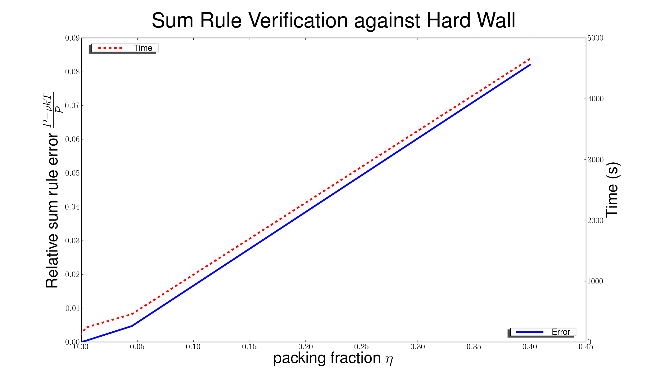
Figure 1: Both accuracy and simulation time are shown for a hard sphere liquid of 0.1nm particles. The domain is divided into cubes which are 0.05nm${}\times{}$0.05nm${}\times{}$.00625nm.

VI.2 Ionic fluids

Calculation of ionic densities near a hard wall also provides a sensitive test for the accuracy of the DFT method. In Gillespie et al. (2005b), it is demonstrated that the BF version of DFT (Eq. 14–15) provides qualitatively incorrect densities, when compared with the RFD functional (Eq. IV.3–35) and high resolution Monte Carlo simulation. We have successfully reproduced the one-dimensional DFT and Monte Carlo results with the 3D code, attesting to the accuracy of our approach. Below, we detail a representative simulation.

For our trial calculation, we examine a salt solution of univalent ions. The cation has radius 0.1nm, the anion 0.2125nm. Each species has a 1M bath concentration. The simulation cell, 2nm$\times$2nm$\times$6nm, is periodic in each direction. A hard, uncharged wall is placed a $z=0$. We discretize the density on a 21$\times$21$\times$161 grid. The results are insensitive to the resolution in the transverse ($x-y$) directions, but very sensitive in the normal ($z$) direction. We verify the homogeneity of the solution across $x-y$ planes to machine precision. In Fig. 2 and Fig. 3, we show the excellent match between 1D and 3D DFT results, with MC results shown for comparison. The mean electrostatic potential is shown in Fig. 4, also with good agreement.

The BF calculations are currently much more efficient than the RFD calculations, needing only 1.5 minutes compared to more than a day to run, since BF scales as $\mathcal{O}(N\log N)$, whereas the RFD method scales as $\mathcal{O}(N^{2})$ and additional iterates are needed to obtain a converged reference density. However, the extra investment of time for RFD computations is necessary because the BF solution is qualitatively incorrect compared to Monte Carlo simulations.

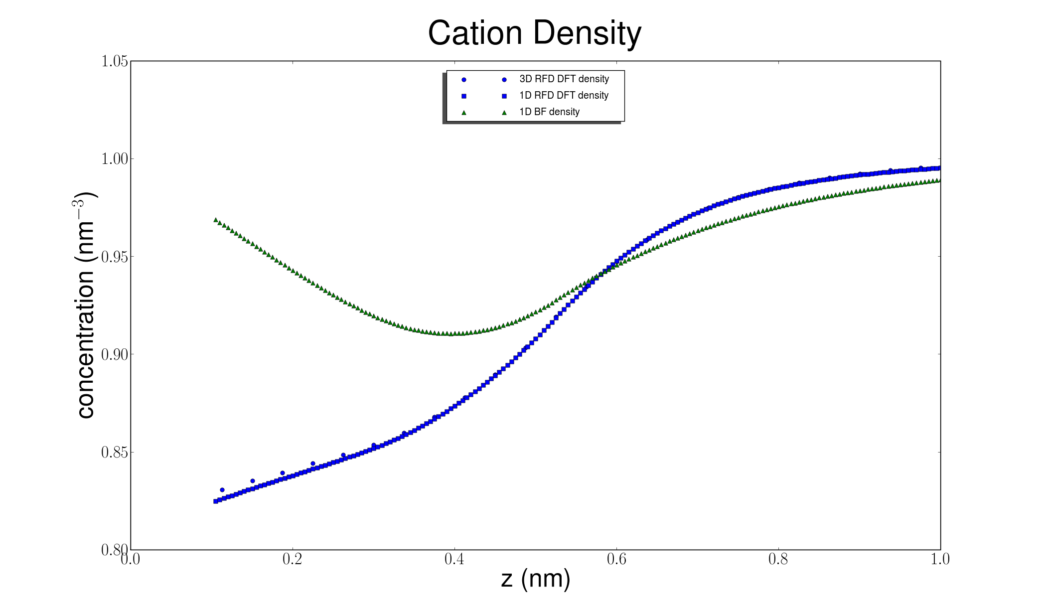
Figure 2: Comparing 1D and 3D DFT cation concentrations to MC simulations. The wall is uncharged, the cation concentration is 1M, and the ions are univalent. The 1D RFD DFT is shown with the blue squares, 3D RFD DFT with blue circles, and MC with green squares.

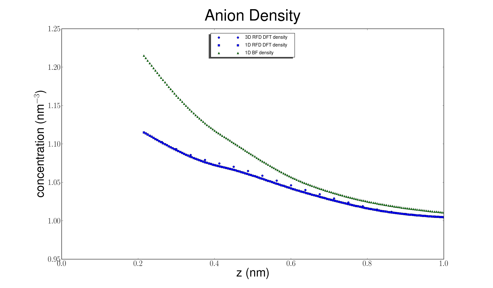
Figure 3: Comparing 1D and 3D DFT anion concentrations to MC simulations. The wall is uncharged, the cation concentration is 1M, and the ions are univalent. The 1D RFD DFT is shown with the blue squares, 3D RFD DFT with blue circles, and MC with green squares.

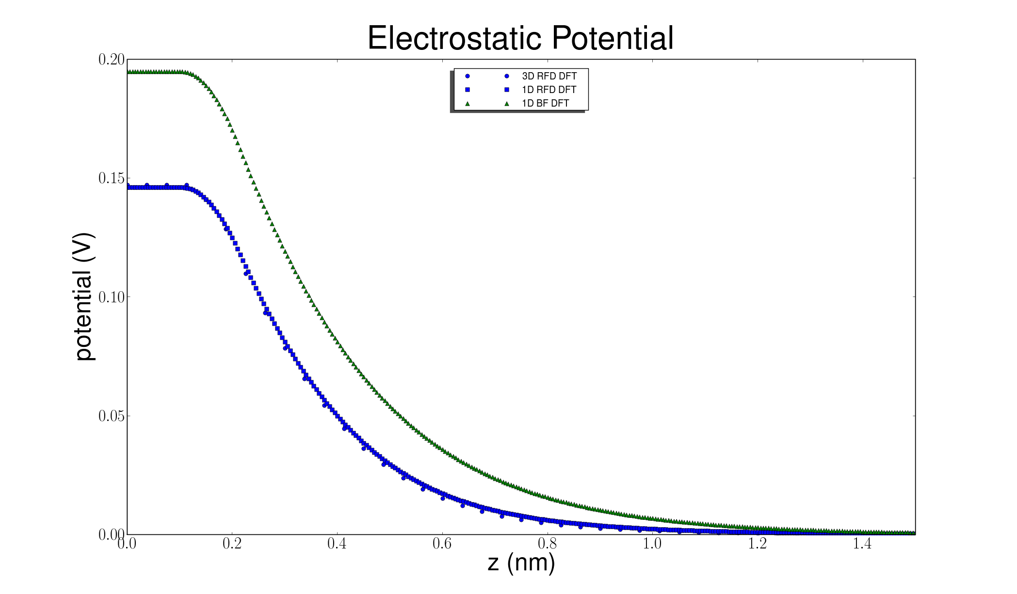
Figure 4: Comparing 1D and 3D DFT mean electrostatic potential to MC simulations. The wall is uncharged, the cation concentration is 1M, and the ions are univalent. The 1D RFD DFT is shown with the blue squares, 3D RFD DFT with blue circles, and MC with green squares.

VII Conclusions and Future Work

We have presented a full numerical strategy for solving the three dimensional equilibrium DFT system. The hard sphere calculation accurately reproduces thermodynamic sum rules, and agrees with prior MC simulation. Moreover, using the improved RFD electrostatic formulation due to Gillespie et al. Gillespie et al. (2002), we can accurately reproduce electrostatic behavior near a hard wall for species of differing radii. Thus, the DFT can now become a powerful tool for full three dimensional chemical simulation, accurately capturing both the energetic and entropic contributions to the solution.

There are also several avenues for improvement of the RFD algorithm and extension of the capabilities of the current code. The dominant cost of this algorithm is the calculation of the reference density used to describe electrostatic screening. The current algorithm is very accurate, but requires $\mathcal{O}(N^{2})$ work. Since the Fourier kernel is smooth and has rapid decay, it should be possible to construct a multiresolution analysis of it, resulting in a fast method for application. Moreover, the many FFTs performed at each Picard step could be replaced by Unequally-Spaced FFTs or wavelet decompositions, which would allow adaptive refinement and increase the size of problems we can efficiently compute. The FFT and Fast Wavelet Transform (FWT) lend themselves readily to a scalable parallel implementations. In fact, it should also be possible to offload these transforms onto a multicore co-processor, such as the Tesla 1060C GPU NVI . This will make large scale simulations of charged hard spheres accessible to working scientists even on a laptop or desktop computer. These algorithmic improvements are the focus of current research.

Appendix A Calculation of the Bath Chemical Potential

Here we describe the formulas for the electrochemical potential in a homogeneous fluid. When the DFT for hard spheres uses a Percus-Yevick equation of state Lebowitz (1964), and the electrostatics is described using MSA Waisman and Lebowitz (1972); Blum (1975). We follow the treatment in Nonner et al. (2000). The bath chemical potential $\mu^{bath}_{i}$ has two components, hard sphere and electrostatic,

$$\mu^{bath}_{i}=\mu^{HS,bath}_{i}+\mu^{ES,bath}_{i}$$ (61)

which are calculated thermodynamically Nonner et al. (2001),

$$\mu^{HS,bath}_{i}=kT\left(-\ln\Delta+\frac{3\xi_{2}\sigma_{i}+3\xi_{1}\sigma_{i}^{2}}{\Delta}+\frac{9\xi_{2}^{2}\sigma_{i}^{2}}{2\Delta^{2}}+\frac{\pi P^{HS}_{bath}\sigma_{i}^{3}}{6kT}\right)$$ (62)

based upon the auxiliary variables, where $\sigma_{i}$ is the ion diameter of species $i$,

$$\xi_{n} = \frac{\pi}{6}\sum_{j}\rho^{bath}_{j}\sigma_{j}^{n}\qquad n\in\{0,\ldots,3\}$$ (63)

$$\Delta = 1-\xi_{3}$$ (64)

and the pressure due to hard sphere interaction in the bath,

$$P_{bath}^{HS}=\frac{6kT}{\pi}\left(\frac{\xi_{0}}{\Delta}+\frac{3\xi_{1}\xi_{2}}{\Delta^{2}}+\frac{3\xi_{2}^{3}}{\Delta^{3}}\right).$$ (65)

The calculation of $\mu_{i}^{HS,bath}$ as given above is straightforward, but $\mu_{i}^{ES,bath}$, on the other hand, is dependent on an implicitly defined parameter $\Gamma$, the MSA inverse screening length,

$$4\Gamma^{2}=\frac{e^{2}}{kT\epsilon}\sum_{j}\rho^{bath}_{j}\left(\frac{z_{j}-\eta\sigma^{2}_{j}}{1+\Gamma\sigma_{j}}\right)^{2}$$ (66)

where $\eta$ represents the effects of nonuniform ionic diameters

$$\eta=\frac{1}{\Omega}\frac{\pi}{2\Delta}\sum_{j}\frac{\rho^{bath}_{j}\sigma_{j}z_{j}}{1+\Gamma\sigma_{j}}$$ (67)

and $\Omega$ is determined by

$$\Omega=1+\frac{\pi}{2\Delta}\sum_{j}\frac{\rho^{bath}_{j}\sigma^{3}_{j}}{1+\Gamma\sigma_{j}}$$ (68)

This implicit relationship is a quartic equation in $\Gamma$, which we solve using Newton’s method. We may then calculate the bath potential

$$\mu^{ES,bath}_{i}=-\frac{e^{2}}{4\pi\epsilon\epsilon_{0}}\left[\frac{\Gamma z^{2}_{i}}{1+\Gamma\sigma_{i}}+\eta\sigma_{i}\left(\frac{2z_{i}-\eta\sigma^{2}_{i}}{1+\Gamma\sigma_{i}}+\frac{\eta\sigma^{2}_{i}}{3}\right)\right].$$ (69)

Appendix B Evaluation of the Fourier Transform of the Weighting Functions

We must be careful to evaluate our analytic transforms at the same $\vec{k}$ values, in the same order, as those computed using the particular implementation of FFT we use. Given a $D$ dimensional grid, the vector $\{k_{d}\}$ which corresponds to the vertex $\{j_{d}\}$ of our Cartesian grid is given by

$$k_{d}=\begin{cases}\frac{2\pi j_{d}}{N_{d}h_{d}}&j_{d}\leq\frac{N_{d}}{2}\\ \frac{-2\pi(N_{d}-j_{d})}{N_{d}h_{d}}&j_{d}>\frac{N_{d}}{2}\end{cases}$$ (70)

where $N_{d}$ is the number of grid points in dimension $d\in\{x,y,z\}$, and $h_{d}$ is the grid spacing $\frac{L_{d}}{N_{d}-1}$.

We begin with the calculation of $\hat{\omega}^{2}_{i}$,

$$\hat{\omega}^{2}_{i} =\int^{2\pi}_{0}d\phi\int^{\pi}_{0}d\theta\sin\theta\int^{\infty}_{0}dr\ r^{2}\delta\left(|r|-R_{i}\right)e^{-\imath\vec{k}\cdot\vec{x}}$$ (71)

$$=\int^{2\pi}_{0}d\phi\int^{\pi}_{0}d\theta\sin\theta R^{2}_{i}e^{-\imath R_{i}\vec{k}\cdot\hat{x}}.$$ (72)

We now choose a rotated coordinate system (the prime system) in which $\vec{k}$ points purely in the $z^{\prime}$ direction, in order to take advantage of the rotational symmetry of the problem. In the new coordinate system,

$$\hat{\omega}^{2}_{i} = \int^{2\pi}_{0}d\phi^{\prime}\int^{\pi}_{0}d\theta^{\prime}\sin\theta^{\prime}R^{2}_{i}e^{-\imath R_{i}k^{\prime}_{z}\cos\theta^{\prime}}$$ (73)

$$= 2\pi R^{2}_{i}\int^{\pi}_{0}d\theta^{\prime}\sin\theta^{\prime}\left(\cos\left(R_{i}k^{\prime}_{z}\cos\theta^{\prime}\right)-\imath\sin\left(R_{i}k^{\prime}_{z}\cos\theta^{\prime}\right)\right)$$ (74)

$$= \frac{4\pi R_{i}\sin\left(R_{i}k^{\prime}_{z}\right)}{k^{\prime}_{z}}$$ (75)

which, in the original coordinate system, is

$$\hat{\omega}^{2}_{i}=\frac{4\pi R_{i}\sin\left(R_{i}|\vec{k}|\right)}{|\vec{k}|}.$$ (76)

From Eq. (8), we also have

$$\hat{\omega}^{0}_{i}=\frac{\sin\left(R_{i}|\vec{k}|\right)}{R_{i}|\vec{k}|}\qquad\hat{\omega}^{1}_{i}=\frac{\sin\left(R_{i}|\vec{k}|\right)}{|\vec{k}|}.$$ (77)

Recognizing that the theta function can be obtained as the integral of a delta function, we have

$$\hat{\omega}^{3}_{i} =\int^{R_{i}}_{0}dr\,\hat{\omega}^{2}_{i}\mid_{R_{i}=r}$$ (78)

$$=\frac{4\pi}{|\vec{k}|}\int^{R_{i}}_{0}dr\ r\sin\left(r|\vec{k}|\right)$$ (79)

$$=\frac{4\pi}{|\vec{k}|^{3}}\left(\sin\left(R_{i}|\vec{k}|\right)-R_{i}|\vec{k}|\cos\left(R_{i}|\vec{k}|\right)\right)$$ (80)

Following a similar procedure as in the $\hat{\omega}^{2}_{i}$ calculation, but keeping track of the vector nature of $\omega^{V1}$ and $\omega^{V2}$,

$$\hat{\omega}^{V2}_{i} = \int^{2\pi}_{0}d\phi^{\prime}\int^{\pi}_{0}d\theta^{\prime}\sin\theta^{\prime}R_{i}^{2}e^{-\imath R_{i}k^{\prime}_{z}\cos\theta\hat{x}}$$ (81)

$$= -2\pi\imath R_{i}\int^{\pi}_{0}d\theta^{\prime}\sin\theta^{\prime}\cos\theta^{\prime}\sin\left(R_{i}k^{\prime}_{z}\cos\theta^{\prime}\right)\hat{k^{\prime}_{z}}$$ (82)

$$= \frac{-4\pi\imath}{|\vec{k}|^{2}}\left(\sin\left(R_{i}|\vec{k}|\right)-R_{i}|\vec{k}|\cos\left(R_{i}|\vec{k}|\right)\right)\hat{k}.$$ (83)

The preceding expressions for $\hat{\omega}^{\alpha}_{i}$ may be evaluated at $|\vec{k}|=0$, but care must be taken when calculating the limit.

$$\underset{|\vec{k}|\rightarrow 0}{\lim}\hat{\omega}^{0}_{i} =\underset{|\vec{k}|\rightarrow 0}{\lim}\frac{\sin\left(R_{i}|\vec{k}|\right)}{R_{i}|\vec{k}|}=1$$

$$\underset{|\vec{k}|\rightarrow 0}{\lim}\hat{\omega}^{1}_{i} =R_{i}$$

$$\underset{|\vec{k}|\rightarrow 0}{\lim}\hat{\omega}^{2}_{i} =4\pi R_{i}^{2}$$

$$\underset{|\vec{k}|\rightarrow 0}{\lim}\hat{\omega}^{3}_{i} =\underset{|\vec{k}|\rightarrow 0}{\lim}\frac{4\pi}{|\vec{k}|^{3}}\left(\left(R_{i}|\vec{k}|-\frac{\left(R_{i}|\vec{k}|\right)^{3}}{6}\right)-R_{i}|\vec{k}|\left(1-\frac{\left(R_{i}|\vec{k}|\right)^{2}}{2}\right)\right)$$

$$=\frac{4}{3}\pi R_{i}^{3}$$

$$\underset{|\vec{k}|\rightarrow 0}{\lim}\hat{\omega}^{V1}_{i} =0$$

$$\underset{|\vec{k}|\rightarrow 0}{\lim}\hat{\omega}^{V2}_{i} =0$$

It should be noted these are the limits one would expect, since in the $|\vec{k}|=0$ case we are simply integrating either a spherical delta or step function over all space, thereby recovering surface area and volume expressions for a sphere.

Appendix C Directional Average Bound

We can bound the directional average of the density over a sphere in terms of the unweighted average, and thus we can bound the ratio

$$\frac{\left|n^{V2}(x)\right|^{2}}{\left|n^{2}(x)\right|^{2}}$$ (84)

in the calculation of $\Phi(n)$ from Eq. III. We let $\nu(\theta,\phi)$ be the unit vector at the surface of the sphere in the $(\theta,\phi)$ direction. Using Fubini’s Theorem and the Cauchy-Schwarz inequality, we have

$$n^{2}_{V2}(x) = \sum_{ij}\int_{S^{2}}\nu(\theta,\phi)\rho_{i}(x+r)d\Omega\cdot\int_{S^{2}}\nu(\theta^{\prime},\phi^{\prime})\rho_{j}(x+r^{\prime})d\Omega^{\prime}$$ (85)

$$= \sum_{ij}\int_{S^{2}\times S^{2}}\nu(\theta,\phi)\cdot\nu(\theta^{\prime},\phi^{\prime})\rho_{i}(x+r)\rho_{j}(x+r^{\prime})d\Omega d\Omega^{\prime}$$ (86)

$$\leq \sum_{ij}\int_{S^{2}\times S^{2}}|\nu(\theta,\phi)\cdot\nu(\theta^{\prime},\phi^{\prime})||\rho_{i}(x+r)\rho_{j}(x+r^{\prime})|d\Omega d\Omega^{\prime}$$ (87)

$$\leq \sum_{ij}\int_{S^{2}\times S^{2}}|\nu(\theta,\phi)||\nu(\theta^{\prime},\phi^{\prime})|\rho_{i}(x+r)\rho_{j}(x+r^{\prime})d\Omega d\Omega^{\prime}$$ (88)

$$\leq \sum_{ij}\int_{S^{2}\times S^{2}}\rho_{i}(x+r)\rho_{j}(x+r^{\prime})d\Omega d\Omega^{\prime}$$ (89)

$$= \sum_{ij}\int_{S^{2}}\rho_{i}(x+r)d\Omega\int_{S^{2}}\rho_{j}(x+r^{\prime})d\Omega^{\prime}$$ (90)

$$= n^{2}_{2}(x)$$ (91)

so that

$$\frac{\left|n^{V2}(x)\right|^{2}}{\left|n^{2}(x)\right|^{2}}\leq 1.$$ (92)

References

- Evans (1979) R. Evans, Adv. Phys. 28, 143 (1979).
- Wu (2006) J. Wu, J. AIChE 52, 1169 (2006).
- Gillespie et al. (2005a) D. Gillespie, L. Xu, Y. Wang, and G. Meissner, J. Phys. Chem. B 109, 15598 (2005a).
- Gillespie (2008) D. Gillespie, Biophys. J. 94, 1169 (2008).
- Roth et al. (2002) R. Roth, R. Evans, A. Lang, and G. Kahl, J. Phys.: Condens. Matter 14, 12063 (2002).
- Yu and Wu (2002a) Y.-X. Yu and J. Wu, J. Chem. Phys. 117, 10156 (2002a).
- Hansen-Goos and Roth (2006) H. Hansen-Goos and R. Roth, J. Phys.: Condens. Matter 18, 8413 (2006).
- Gillespie et al. (2002) D. Gillespie, W. Nonner, and R. S. Eisenberg, J. Phys.: Condens. Matter 14, 12129 (2002).
- Gillespie et al. (2003) D. Gillespie, W. Nonner, and R. S. Eisenberg, Phys. Rev. E 68, 031503 (2003).
- Yu and Wu (2002b) Y.-X. Yu and J. Wu, J. Chem. Phys 116, 7094 (2002b).
- Rosenfeld (1993) Y. Rosenfeld, J. Chem. Phys. 98, 8126 (1993).
- Rosenfeld (1989) Y. Rosenfeld, Phys. Rev. Lett. 63, 980 (1989).
- Evans (1992) R. Evans, Fundamentals of Inhomogeneous Fluids (CRC, 1992), chap. Density functionals in the theory of nonuniform fluids, pp. 85–176.
- (14) URL https://software.sandia.gov/DFTfluids/index.html.
- Gillespie et al. (2005b) D. Gillespie, M. Valiskó, and D. Boda, J. Phys.: Condens. Matter 17, 6609 (2005b).
- Rosenfeld et al. (1997) Y. Rosenfeld, M. Schmidt, H. Löwen, and P. Tarazona, Phys. Rev. E 55, 4245 (1997).
- Blum and Rosenfeld (1991) L. Blum and Y. Rosenfeld, Journal of Statistical Physics 63, 1177 (1991).
- Waisman and Lebowitz (1972) E. Waisman and J. L. Lebowitz, The Journal of Chemical Physics 56, 3086 (1972), URL http://link.aip.org/link/?JCP/56/3086/1.
- Blum (1975) L. Blum, Molecular Physics 30, 1529 (1975).
- (20) URL http://en.wikipedia.org/wiki/Heaviside_step_function.
- Balay et al. (2009) S. Balay, K. Buschelman, V. Eijkhout, W. D. Gropp, D. Kaushik, M. G. Knepley, L. C. McInnes, B. F. Smith, and H. Zhang, Tech. Rep. ANL-95/11 - Revision 3.0.0, Argonne National Laboratory (2009), URL http://www.mcs.anl.gov/petsc/docs.
- Frigo and Johnson (2005) M. Frigo and S. G. Johnson, Proceedings of the IEEE 93, 216 (2005), special issue on “Program Generation, Optimization, and Platform Adaptation”.
- Martin (1988) P. A. Martin, Rev. Mod. Phys. 60, 1075 (1988).
- Goodman and Sokal (1989) J. Goodman and A. D. Sokal, Phys. Rev. D 40, 2035 (1989).
- Frenkel (2004) D. Frenkel, PNAS 101, 17571 (2004).
- (26) URL http://www.nvidia.com/object/product_tesla_c1060_us.html.
- Lebowitz (1964) J. L. Lebowitz, Phys. Rev. 133, A895 (1964).
- Nonner et al. (2000) W. Nonner, L. Catacuzzeno, and B. Eisenberg, Biophys. J. 79, 1976 (2000).
- Nonner et al. (2001) W. Nonner, D. Gillespie, D. Henderson, and R. Eisenberg, J. Phys. Chem. 105, 6427 (2001).